IEEE JOURNAL OF SOLID-STATE CIRCUITS, VOL. 39, NO. 3, MARCH 2004
511
Built-In Current Sensor for
1IDDQ Testing
Josep Rius Vázquez and José Pineda de Gyvez, Member, IEEE
1
Abstract—This paper presents the implementation of a built-in current sensor for DDQ testing. In contrast to conventional built-in current monitors, this implementation has three distinctive features: 1) built-in self-calibration to the process corner in which the circuit under test was fabricated; 2) digital encoding of the quiescent current of the circuit under test for robustness purposes; and 3) enabling versatile testing strategy through the implementation of two advanced DDQ testing algorithms. The monitor has been manufactured in a 0.18CMOS technology and it is based on the principle of disconnecting the device under test from the power supply during the testing phase. The monitor has a resolution of 1 A for a background current less than 100 A or 1% of background currents over 100 A to a total of 1-mA full scale. The sensor operates at a maximum clock speed of 250 MHz. The quiescent current is indirectly determined by counting a number of clock pulses which occur during the time the voltage at the disconnected node drops below a reference voltage value. Basically, at the end of the count period, the counted value is inversely proportional to the quiescent current of the device under test. Then, a DDQ unit processes the counted number and the outcome is compared with a reference number to determine whether a defect exists in the device under test. Accuracy is improved by adjusting the value of the reference number and the frequency of the clock signal depending upon the particular process corner of the circuit under test. The monitor has been verified in a test chip consisting of one “DSP-like” circuit of about 250,000 transistors. Experimental results prove the usefulness of our approach as a quick and effective means for detecting defects.
1
m
1
Index Terms—Current sensors, defects, Deltatesting, sensors.
DDQ , DDQ
I. INTRODUCTION
F
OR ABOUT 25 years, testing of CMOS digital circuits has been recognized as an advantageous methodology to detect defects missed by conventional logic testing. The benefits of this methodology were immediately recognized because of the enhanced observability and sensitivity to defects that do not yet cause a logic fault [1]. Two main test techniques: features can be extracted from today’s 1) differential measurements, e.g., performing some type of comparison between two or more measurements to decide if the circuit is defective or not; and 2) complexity, e.g., it is assumed that the sensing circuit is able to remember the
Manuscript received July 8, 2003; revised October 21, 2003. The work of J. R. Vázquez was supported by the Comisión Interministerial para la Ciencia y Tecnología under Projects TIC2001-2246 and TIC2002-03127, and the Secretaría de Estado de Educación, Universidades, Investigación y Desarrollo in Spain. J. R. Vázquez is with the Departament d’Enginyeria Electrònica, Universitat Politècnica de Catalunya, 08028 Barcelona, Spain, on sabbatical leave with Philips Research Laboratories, 5656 AA Eindhoven, The Netherlands (email:
[email protected]). J. Pineda de Gyvez is with Philips Research Laboratories, 5656 AA Eindhoven, The Netherlands (e-mail:
[email protected]). Digital Object Identifier 10.1109/JSSC.2003.822900
measurements in a previous time or location. As a practical example of such complexity, the test of a high-performance microprocessor was possible by combining multiple techniques such as lowering temperatures, back-biasing, multi- , and testing [2]. These features hold a deep influence on sensors needed to test modern the characterization of deep-submicron ICs. For the interested reader, a review of many current sensors (until 1998) can be found elsewhere [3]. Sensors using a bypass transistor were first presented by Keating and Meyer [4]. They proposed to measure the quiesand cent current by opening a switch connected between the circuit under test (CUT) to observe the decaying voltage node. Since then, this concept has been at the virtual used in both on-chip [5] and off-chip [6] implementations. It is interesting to note that the only published case of an industrial implementation [7] uses an on-chip version of the Keating–Meyer proposal. This probably stems from the fact that built-in sensors have to cope with the impact of process variability [8]. Process variations affect the threshold voltage and thus the leakage current, mainly via the spread in the effective channel length [9]. Variations from two to three orders of magnitude of the leakage current have been reported [8], [10], [11] in real circuits implemented in deep-submicron technologies. This fact causes manufacturer skepticism about the behavior of BICS in a real industrial environment. At the same time, this fact also reveals the great difficulties to satisfy the required features in the design of such sensor. To overcome the limitations of a monolithic implementation, several solutions have been proposed to cope with this problem, namely, solutions that exploit the correlation between and other more accurately known or controlled parameters, e.g.: 1) spatial correlations such as clustering, neighborhood, and transient/quiescent signal analyses [12]–[14]; 2) test pattern correlation including current signatures, current ratios, and [15]–[17]; and 3) time correlation such as speed/current and multiple parameter speed/current correlations [8], [10]. testing is particularly attractive because the differential measurements suppress the impact of the background current. capabilities has been recently An off-chip sensor with implementation is lightly reported [20]. In [21], a algorithm is performed in treated while in [22] the automatic test equipment (ATE). The simplest (and probably the most used) way to make testing is by using the power supply measurement unit of the ATE. Following this approach, it is possible to obtain very accurate measurements with a precision better than a fraction of 1 A. Unfortunately, this approach has an extremely slow test rate, e.g., to obtain accurate measurements of around 100 input vectors can take many minutes of tester time. This fact makes test expensive in an industrial environment. a complete
0018-9200/04$20.00 © 2004 IEEE
512
IEEE JOURNAL OF SOLID-STATE CIRCUITS, VOL. 39, NO. 3, MARCH 2004
TABLE I SUMMARY OF CHARACTERISTICS AND SPECIFICATIONS OF THE PROPOSED BUILT-IN
Thus, to avoid this test time problem, testing is some times reduced to the measurement of the quiescent current with just one input vector, with a limited accuracy. A good summary of actual off-chip solutions is presented in [18]. Further information about off-chip sensors can be found in [6] and [19]. This paper presents the design and implementation of a built testing in a 0.18CMOS techin current monitor for nology. The sensor has a resolution of 1 A for a background current less than 100 A or 1% of background currents over 100 A to a total of 1-mA full scale. The sensor operates at a maximum clock speed of 250 MHz, overcoming in this way the testing. drawbacks of ATE II. BUILT-IN CURRENT SENSOR FOR DELTA-
TESTING
An important feature of our design is that because it is primarily based on a digital solution, it can easily be ported among technology nodes. The main characteristics and specifications of such sensor are shown in Table I and will be described in more detail in the next subsections. A. Properties of the
Monitor
Our scheme uses a version of the Keating–Meyer approach for testing [4]. It includes an on-chip switch connected between the pin and the CUT (a dual implementation would use a switch connected to ground). As this switch is integrated in the circuit, a faster sensor operation is possible because of the reduction of the circuit’s loading capacitance . Our scheme detects defective circuits by analyzing the differences between measurements of current consumption instead of using the absolute value of such measurements. For this reason, it is not sensitive, in a first-order analysis, to the variability of sensor parameters. Nevertheless, the proposed scheme takes into account the process variability by adjusting its range of measurement and its PASS/FAIL limit according to the impact of the manufacturing process on the circuit’s maximum frequency. Important subjects to test the feasibility of the proposed sensor are the sensor resolution and speed as well as the maximum size of the CUT where the sensor is connected, and, as a consequence, the area overhead. Fig. 1 summarizes the sensor’s operation and helps to oversee the parameters involved in such
1I
MONITOR
Fig. 1. Sensor operation.
subjects. Further, Fig. 1 shows two curves corresponding to low and high leakage scenarios. After applying an input pattern to the CUT and after opening the switch, the supply pin voltage decreases until it reaches the reference voltage . The expression associated with this discharge is (1) where , and is the total circuit’s capacitance including decaps. The time that takes the decaying voltage to reach is measured by a counter, C1, as pe. By replacing by , riods of the clock frequency we obtain (2) That is, the number of C1 counts is inversely proportional to and directly proportional to , , and . We use this formula as well as technology data to estimate the sensor resolution and speed. We define the resolution as the minimum amount of current that the sensor can distinguish. For a resolution of 1 A for A, or 1% of full scale (10 A), has to be equal to or greater than 100. As and are defined before testing, the only parameter that is not controlled is the fraction that depends on the technology and on the CUT itself. Notice that because of process variability, fluctuates as well. Thus, for fixed and , and to ensure a 1% accuracy, the sensor has to be connected to a CUT with a value of well above a given threshold to reach the factor required desired resolution. Table II shows the
IEEE JOURNAL OF SOLID-STATE CIRCUITS, VOL. 39, NO. 3, MARCH 2004
Fig. 2. Detailed implementation of
C=I
1
513
monitor showing delta block diagrams for both “max-min” and “successive” implementations.
higher than 1 mA, there are two possibiliconsuming an ties: the first is to keep the same relative resolution at the cost of less absolute resolution. For instance, in a 180-nm circuit transistors and mA, the relative with resolution is 1%, or 100 A of absolute resolution. The second possibility is to partition the CUT, adding one sensor to each partition. This solution preserves both the relative and the absolute resolution. For example, a circuit with transistors and mA needs ten sensors in a 180-nm technology node.
TABLE II FACTORS FOR PRESENT AND FUTURE TECHNOLOGIES
III. CIRCUIT IMPLEMENTATION for present and future technology generations [24]. As can be seen in Table II, about 1 pF of capacitance between and ground is required for each microamp of for 1% resolution. This figure of merit is easily achieved in present and future technologies. The sensor speed is defined as the number of input patterns that can be applied to the CUT in a unit of time. The sensor works at its maximum speed when it works just with the prescribed resolution (that is, when ) at the maximum possible. The corresponding speed expression is (3) For fixed and , the maximum speed is proportional to . The last column of Table II shows the expected maximum speed achievable. The technology, the process corner, and the temperature determine the size of the CUT checked by one sensor. Using a 1% resolution criterion, mA, the off-state current of the transistors and other parameters extracted from the SIA Roadmap [24], it is possible to calculate the circuit size for 180 and 130 nm for FAST, NOMINAL, and SLOW process corners. For the worst case (FAST corner), the sensor is able to manage circuits with about 0.6 Mtransistors (130 nm) or 0.9 Mtransistors (180 nm). For circuits with greater size, thus
The proposed scheme has three blocks: the measurement block (MEAS), the control block (CTRL), and the block (DELTA) which executes two testing algorithms (see Fig. 2). The MEAS block converts a voltage drop proportional to the quiescent current into a digital word that is bits long. It includes a switch to disconnect the device under testing phase. test from the power supply during the The DELTA block captures this word and applies the algorithms to obtain a PASS/FAIL signal. The CTRL block extracts information of the CUT’s actual silicon speed and uses it to define the time base needed by the MEAS block and the threshold level that the DELTA block needs to distinguish between defective and defect-free circuits. built-in current monitor comprises a Essentially, our counter which counts clock pulses during a fixed period to obtain a counted number of clock pulses (MEAS block). The count period has a start determined by the start of the testing cycle which occurs at the instant the switch disconnects the power supply from the device under test. The node connected to the CUT is a “virtual” power supply node (VVDD). The voltage at this virtual node starts decaying due to the quiescent current that discharges the CUT’s capacitance that is intrinsically present at the terminal. The count period may start at the start of the testing cycle, or a predetermined delay time after the start of the testing
514
cycle. The end of the count period is determined through a comparator that detects that the voltage at the input crosses a reference value. Unlike conventional approaches, we determine the quiescent current by counting the number of clock pulses which occur until the voltage at the virtual node drops below a reference voltage value. Basically, at the end of the count period, the count value of the counter is inversely proportional to the CUT’s as shown in (2), if the capacitance of the CUT and the are assumed constant, which is an acceptable assumption in the range of supply voltages in which the test is performed. A post-processing unit (DELTA block) processes the counted number and the outcome is compared with a reference number to determine whether a defect exists in the device under test. To improve the defect detection accuracy, a control circuit (CTRL block) controls the value of the reference number and the frequency of the counter clock signal in dependence on the particular process parameters of the circuit under test. A. MEAS Block The measurement block works as follows: assume that the CUT (which is symbolized in Fig. 2 by the current source and the capacitance ) is in the quiescent state, then the switch is opened and the voltage in the VVDD node starts to decrease due to discharge of . As long as this voltage is greater than a reference, the comparator enables counter C1, which counts the number of clock periods (the time) this voltage takes . When the VVDD voltage reaches the reference to reach voltage, counter C1 stops counting. At this moment, the output of C1 stores a value (coded in bits) which is inversely proportional to . To prevent malfunctioning of the switch or comparator, an overflow signal limits the maximum time that counter C1 is enabled. The switch is basically a pMOS transistor that is connected between the power supply pin (VDD) and the CUT power ring (VVDD). This switch is actually not an integral part of the sensor design because it needs to be tailored specifically for each distinct CUT. If the CUT is in the normal operating mode, the switch is closed and in each transient, a voltage drop across the switch resistance is produced. Obviously, the core’s effective supply voltage reduces, resulting in a loss to of performance. Thus, we need to limit the maximum maintain this loss of performance within acceptable levels. In to 100 mV, our test chip, we have limited the maximum V. which is an acceptable value for a nominal Deciding what is the proper size of the pMOS switch for a is equivalent to knowing what is the given maximum current flowing in the switch. The current specification of the target CUT is 0.59 mA/MHz at 1.8 V. The maximum speed is 100 MHz, consequently, the average current at this frequency is 59 mA. By assuming that at this frequency the current waveform is a triangle, the peak current will be 118 mA. If a mV is acceptable, this means that we maximum need to design a transistor with a channel resistance of 0.848 . An analog comparator is used to compare the decaying . Variations in VVDD voltage and the voltage reference resolution, delay, and offset voltage can be managed because a die-to-die variation in these parameters is not critical as long as it affects each measurement in the same manner. The
IEEE JOURNAL OF SOLID-STATE CIRCUITS, VOL. 39, NO. 3, MARCH 2004
comparator’s unity gain bandwidth is 27.7 MHz with 64-dB gain at dc. This comparator requires a 500-ns stabilization phase for offset compensation and has a minimum safe window of 50 ns for comparison. The comparator uses additional circuitry to compensate offset voltage. The ranges in temperature and supply voltage are 40 C to 85 C and 1.6 to 2 V. In (nominal our 0.18- m test chip, the difference between value is 1.8 V) and is 300 mV, which is small enough to guarantee that the CUT state does not change during the measurement process. B. CTRL Block As is known, the of a defect-free circuit may change by orders of magnitude due to process variations. Therefore, the clock frequency of counter C1 has not only to be very high to curobtain enough precision in the measurement of high rents, but also has to be large to measure the long time counted is small. To handle these requirements, the by C1 when CTRL block is divided into two subblocks (see Fig. 2). The first, which is composed of a ring oscillator, the counter C2 and the blocks Freq. Scaler and Reg. AUX, improves the resolution of measurement by adapting the clock frequency of C1 the to the manufacturing process point in which the chip is fabricated. The proposed scheme takes advantage of the correlaand chip speed [8] to reduce the expected tion between variability that the sensor needs to take into acrange of count. Basically, there is an exponential relationship between speed and leakage. Thus, a measurement of the circuit speed measurement starts, and this inis performed before the formation is used to set the clock frequency of the counter C1 to a proper value. This solution reduces the size of counter C1 to obtain the required precision. The ring oscillator’s frequency is measured in terms of the number of counts that counter C2 reaches in a known period of time. This number of counts is introduced in the Freq. Scaler block, which selects the proper clock frequency for C1. The speed information is also used to set alregister AUX which stores the limit of the maximum lowed for this CUT. The other subblock inside the CTRL block is labeled CONTROL. It supplies the control signals to the counters and registers of the sensor from an external clock (CK) and a Test signal to enable it. C. DELTA Block According to the previous description, we have for each test pattern a word that is bits long, which conveys the measured for this pattern. If test patterns are applied to the CUT, words of bits. the test results are stored in a vector of The DELTA block is a built-in implementation of the technique that digitally processes this information. Two algorithms have been implemented in the sensor: the max-min algorithm and the successive algorithm. The relative benefits of these approaches are analyzed elsewhere [11]. technique [11], There are several approaches to the [23]. The max-min algorithm detects defective circuits by analyzing if the difference between the maximum and the of the CUT is greater than a given threshold. minimum It works as follows. First, the contents of registers Rmax and Rmin are initialized to 00 00 and 11 11, respectively. After
IEEE JOURNAL OF SOLID-STATE CIRCUITS, VOL. 39, NO. 3, MARCH 2004
515
1
Fig. 4. monitor with circuit under test showing additional circuitry I for simulating a large background current and defects.
Fig. 3.
Microphotograph of
1I
monitor.
each measurement, the contents of counter C1 is stored in register R. Then, this value is compared to the content of Rmax, the contents of R registers Rmax and Rmin. If R Rmin, R is stored in Rmin. are stored in Rmax, and if R The difference Rmax Rmin is performed synchronously, and this result is compared to the threshold stored in AUX, thus supplying a PASS/FAIL signal. The second algorithm presented in Fig. 2 is based on the calculation of the difference between successive test patterns (successive). It uses a register R to store the value of C1 in the previous test pattern, a circuit to calculate the absolute value of the difference between the contents of C1 and R, and a digital comparator that compares this difference to a threshold stored in AUX. The output of this comparator is a PASS/FAIL signal. The result of each algorithm is presented at the internal signals pnf_successive and pnf_maxmin. One of them is selected to drive the output pin passnfail. The selection is made by the flip-flop FF_mux, which is loaded during the initialization phase. IV. EXPERIMENTAL RESULTS This section presents results obtained from measuring built-in sensor. Fig. 3 shows a 24 samples of the microphotograph of the monitor (0.09 mm ) along with the DSP-like cor1e (0.8 mm ) used for testing. We did not find any real defects from the test chips received. Also, the background current of the core was around 3 A. Thus, to fully explore the capabilities of the sensor, we artificially introduced defects and elevated the background current as well. Fig. 4 shows is a resistor used to introduce how we tested the sensor. R is the resistor used to vary our artificial defect and R the background current. is a decoupling capacitance needed when the background current is artificially increased . Further, Fig. 4 shows a block diagram of by means of R sensor and the name of the main signals. Signal the test starts the sensor operation, signal test2 opens and closes the switch and signal ck_tester is the external clock signal
is connected to the internal supplied by the ATE. Signal DSP power ring. There is no external load connected to this pin (except eventually an oscilloscope probe). The current source models the DSP quiescent current. A. Speed Measurement and Correlation With Leakage Current Despite the reduced sample size, we observe a dispersion of about 6.2% around the average frequency of 111.8 MHz of the ring oscillator’s frequency . To calculate the corre, a previously calculated value sponding quiescent current, (651 pF) is assumed and then of the internal capacitance used in the equation (4) In our experiments, V, , nF, and is the contents of the R register. Fig. 5(a) and and without and (b) shows the correlation between with extra background current, respectively. In both cases, the contents of counter C1 were obtained by reading register R for a test vector. The reading was made only once, thus, given the value obtained is a single sample. As can be seen, in spite and of the reduced sample size, the correlation between is clearly visible. However, the dependence appears as linear and not exponential, because of the tight process window and the reduced statistical significance of the sample. B. Voltage Drop in the Switch When the DSP is excited with stuck-at vectors, the switch is closed and the effective DSP supply voltage suffers a small reduction. This fact can be seen in the waveforms shown in voltage Fig. 6. This figure shows the reduction in the DSP’s during the first loading of the DSP’s scan chains (the small dip in the waveform labeled scanin). This drop is just before the first measurement is done (first DSP vector). Notice how the voltage drop has a trapezoidal shape. This is because the scan chain is progressively loaded with more and more data, thus activating more and more parts inside the DSP. As a consequence, the DSP has progressively more switching activity and the drop voltage increases. The sudden variation in the voltage drop at the
516
IEEE JOURNAL OF SOLID-STATE CIRCUITS, VOL. 39, NO. 3, MARCH 2004
(a)
Fig. 6.
Voltage at virtual node.
(b) Fig. 5. Correlation of leakage and circuit speed. (a) Leakage and speed correlation of test chips. (b) Leakage and test correlation with emulated background current.
beginning and at the end of the scan activity is due to the DSP’s voltage needs to be taken clock. The perturbation of the into account during testing because this voltage takes some time to reach its quiescent state after the scan activity is stopped. After that the DSP scan stops, a time pause is enforced measurement. In before opening the switch to begin the this case, the voltage is stable and no measurement errors are produced. C. Detecting Defects With the
Sensor
Unfortunately, we did not detect any real defects in any of the 24 IC samples. Thus, it was impossible to test the sensor correctness in the presence of a real defect. Furthermore, the as is demonstrated samples come from a lot with very low by the measurements. Thus, to check the proper sensor behavior, we artificially introduced “defects” in the ICs. The strategy was that was at 0 or at 1 in different to use a DSP output pin between and the vectors, and to connect a resistor R node, thus emulating the presence of a defect. Each time was at 0, there was a small extra current added to . was at 1, a small extra current was subtracted to . If , we emulate the presence of In this way, by changing R . We introduced an a defect drawing different values of extra current of about 0.8 A with R k and then measured the threshold of detection of this “defect.” The test detects four fails [see Fig. 7(a)]. Fig. 7(b) successive test that detects a defect in the ninth shows a max-min DSP vector. To evaluate false detects, we measured the noise threshold vector to vector. The procedure is plus the variations on as follows. We know that the minimum defect current that can be detected is around 0.8 A, and that exactly four detects are
(a)
Fig. 7. Fault detection with the (b) Max-min algorithm.
1I
(b) monitor. (a) Successive algorithm.
flagged by the successive test. Then, to measure the noise threshold we lower the threshold stored in register AUX
IEEE JOURNAL OF SOLID-STATE CIRCUITS, VOL. 39, NO. 3, MARCH 2004
517
V. CONCLUSION
Fig. 8.
Evaluation of the monitor’s sensitivity to false detects.
Defect-free digital ICs of actual and future technologies have an increase in both the absolute value and the variability of their current due to a defect quiescent current. Thus, the extra is a small percentage of the total current. As a consequence, the single PASS/FAIL current threshold approach to distinguish defective circuits is not feasible. Several solutions have been proposed to reduce the absolute value and variability of the current, thus lengthening the usefulness of the testing. All of them propose complex computations to distinguish defective circuits. To be useful and practical, sensors for current testing have to implement one or more of the previous solutions. Off-chip sensors can be more accurate than the on-chip ones, however, they are inherently slower. Since the test speed is an important issue, an on-chip solution is more appropriate. We presented a built-in current sensor in a 0.18- m CMOS for self calibration technology that correlates speed and due to process variations. The sensor implements two test algorithms, has a maximum speed of 2.5 Mvectors/s at max, and a resolution of A of full imum scale (maximum 1 mA). The sensor is robust, fast, and presents a plausible solution for a built-in current sensor in present and future technologies. ACKNOWLEDGMENT The authors would like to thank Dr. Kruseman and Dr. Pelgrom for fruitful discussions. REFERENCES
Fig. 9. I algorithms.
variations vector to vector plus noise measurements of both
until we have more than four detects. Likewise, we raise the contents of register AUX until we have less than four detects. These are the lower and upper bounds of false detects. Fig. 8 shows the combined results. One can see that there is a wide margin between the erroneous and correct detection of the defect for all chips. Notice the logarithmic scale in the y axis. D. Noise Measurements An important issue is the measurement of noise. As node remains “floating” while it is disconnected from the power measurement, the node is susceptible to supply during a collecting noise from the environment. To estimate the measurement noise, we proceeded as follows. Take a defect-free chip (all chips were defect free; we randomly selected chip #3), then threshold (max-min and successive) and exedefine a cute the test 100 times. Count the number of times the passnfail signal is activated, increase the threshold, and repeat. Results thresholds, every test failed are shown in Fig. 9. For low variations vector to vector, and 2) measurement due to 1) noise. By increasing the threshold, the number of fails decreased until reaching zero. Notice the differences between max-min and successive techniques in the decreasing number of fails.
[1] W. Levi, “CMOS is most testable,” in Proc. Int. Test Conf., 1981, pp. 217–220. [2] T. Miyake, T. Yamashita, N. Asari, H. Sekisaka, T. Sakai, K. Matsuura, A. Wakahara, H. Takahashi, T. Hiyama, K. Miyamoto, and K. Mori, “Design methodology of high performance microprocessor using ultra-low threshold voltage CMOS,” in Proc. IEEE Custom Integrated Circuits Conf., 2001, pp. 275–278. [3] A. Ferré, E. Isern, J. Rius, R. Rodríguez, and J. Figueras, “IDDQ testing: state of the art and future trends,” Integration, The VLSI J., no. 26, pp. 167–196, 1998. [4] M. Keating and D. Meyer, “A new approach to dynamic IDD testing,” in Proc. Int. Test Conf., 1987, pp. 316–321. [5] A. Rubio, E. Janssens, H. Cassier, J. Figueras, D. Mateo, P. de Pauw, and J. Segura, “A built-in quiescent current monitor for CMOS VLSI circuits,” in Proc. Eur. Design and Test Conf., 1995, pp. 581–585. [6] K. M. Wallquist, “Achieving IDDQ/ISSQ production testing with QuiCMon,” IEEE Design Test Comput., pp. 62–69, Fall 1995. [7] E. Bohl, T.Th. Lindenkreuz, and M. Meerwen, “On-chip IDDQ testing in the AE11 fail-stop controller,” IEEE Design Test Comput., pp. 57–65, Oct.–Dec. 1998. [8] A. Keshavarzi, K. Roy, and C. F. Hawkins, “Intrinsic leakage in low power deep submicron CMOS ICs,” in Proc. Int. Test Conf., 1997, pp. 146–155. [9] A. Ferre and J. Figueras, “IDDQ characterization in submicron CMOS,” in Proc. Int. Test Conf., 1997, pp. 136–145. [10] A. Keshavarzi, K. Roy, M. Sachdev, C. F. Hawkins, K. Soumyanath, and V. De, “Multiple-parameter CMOS IC testing with increased sensitivity for IDDQ,” in Proc. Int. Test Conf., 2000, pp. 1051–1059. [11] B. Kruseman, R. van Veen, and K. van Kaam, “The future of delta-IDDQ testing,” in Proc. Int. Test Conf., 2001, pp. 101–110. [12] S. Jandhyala, H. Balachandran, and A. P. Jayasumana, “Clustering based techniques for IDDQ testing,” in Proc. Int. Test Conf., 1999, pp. 730–737. [13] W. Daasch, K. Cota, J. McNames, and R. Madge, “Neighbor selection for variance reduction in IDDQ and other parametric data,” in Proc. Int. Test Conf., 2001, pp. 92–100.
518
[14] A. Germida and J. F. Plusquellic, “Detection of CMOS defects under variable processing conditions,” in Proc. 18th VLSI Test Symp., 2000, pp. 195–201. [15] P. Maxwell, P. O’Neill, R. Aitken, R. Dudley, N. Jaarsma, M. Quach, and D. Wiseman, “Current ratios: a self-scaling technique for production IDDQ testing,” in Proc. Int. Test Conf., 1999, pp. 738–746. [16] C. Thibeault, “A novel probabilistic approach for IC diagnosis based on differential quiescent current signatures,” in Proc. 15th VLSI Test Symp., 1997, pp. 80–85. , “Improving delta-IDDQ-based test methods,” in Proc. Int. Test [17] Conf., 2000, pp. 207–216. [18] G. H. Johnson and J. B. Wilstrup, “A general purpose ATE based IDDQ measurement circuit,” in Proc. Int. Test Conf., 1995, pp. 97–105. [19] “A high speed IDDQ monitor circuit,” Int. Patent WO 96/05 553, Aug. 1995. [20] Q-Star Test [Online]. Available: http://www.qstar.be [21] S. Dragic and M. Margala, “A 1.2 V built-in architecture for high frequency on-line IDDQ/delta IDDQ test,” in Proc. IEEE Computer Society Annu. Symp. VLSI 2002, pp. 148–153. [22] P. Lee, A. Chen, and D. Mathew, “A speed-dependent approach for delta IDDQ implementation,” in Proc. 2001 IEEE Int. Symp. Defect and Fault Tolerance in VLSI Systems, pp. 280–286. [23] A. C. Miller, “IDDQ testing in deep submicron integrated circuits,” in Proc. Int. Test Conf., Oct. 1999, pp. 724–729. [24] Semiconductor Industries Association, Int. Technology Roadmap for Semiconductors, 1999.
IEEE JOURNAL OF SOLID-STATE CIRCUITS, VOL. 39, NO. 3, MARCH 2004
Josep Rius Vázquez received the M.S. and Ph.D. degrees in electrical engineering from Universitat Politècnica de Catalunya (UPC), Barcelona, Spain. He is an Associate Professor in the Electronic Engineering Department of UPC, on leave as a Visiting Research Scientist with the Test Group at Philips Research Laboratories, Eindhoven, The Netherlands. His research interests include VLSI design, testing, and power estimation.
José Pineda de Gyvez (M’90) received the Ph.D. degree from the Eindhoven University of Technology, Eindhoven, The Netherlands, in 1991. From 1991 to 1999, he was a Faculty Member in the Department of Electrical Engineering, Texas A&M University, College Station. Since 1999, he has been a Principal Scientist with Philips Research Laboratories, The Netherlands. He is a co-editor of Integrated Circuit Manufacturability: The Art of Process and Design Integration (New York: Wiley/IEEE Press, 1998). His research interests are in the general areas of design for manufacturability and analog signal processing. Dr. Pineda has been an Associate Editor of the IEEE TRANSACTIONS ON CIRCUITS AND SYSTEMS—PART I and an Associate Editor for Technology of the IEEE TRANSACTIONS ON SEMICONDUCTOR MANUFACTURING.