Causal filter selection in microarray data
Gianluca Bontempi Patrick E. Meyer Machine Learning Group, Computer Science Department, Faculty of Sciences ULB, Universit´e Libre de Bruxelles, Brussels, Belgium
Abstract The importance of bringing causality into play when designing feature selection methods is more and more acknowledged in the machine learning community. This paper proposes a filter approach based on information theory which aims to prioritise direct causal relationships in feature selection problems where the ratio between the number of features and the number of samples is high. This approach is based on the notion of interaction which is shown to be informative about the relevance of an input subset as well as its causal relationship with the target. The resulting filter, called mIMR (min-Interaction Max-Relevance), is compared with state-of-the-art approaches. Classification results on 25 real microarray datasets show that the incorporation of causal aspects in the feature assessment is beneficial both for the resulting accuracy and stability. A toy example of causal discovery shows the effectiveness of the filter for identifying direct causal relationships.
1. Introduction Feature selection is the domain of machine learning which studies data-driven methods to select, among a set of input variables, the ones that will lead to the most accurate predictive model (Guyon et al., 2006). Causal inference is the domain of artificial intelligence which aims to uncover causal relationships between variables from observational data (Spirtes et al., 1993). The importance of bringing causality into play when designing feature selecAppearing in Proceedings of the 27 th International Conference on Machine Learning, Haifa, Israel, 2010. Copyright 2010 by the author(s)/owner(s).
[email protected] [email protected]
tion methods has been exhaustively discussed in the seminal paper (Guyon et al., 2007). According to the authors, the benefits of incorporating causal discovery in feature selection include understanding more finely the data structure and making prediction possible under manipulations and some distribution changes. How to incorporate causal discovery issues in filter problems where the ratio between the number of features and the number of samples is high is still an open issue. This is typically relevant in microarray classification tasks where the goal is, for example, to distinguish between tumor classes or predict the effects of medical treatments on the basis of gene expression profiles (Xing et al., 2001). Here, the number of input variables, represented by the number of gene probes, is huge (around several thousands) while the number of samples, represented by the clinical trials, is very limited (a few tens). In this context, the inference of causal relationships between variables plays a major role since more and more biologists and medical doctors expect from data analysis not only accurate prediction models (e.g. for prognostic purposes) but also insights about causes of diseases (e.g. leukemia or diabete) and appropriate therapeutic targets. The role of information-theoretic filters in feature selection has been largely discussed in the machine learning literature. Mutual information and related notions of information theory has been used in several filter algorithms like Ranking (Duch et al., 2003), Markov blanket filter (Koller & Sahami, 1996), Fast Correlation Based Filter (FCBF) (Yu & Liu, 2004), Relevance Filter (Battiti, 1994; Bell & Wang, 2000), Conditional Mutual Information Maximization (CMIM) filter (Fleuret, 2004), Minimum Redundancy Maximum Relevance (mRMR) filter (Peng et al., 2005) and Double Input Symmetrical Relevance (DISR) (Meyer et al., 2008) filter. This paper proposes an information theoretic formulation of the feature selection problem which sheds
Causal filter selection in microarray data
light on the interplay between causality and information maximization. This is done by means of the notion of feature interaction which plays the role of missing link between causal discovery and feature selection. Qualitatively, feature interaction appears when we can model the dependencies between group of attributes only by considering them simultaneously (Freitas, 2001). Consider for instance two input features x1 , x2 and a target class y. It is said that x1 and x2 interact when the direction or magnitude of the relationship between x1 and x2 depends on the value of y. Actually, this can be called a three-way interaction. Higher-order attribute interactions can be defined in a similar way. A nice aspect of the information theoretic formalism is that the interaction between attributes can be formalised on the basis of the notion of mutual information and conditional mutual information (McGill, 1954). At the same time the interaction between variables sheds a light on the possible causal patterns existing between them. The role of interaction in feature selection has already been discussed in the machine learning litterature. Jakulin (Jakulin, 2005) proposes an heuristic based on interaction for selecting attributes within the naive Bayesian classifier. The authors of (Meyer et al., 2008) proposed a filter algorithm which relies on the maximisation of an information theoretic criterion, denoted Double Input Symmetrical Relevance (DISR), which implicitly takes into account the interaction, or complementarity between variables, in the choice of the features. The paper of (Meyer et al., 2008) showed also that the maximisation of the DISR criterion is beneficial to the selection of the Markov blanket in a classification task. It is however known that the Markov blanket is a superset of the set of direct causes of a target y, since it contains beyond direct causes, also the effects (direct descendants) and their parents (also known as spouses). This paper proposes and assesses an original causal filter criterion which aims both to select a feature subset which is maximally informative and to prioritise direct causes. Our approach relies on the following considerations. The first consideration is that the maximization of the information of a subset of variables by forward selection can be shown to be equivalent to a problem of min-Interaction Max-Relevancy (mIMR), where the most informative variables are the one having both high mutual information with the target and high negative interaction (or high complementarity) with the others. The second consideration is that causal discovery differs from conventional feature selection since not all informative or strongly relevant variables are also direct causes. It follows that a causal filter algorithm
should proceed by implementing a mIMR criterion but avoid to consider variables, like effects and spouses, which are not causally relevant. We propose here an approach which consists in restricting the selection to variables which have both positive relevance and negative interaction. Variables with positive interaction (i.e. effects) are penalised and variables with null relevance, even if interacting negatively (i.e. spouses), are discarded. An additional contribution of the paper is that the estimation of three-way interaction terms is sped up by conditioning on the values of the output class. The computational advantage is particularly evident in the Gaussian case, where the computational effort is limited to the computation of few correlation matrices of the inputs. The mIMR filter, was assessed in terms of accuracy on a set of 25 public microarray datasets and in terms of causal inference on a toy dataset. The real data experiment shows that mIMR outperforms most of the existing approaches, supporting the considerations in (Guyon et al., 2007) about the presumed robustness of causal feature selection methods. The causal inference experiment shows that the mIMR strategy leads to a more accurate retrieval of direct causes with respect to other filters.
2. Mutual information and interaction Let us consider three random1 variables x1 , x2 and y where x1 ∈ X1 , x2 ∈ X2 are continuous and y ∈ Y = {y1 , . . . , yC }. The mutual information I(x1 ; x2 ) (Cover & Thomas, 1990) measures the amount of stochastic dependence between x1 and x2 and is also called two-way interaction (Jakulin, 2005). Note that, if x1 and x2 are Gaussian distributed the following relation holds 1 I(x1 ; x2 ) = − log(1 − ρ2 ) 2 where ρ is the Pearson correlation coefficient.
(1)
Let us now consider the target y, too. The conditional mutual information I(x1 ; x2 |y) (Cover & Thomas, 1990) between x1 and x2 once y is given is defined by Z Z Z p(x1 , x2 |y) dx1 dx2 dy. p(x1 , x2 , y) log p(x1 |y)p(x2 |y) The conditional mutual information is null iff x1 and x2 are conditionally independent given y. The change of dependence betwen x1 and x2 due to the knowledge of y is measured by the three-way interaction information defined in (McGill, 1954) as I(x1 ; x2 ; y) = I(x1 ; y) − I(x1 ; y|x2 ). 1
Boldface denotes random variables.
(2)
Causal filter selection in microarray data
This measure quantifies the amount of mutual dependence that cannot be explained by bivariate interactions. When it is different from zero, we say that x1 , x2 and y 3-interact. A non-zero interaction can be either negative, and in this case we say that there is a synergy or complementarity betwen the variables, or positive, and we say that there is redundancy. Because of the symmetry we have I(x1 ; x2 ; y) = I(x1 ; y) − I(x1 ; y|x2 ) = = I(x2 ; y) − I(x2 ; y|x1 ) = I(x1 ; x2 ) − I(x1 ; x2 |y) (3) Since by (3) we derive I(x1 ; y|x2 ) = I(x1 ; y) − I(x1 ; x2 ; y), it follows that by adding I(x2 ; y) to both sides we obtain I((x1 , x2 ); y) = I(x1 ; y) + I(x2 ; y) − I(x1 ; x2 ; y) = = I(x1 ; y) + I(x2 ; y) + I(x1 ; x2 |y) − I(x1 ; x2 ) (4) Note that the above relationships hold also when either x1 or x2 are vectorial random variables.
selects a subset P of v < n variables in v steps by exploring only vi=1 (n − i + 1) configurations. For this reason the forward approach is commonly adopted in filter approaches for classification problems with high dimensionality (Fleuret, 2004; Peng et al., 2005). If v = 1 the optimal set returned by (5) is composed of the most relevant variable, i.e. the one carrying the highest mutual information to y. For v > 1, we need to provide an incremental solution to (5) in order to obtain, given a set of d variables, the d + 1th feature which maximizes the increase of the dependency. We propose an incremental step based on the relation (4). Let XS be the set of the d < v variables selected in the first d steps. In a forward perspective, the optimal variable x∗d+1 ∈ X − XS to be added to the set XS is the one satisfying x∗d+1 = arg
max I((XS ; xk ); y) = h i I(XS ; y)+I(xk ; y)−I(XS ; xk ; y) = = arg max xk ∈X−XS h i I(xk ; y) − I(XS ; xk ; y) (6) = arg max xk ∈X−XS
xk ∈X−XS
2.1. Interaction and optimal feature selection Consider a multi-class classification problem (Duda & Hart, 1976) where x ∈ X ⊂ Rn is the n-variate input and y ∈ Y is the target variable. Let A = {1, . . . , n} be the set of indices of the n inputs. Let us formulate the feature selection problem as the problem of finding the subset X∗ of v variables such that X∗ = arg
max
S⊂A:|S|=v
I(XS ; y)
(5)
In other terms for a given number v of variables the optimal feature set is the one which maximizes the information about the target. Note that this formulation of the feature selection problem, also known as MaxDependency (Peng et al., 2005; Meyer et al., 2008), is classifier-independent. If we want to carry out the maximization (5), both an estimation of I and a search strategy in the space of subsets of X are required. Section 2.3 will discuss the estimation issues. As far as the search is concerned, according to the Cover and Van Campenhout theorem (Devroye et al., 1996), to be assured of finding the optimal feature set of size v, all feature subsets should be assessed. Given the infeasibility of exhaustive approaches for large n, we will limit to consider here only forward selection search approaches. Forward selection starts with an empty set of variables and incrementally updates the solution by adding the variable that is expected to bring the best improvement (according to a given criterion). The hill-climbing search
that is the variable minimizing the interaction I(XS ; xk ; y) with XS and maximizing the relevance I(xk ; y). 2.2. Interaction and causal patterns This section will discuss how the interaction measure sheds light about the potential causal patterns existing between variables. We will limit to consider here patterns of three variables only since, for estimation and computational reasons, we will not consider interactions of degree higher than three. According to the definition (3), a negative interaction between x1 and x2 means that the knowledge of the value y increases the amount of dependence. This situation can occur in two cases: i) the common effect configuration (Figure 1a) (this is also known as the explaining-away effect and ii) the spouse configuration where x1 is the common descendant of y and x2 (Figure 1b). On the contrary a positive interaction between x1 and x2 means that the knowledge of the value y decreases the amount of dependence. This situation can occur in four cases: i) the common cause configuration (Figure 1c) where two dependent effects x1 and x2 become independent once the value of the common cause y is known, ii)-iii) the brotherhood configurations where y is a brother of x1 (x2 ) (Figure 1d) and iv) the causal chain configuration (Figure 1e) where one of the variables (e.g. x1 ) is the cause and the other (e.g. x2 ) is the effect of y. Note that positive interaction can also be considered as synonimous of redundancy.
Causal filter selection in microarray data
It is interesting to remark that if we are interested to identify the set of direct causes of y, the interaction term is able to disambiguate only partially the situation. If on one side, a positive three-way interaction term implies that at least one variable is not a direct cause (Figures 1cde), on the other side negative interaction could be induced by a spouse configuration (Figures 1b). Note that, it is wellknown that, though spouses are not causal, they belong to the Markov blanket set and as such they are strongly relevant for performing an accurate prediction (Tsamardinos & Aliferis, 2003). This is confirmed by Equation (6) which shows that all variables having negative interaction with the selected set Xs (including spouses) bring non-redundant information about the target. How is it then possible to discriminate spouses from direct causes? A possible solution comes from the fact that spouses are independent of the target and as a consequence their mutual information with y is null. A filter algorithm which aims to perform a forward selection of direct causes should therefore implement the minimum Interaction Maximum Relevance strategy (6) but discard variables with a null relevance (even if their interaction is negative). This is the idea that will be implemented in our causal filter mIMR.
2.3. Estimation of the interaction For a given set XS of selected variables, the optimal forward selection step (6) requires the estimation of the interaction term I(XS ; xk ; y) = I(XS ; xk ) − I(XS ; xk |y). The high feature-to-sample ratio nature of the microarray datasets demands a specific approach to the estimation of this quantity. A large amount of litterature on microarray classification converges on the consideration that only simple, constrained and low-variate estimation techniques are robust enough to cope with the noise and the high dimensionality of the problem (Dougherty, 2001). This is confirmed by the success of univariate ranking approaches which are widely used in explorative genomic studies despite of their evident limitations(Saeys et al., 2007). Although the term I(XS ; xk ; y) is multivariate what we propose here is a biased but robust estimator based only on bivariate terms. In order to design such estimator we can take advantage of the following simplifications. Since y is a class and takes value in a finite set of C values {y1 , . . . , yC }, we can write the term I(XS ; xk |y) as follows:
Z Z
log
p(XS , xk |y) p(XS , xk , y)dXS dxk dy = p(XS |y)p(xk |y) =
C X
I(XS ; xk |y = yc )Prob {y = yc }
(7)
c=1
x1
x2
y
x2
x1
y
(a)
(b) x1
y
x1
x2
x2
y
(c) x1
(d) y
x2
(e) Figure 1. a) Common effect pattern, b) spouse pattern c) common cause pattern, d) brotherhood pattern and, e) causal chain pattern .
where Prob {y = yc } is the a-priori probability of the cth class. After this transformation it appears that the estimation of the interaction term requires the estimation of C + 1 terms: the mutual information I(XS ; xk ) and the C conditional mutual information terms I(XS ; xk |y = yc ) , c = 1, . . . , C obtained by controlling the value of the target. In practical terms this boils down to estimate the terms I(XS ; xk |y = yc ) by considering only the portion of the training set for which the target y = yc . Unfortunately each of these terms is highly dimensional because of the term XS . Most of the information theoretic filters proposed in litterature so far proposed several ways to decompose multivariate mutual information terms in a linear combination of low-variate mutual information terms. We recall here the approximations underlying some of the most effective state-of-the-art filter approaches: Max-Relevance (Peng et al., 2005): it uses I(XS ; y) ≈
1 X I(xi ; y) d xi ∈XS
where d is the size of the set XS .
Causal filter selection in microarray data
Conditional Mutual Information Maximisation (CMIM) (Fleuret, 2004): it makes the approximation I(xk ; y|XS ) ≈ min I(xk ; y|xi ) xi ∈XS
Minimum Redundancy Maximum Relevance it approximates (mRMR) (Peng et al., 2005): the total interaction term (i.e. the interaction term when all the components of XS are independent) (Watanabe, 1960): J(XS ; xk ) ≈
1 X I(xi ; xk ) d xi ∈XS
Double Input Symmetrical Relevance (DISR) (Meyer et al., 2008): it adopts the approximation 1 X I((XS , xk ); y) ≈ I((xi , xk ); y) d xi ∈XS
where pc = Prob {y = yc } . The resulting algorithm, called mIMR (minimum Interaction Maximum Relevance), relies on four main ideas: i) avoid to select spouses by restricting the selection to the subset of relevant variables X+ , ii) select incrementally, among the set of variables X+ the ones which minimise the interaction (mI) and maximise the relevancy (MR), ii) simplify the computation of the interaction term by limiting to 3-way interactions and, iv) speed up the three-way interaction computation by conditioning the interaction compution on the value of the target (i.e. restraining the training set to the set of observations with the same output class). Note that in causal terms the mIMR algorithm tends to select features which are both relevant and on average take part to common effect patterns (Figure 1a) with previously selected variables. In order to initialise the mIMR algorithm (10) with a pair of direct causes, we put x∗1 , x∗2 = arg max I((xi , xk ); y). xi ,xk ∈X+
Similarly to what is done in DISR, we adopt a fast approximation of I(XS ; xk ) which consists in replacing the multivariate term by a linear combination of bivariate terms. The two terms of interaction are then approximated as follows 1 X I(xi ; xk ) (8) I(XS ; xk ) ≈ d xi ∈XS 1 X I(XS ; xk |y = yc ) ≈ I(xi ; xk |y = yc ) (9) d xi ∈XS
This means that we restrict to consider only the interaction terms involving both the candidate feature and at most one of the previously selected features.
Table 1 summarizes a set of causal patterns, involving the candidate feature xk ∈ X+ , the selected feature xi ∈ XS and the target y and the related values of relevancy and interaction. Since mIMR maximizes relevance and minimize interaction it appears that such algorithm prioritises the selection of causal variables xk . The only case when interaction is negative but xk is not causal is discarded a-priori since I(xk ; y) = 0 ⇒ xk ∈ / X+ . According to Table 1 it is then reasonable to expect that the mIMR algorithm proceeds by prioritizing the direct causes, penalizing the effects (because of their positive interaction) and neglecting the spouses.
2.4. The min-Interaction Max-Relevancy (mIMR) filter algorithm
Let us now discuss the relation between the mIMR filter and two related state-of-the-art approaches: DISR and mRMR.
Let X+ = {xi ∈ X : I(xi ; y) > 0} the subset of X containing all variables having non null mutual information (i.e. non null relevance) with y. Once the approximations (8) and (9) are done, the forward step (6) can be written as follows
mIMR vs. DISR: the incremental step of the DISR algorithm is X x∗d+1 = arg max I(xk , xi ; y) (11)
x∗d+1 = arg = arg
max
xk ∈X+ −XS
[I(xk ; y) − I(XS ; xk ; y)] =
h i 1 X I(xk ; y) − (I(xi ; xk ; y) = xk ∈X+ −XS d xi ∈XS h = arg max I(xk ; y)+ max
xk ∈X+ −XS
C i 1 X X pc (I(xi ; xk |y = yc ) − I(xi ; xk )) (10) + d c=1 xi ∈XS
xk ∈X−XS
xi ∈XS
In analytical terms, because of (4), if X+ coincides with X the solution of (11) coincides with (10). What makes a difference between mIMR and DISR is that mIMR i) removes variables with no mutual information with the target and ii) decomposes the mIMR criterion into the sum of a relevance and interaction terms. In the Gaussian case (1), the mIMR algorithm requires the computation of the input-output correlation vector and C + 1 input correlation matrices.
Causal filter selection in microarray data Table 1. Causal patterns, relevance and interactions terms. Causal pattern
I(xk ; y)
I(xi ; xk ; y)
xi → y ← xk xi → y → xk xk ← xi → y xk → xi → y xi ← y → xk xk → xi ← y
>0 >0 >0 >0 >0 0
0 >0 >0 >0