Cellular Automata Model on AIS-Based for Variable ... - UPCommons

Journal of Industrial Engineering and Management JIEM, 2015 – 8(3): 674-692 – Online ISSN: 2013-0953 – Print ISSN: 2013-8423 http://dx.doi.org/10.3926/jiem.1347

Cellular Automata Model on AIS-based for Variable Two-way Waterway

Feng Hongxiang1, Bao Xiongguan1*, Zhou Jianghua1, Li Song1, Fang Qionglin2 Faculty of Maritime and Transportation, Ningbo University (China)

1

2

College of Navigation, Jimei University (China)

[email protected], *Corresponding author: [email protected], [email protected], [email protected], [email protected]

Received: December 2014 Accepted: April 2015

Abstract: Purpose: We aim at “heavy traffic direction” and “light traffic direction” in two-way waterway traffic and attempt to promote the transit capacity of two-way waterway system.

Design/methodology/approach: We propose overtaking rules, head-on rules and a cellular automaton model for variable two-way waterway on AIS-based on the basis of NaSch (Nagel-Schreckenberg) model.

Findings: By numerical simulation to the two situations which allow changing lane and prohibit changing lane, we obtain fundamental functions between traffic flux (speed) and density and find that changing lane can promote traffic flux and average speed of two-way waterway system under the premise of no impact to the traffic order, and when waterway ship traffic is dense, flux of waterway system has a visible promotion, and when traffic is sparse, average speed of waterway system adds significantly.

-674-

Journal of Industrial Engineering and Management – http://dx.doi.org/10.3926/jiem.1347

Practical implications: As an implication, we can reach a compromise between traffic efficiency and safety. When no collision risk incurred, the marine administrations should allow involved ships to change lane for overtaking.

Social implications: As a suggestion, Rule 9 and Rule 10 of COLREGs should make some adjustments correspondingly.

Originality/value: The paper presents a method to analyze and promote transit capacity of two-way waterway.

Keywords: cellular automata, vessel traffic flow, variable two-way waterway, changing lane, numerical simulation

1. Introduction In general, two-way waterway is usually composed by inbound lane, outbound lane and separation zone (or separation line). For the safety of navigation, Rules 9 and Rules 10 of Convention on the International Regulations for the Preventing Collisions at sea, 1972 (COLREGs), in fact divides the two-way waterway into two isolated and independent navigable lanes. However ship traffic is always in disequilibrium, and there exist “heavy traffic direction” and “light traffic direction” (Tingting, Qin & Chaojian, 2013) in the waterway. The performance of “traffic disequilibrium” is that, ship traffic is dense in one lane (or some sections of the lane), but sparse in the other (or the others of the lane). As a result, traffic jam incurs in one lane (or some sections of the lane), but in the other lane ship traffic is disengaged. Therefore, we can make full use of the disengaged lane (or some sections of the lane) to promote the capacity of overall waterway. In marine traffic field, the original research of two-way waterway focused on calculating the transit capacity and waterway width by empirical formulas (Fenghua & Xuefeng, 2007; Zhibang & Xin, 2011). During the process of calculation, the two-way waterway is usually treated as two independent waterways, which are hardly to embody the effect of human, machine, environmental and management factors to the waterway capacity. For its virtues which effectively reflect the ship’s response to human and environmental factors in the trajectory (waterway width), ship handing simulator is widely used in waterway research fields shortly after its birth (Inoue, 2000; Kobylinski, 2011; Seong, Jeong & Park, 2012; Yuezong & Hongbo, 2014). However, single-ship handling simulator fails to carry out largescale, real-time and parallel simulation in hardware and software. So empirical formulas and single-ship handling simulator are helpless in the aspect of complex systems problems. Considering the integrity and systematicness of two-way waterway, Tingting et al. (2013) put -675-


forward the concept of “Tidal Reversible Channel”, but the effect of changing lane hasn’t been solved and discussed in their works. For the virtues of discretization in space, time and state, and easy implementation in algorithm on a computer, cellular automata (CA) model has been widely developed and used in traffic flow study. Feng (2013) presented a ship traffic CA model which took marine characteristics into account. In order to simulate ship traffic from the micro view and reveal the effect of lanechanging to waterway transit capacity, the paper establishes a variable two-way waterway CA model on the basis of Feng (2013). The work can be applied to the optimization, organization and management of ship traffic.

2. Cellular Automata Model on AIS-Based for Variable Two-way Waterway The model is formed by an inbound lane and an outbound lane. Each lane is divided into n equal cells. Each cell is either occupied by a ship or empty. The velocity of ship i takes Vi, and Vi  {0,1,2,…, Vmax}, where Vmax is the maximum speed of some type of ships. In the discrete lane, ship i occupies Li cells from i to i + Li – 1 (when inbound) or to i – Li + 1 (when outbound), and Li  {1,2,…, Lmax}, where Lmax is length of the largest ship in waterway.

2.1. Navigational Rules Under normal conditions, ships navigate in their lanes in compliance with “COLREGs 1972” and other related traffic regulations, and no ships shall normally enter a separation zone or cross a separation line. At this time, ships evolve in accordance with the NS ship traffic CA model in Feng (2013).

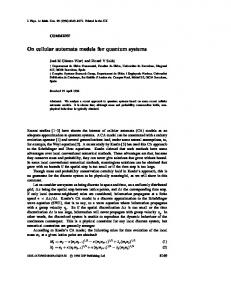
2.2. Overtaking Rules Figure 1 is the sketch-map for overtaking. Suppose at time t, there is ship f1 locating in front of ship i, and (1) Where d1(t) denote the distance from ship i to ship f1, dsafe1 denote the safety distance from ship i to ship f1.

-676-


For the purpose of collision avoidance, ship i has to slow down or stop engine. At this time, if there are enough navigable waters in front of ship f1 and neighbor lane is disengaged, ship i can change to her neighbor lane and overtake ship f1, then goes back to her original lane. Obviously the overtaking action would not impact the safety and traffic order of her neighbor lane, and the transit capacity of overall waterway system promotes.

Figure 1. Sketch-map for overtaking

In the practice of mariner, overtaking vessel should adopt good seamanship. Specifically, overtaking vessel would maintain communication with the overtaken vessel through VHF, make clear her intention of overtaking, and require the overtaken vessel to decelerate or keep speed. Once the overtaken ship agrees to be overtaken, overtaking ship should apply to VTS, and inform her safety measures. With the approval from VTS, overtaking ship may implement her overtaking on the premise of ensuring safety and no impact to the traffic order of her neighbor lane. According to good seamanship, only one ship shall be overtaken each time. Safety conditions to implement overtaking are as follows: (2) (3) (4) (5) Where dsafe2 and dsafe3 respectively denote the safety distances between ship i and her fore ship f2 and aft ship f1 when overtaking is finished; dsafe4 and dsafe5 respectively denote the safety distance between ship i and her fore ship f1_0 and aft ship b1_0 which locate in her neighbor lane; d12 denote the distance between the two nearest ships in front of ship i; d1_0 and db1_0 respectively denote the distances between ship i and her fore ship and aft ship which locate in her neighbor lane; tovertake denote the time to overtake ship i’s fore ship f1; theadon denote the time to head on ship i’s fore ship f1_0 in her neighbor lane.

-677-


2.3. Reverse Navigational Rules for Overtaking In mariner’s practice and in order to reduce the overtaking time, overtaking ship usually accelerates and the overtaken ship decelerates. Therefore, we make the reverse navigational rules for overtaking. Overtaking ship accelerates at each time step, and then navigates at the maximum speed when reaches the maximum. For the overtaken ship, she shall maintain her speed and navigate with caution, so there is no random slowing-down during overtaking. (6) (7) (8) (9) Where pi a n d pf1, respectively, denote random slow probabilities of overtaking ship i and overtaken ship f1.

2.4. Sailing-Back Rules for Overtaking Ship Figure 2 is the schematic diagram of overtaking vessel sailing back to her original traffic lane. When overtaking ship i passes and keeps clear the overtaken ship f1, she shall sail back to her original lane. At this time, the precaution and obligations of overtaking ship and overtaken ship dismiss. Safety conditions to sailing back are as follows: (10) (11)

(12) Where d1_0 and db1_0 respectively denote the distances between ship i and the overtaken ship and the ship in front of the overtaken ship before sailing back.

-678-


Figure 2. Sketch-map for sailing back

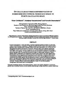
3. Algorithm and Simulation 3.1. Algorithm The algorithm of above-mentioned cellular automata model on AIS-based for variable two-way waterway can describe as in Figure 3.

3.2. Simulation Considering the actual traffic situation, suppose there are 3 types of ships sailing along the two-way waterway, where small-size ship Ls  [30, 89] (m), Vs  [0, 6] (knot), medium-sized ships Lm  [90, 200] (m), Vm  [0, 16] (knot), and large-size ships L1  [201, 300] (m), V1  [0, 12] (knot). The three types of ships mix in the two-way waterway in length of 30 n miles.

-679-


Figure 3. Cellular automata model for variable two-way waterway on AIS-based

3.2.1. Determination of Cell Size and Other Parameters Determination of cell size is usually on the compromise consideration of calculation accuracy and computational complexity by expert judgment (Qu & Meng, 2012). This study takes each cell length of 30 m, and then waterway has 1852 cells in length; and therefore small-size ship Ls  {1,2} (cell) , Vs  {0,1,2,…,6} (cell/t), medium-sized ships Lm  {3,4,5,6} (cell), Vm  {0,1,2,…,16} (cell/t), large-size ships L1  {7,8,9,10} (cell), V1  {0,1,2,…,12} (cell/t).

-680-


3.2.2. Safety Distance According to the discussion in paper (Feng, 2013), the minimum safety distances between ship i and other ships are determined by the following formulas:

(13)

(14)

(15)

(16)

(17)

Where Lf1 and Lf2 respectively denote the lengths of her two nearest ships in front of overtaking ship; Lf1_0 and Lb1_0 respectively denote the lengths of fore ship and aft ship which locate in her neighbor lane; and K = {0,1} denote the running direction of overtaking ship relative to another ship, 0 means inbound and 1 outbound. 3.2.3. Time and Distance Parameters Between Overtaking Ship and Other Ships

(18)

-681-


(19)

(20)

(21)

(22)

(23)

(24)

(25)

-682-


3.2.4. Fundamental Characteristic Parameters of Ship Traffic Flow In order to explicit the kinetic properties of traffic flow; we define two-way channel system and its average density, speed and traffic flux (Rong-Sen, Hui-Li, Ling-jiang & Mu-ren, 2005). (26)

(27) (28) Where Ns, Nm, Nl and s, m, l respectively denote the number and density of small-size ship, medium-size ship and large-size ships, and N is the number of all ships in system. Ship density, speed and flux of one-way direction are determined as follows:

(29)

(30)

(31) Here we introduce ship type mixed proportion coefficient s, m a n d l, where 0  s  1, 0  m  1 and 0  l  1, s + m + l = 1. Then we can get s = s, m = m and l = l, lane traffic density ratio coefficient (32) Where 0 < 1  1 and 0 < 0  1. So density of overall waterway system (33) Where 1 and 0 respectively denote the original density of lane 1 and lane 0. Obviously, if f = 1, original density of the two lanes is equal, otherwise unequal. Because the result of f > 1 is accordant with that of f < 1, we can discuss the situation of f  1 only.

-683-


3.2.5. Ship Generation Model According to on-the-spot observation of ship traffic flow, ship arrival rate obeys Erlang distribution, bow distances between ships follow negative exponential distribution, and ship lengths as well as velocity meet normal distribution.

3.2.6. Simulation Conditions In the next section, we would carry out simulation to explore the relationship between traffic flux (speed) and ship arrival rate. In the simulation, the original status of waterway is unoccupied and random slow probability take 0.25. The input parameter is ship arrival rate, and the simulation of each parameter would repeat for 20 times in order to eliminate the random effects. During each simulation, and for the purpose of equal original simulation conditions, we proceed the situation which allow changing lane first, and at the same time record the ship arrival at entrance, then proceed the situation which prohibit changing lane with former records. Ship arrival rate hereon is the quantity of arrival ships in 1 minute.

4. Simulation and Discussions 4.1 Characteristic of Traffic Flux (Speed) when Inbound and Outbound Traffic is Symmetrical 4.1.1. Spatial-Temporal Spot Diagram of Two-Way Waterway Figures 4 and 5 are respectively inbound spatial-temporal spot diagram of allowing changing and prohibiting changing when inbound and outbound ship arrival rate are both 3. Figures 6 and 7 are respectively outbound spatial-temporal spot diagram of allowing changing and prohibiting changing when inbound and outbound ship arrival rate are both 3. From Figures 4 to 7 we can find that the spatial-temporal spot diagram of allowing changing are more uniform than that of prohibiting changing. During the simulation 16 times changing occur in inbound lane and 35 times in outbound lane, and the trajectories of target lanes are both in order, so the changing actions do not impact waterway traffic order; compared with prohibiting changing, traffic flux and average speed of allow changing promote 4.4 % and 2 % respectively. Because large number of ships in waterway system, increasing quantities of traffic flux and average speed do not seem huge. However for those overtaking ships, economic benefit from the addition of speed and the saving of navigation time and social benefit from the promotion of ship traffic flux are matter-of-course.

-684-


Figure 4. Inbound spatial-temporal spot

Figure 5. Outbound spatial-temporal spot

diagram when allow changing

diagram when prohibit changing



diagram when allow changing

diagram when prohibit changing

-685-


4.1.2. Characteristic of Traffic Flux (Speed) when Inbound and Outbound Traffic is Symmetrical Figures 8 and 9 are respectively the relationship between traffic flux and ship arrival rate when inbound ship arrival rate is symmetrical. In the diagram, changing-lane would promote the traffic flux when inbound or outbound ship arrival rate is big (ship arrival rate is 3, 4, 5 or 6); in the simulation, when ship arrival rate of both lanes are low at the same time (ship arrival rate is 5 or 6), average speed of waterway system would promote 17% at most.

Figure 8. Traffic flux and ship arrival rate as a

Figure 9. Average speed and ship arrival rate as

function when inbound and outbound ship arrival

a function when inbound and outbound ship

rates are symmetrical

arrival rates are symmetrical

4.2 Characteristic of flux (speed) when inbound traffic and outbound traffic is unsymmetrical In the marine practice, the common traffic density in two-way waterway is dynamic and unsymmetrical. So the discussion of unsymmetrical ship density is more significant.

4.2.1. The Relationship Between Traffic Flux and Ship Arrival Rate when Inbound and Outbound Traffic is Unsymmetrical Figures 10 and 11 are respectively the relationship between the flux of waterway system and outbound ship arrival rate at different inbound ship arrival rate when allow changing and prohibit changing. We can find that the flux of waterway system decrease as ship arrival rate increase; when ship traffic flow in waterway is in a free status (ship arrival rate is 4, 5 or 6), traffic flux decreases monotone; and when ship traffic flow is dense, a phenomenon in which ship arrival rate is low and however the traffic flux is low too, occurs in some areas of the -686-


relational diagraphs. The phenomenon is caused by low-speed ship. When there are a large amount of low-speed ships locating in waterway, or when two or more low-speed ships sail one after the other, it’s hard for fast-speed ships to overtake.

Figure 10. Traffic flux of waterway system and

Figure 11. Traffic flux of waterway system

outbound ship arrival rate as a function at variable

and outbound ship arrival rate as a

inbound ship arrival rate (when allow changing)

function at variable inbound ship arrival rate (when prohibit changing)

4.2.2. Compare of Unsymmetrical Inbound and Outbound Traffic when Allow Changing and Prohibit Changing Figures 12 to 17 are respectively the relationship between traffic flux and outbound ship arrival rate when inbound ship arrival rate is determined. In the diagram, changing-lane would promote the traffic flux significantly when inbound or outbound ship arrival rate is both low (ship arrival rate is 1 or 2); what’s more, the bigger inbound and outbound lanes differ, the more ship flux promotes. In the simulation, when ship arrival rate of one lane is 1 and the other is 6, ship traffic of waterway system would promote 11.4% at most.

-687-


Figure 12. Traffic flux of waterway system and


ship arrival rate as a function

and ship arrival rate as a function

(inbound ship arrival rate = 1)














-688-


4.2.3. The Relationship Between Traffic Flux and Ship Arrival Rate when Inbound and Outbound Traffic is Unsymmetrical Figures 18 and 19 are respectively the relationship between traffic flux and outbound ship arrival rate at different inbound ship arrival rate. In the diagram, average speed of waterway system increase as ship arrival rate increases; when ship traffic in waterway is dense (ship arrival rate is 1, 2 or 3), average speed increases monotone; and when ship traffic is in a free status (ship arrival rate is 4, 5 or 6), the regularity of average speed and ship arrival rate is unfirm and irregular in the diagram; explanation to the phenomenon is that the interaction of ships is weak when waterway traffic is in a free status.

Figure 18. Average speed of waterway system


and outbound ship arrival rate as a function at

and outbound ship arrival rate as a function at

variable inbound ship arrival rate (when allow

variable inbound ship arrival rate (when

changing)

prohibit changing)

4.2.4. Compare of Unsymmetrical Inbound and Outbound Average Speed when Low Changing and Prohibit Changing Figures 20 to 25 are respectively the relationship between average speed and outbound ship arrival rate when inbound ship arrival rate is determined. In the diagram, changing-lane would promote the average speed significantly when inbound or outbound ship arrival rate is big (ship arrival rate is 3, 4, 5 or 6); in the simulation, when ship arrival rates of both lanes are low at the same time (ship arrival rate is 5 or 6), average speed of waterway system would promote 17% at most.

-689-




















-690-


5. Conclusions This paper has proposed a cellular automaton model for variable two-way waterway on AIS-based. By numerical simulation to the two situations which allow changing lane and prohibit changing lane, fundamental functions between traffic flux (speed) and density are obtained. That is, the flux of waterway system decreases and the average speed increases as ship arrival rate increases. We so find that changing lane can promote traffic flux and average speed of two-way waterway system under the premise of no impact to the traffic order. When waterway ship traffic is dense, flux of waterway system has a visible promotion, and when traffic is sparse, average speed of waterway system adds significantly. As an implication, we can reach a compromise between traffic efficiency and safety. When no collision risk incurred, the marine administrations should allow involved ships to change lane for overtaking; and as a suggestion, Rule 9 and Rule 10 of COLREGs should make some adjustments correspondingly.

Acknowledgment This work is supported by the National Natural Science Foundation of China (51408322), Zhejiang Provincial Natural Science Foundation of China (LY13A020006), Ningbo natural science funds (Project No.: 2013A610282) and Talent Project of Ningbo University (012-F01273144702).

References Feng, H. (2013). Cellular Automata Ship Traffic Flow Model Considering Integrated Bridge System. International Journal of u- and e- Service, Science and Technology, 6(6): 111-120. http://dx.doi.org/10.14257/ijunesst.2013.6.6.12

Fenghua, L., & Xuefeng, C. (2007). Inquiry on Design Width of Sea Port Channel. Port Engineering Technology, 6. Inoue, K. (2000). Evaluation method of ship-handling difficulty for navigation in restricted and congested waterways. Journal of Navigation, 53(01), 167-180. http://dx.doi.org/10.1017/S0373463399008541

Kobylinski, L. (2011). Capabilities of Ship Handling Simulators to Simulate Shallow Water, Bank and Canal Effects. TransNav-International Journal on Marine Navigation and Safety of Sea Transportation, 5(2), 247-252.

http://dx.doi.org/10.1201/b11343-20

-691-


Qu, X., & Meng, Q. (2012). Development and applications of a simulation model for vessels in t h e S i n g a p o r e S t r a i t s . Expert Systems with Applications, 39(9): 8430-8438. http://dx.doi.org/10.1016/j.eswa.2012.01.176

Rong-Sen, Z., Hui-Li, T., Lingjiang, K., & Mu-ren, L. (2005). The traffic flow of two-lane system with vehicle mixing. Acta Physica Sinica, 54(10), 4614-4620. Seong, Y.C., Jeong, J.S., & Park, G.-K. (2012). The relation with width of fairway and marine traffic flow. TransNav‐International Journal of Marine Navigation and Safety of Sea Transportation, 6(3), 317-321.

http://dx.doi.org/10.1201/b11347-31

Tingting, C., Qin, L., & Chaojian, S. (2013). Scheme Research and Feasibility Analysis of "Tidal Reversible Channel". Navigation of China, 36(2), 55-60. Yuezong, W., & Hongbo, S. (2014). Simulation of Traffic in Two-Way Navigable Channels. Navigation of China, 37(1), 103-107, 130. Zhibang, Z., & Xin, L. (2011). Calculation Method of Channel Navigable Capacity. Port Engineering Technology, 48(6), 15-18.

Journal of Industrial Engineering and Management, 2015 (www.jiem.org)

Article's contents are provided on a Attribution-Non Commercial 3.0 Creative commons license. Readers are allowed to copy, distribute and communicate article's contents, provided the author's and Journal of Industrial Engineering and Management's names are included. It must not be used for commercial purposes. To see the complete license contents, please visit http://creativecommons.org/licenses/by-nc/3.0/.

-692-

Cellular Automata Model on AIS-Based for Variable ... - UPCommons

Cellular Automata Model on AIS-Based for Variable ... - UPCommons

Suggest Documents

Cellular Automata Based Model for Pedestrian Dynamics

A Model Based on Cellular Learning Automata for ...

On cellular automata models for quantum systems

Design of hierarchical cellular automata for on

Cellular Automata

Cellular Automata for Structural Optimization on

ON CELLULAR AUTOMATA REPRESENTATION OF

Cellular Automata

A Survey on Cellular Automata

Cellular Automata

A Survey on Cellular Automata

Stochastic cellular automata model of neural networks

Calibrating a Parallel Geographic Cellular Automata Model

Geographic Spatiotemporal Dynamic Model using Cellular Automata ...

Cellular automata model of magnetospheric-ionospheric coupling

cellular automata model of cardiac pacemaker

Stochastic cellular automata model of cell migration

k-neighborhood for Cellular Automata

Implementing Cellular Automata for Dynamically

Using Cellular Automata on a Graph to Model the

A traffic model based on fuzzy cellular automata - Semantic Scholar

a 2d flood inundation model based on cellular automata approach

A Logistic Based Cellular Automata Model for ... - Springer Link

A Cellular Automata Model for Wireless Sensor ... - Semantic Scholar