JOURNAl_OF
ELSEVIER
Journal of Wind Engineering and Industrial Aerodynamics 67&68 (1997) 387-401
~ ( ~ i ~
Cellular convection embedded in the convective planetary boundary layer surface layer D a v i d S. D e C r o i x , Y u h - L a n g Lin*, D a v i d G. S c h o w a l t e r Department of Marine, Earth and Atmospheric Sciences', North Carolina State UniversiO', Raleigh, NC 27695-8208, USA
Abstract Cellular convection was first studied in the laboratory by Benard [Ann. Chim. Phys. 23 (1901) 62-144] and Rayleigh [Phil. Mag. Ser. 6 (1916) 529 546] investigated these motions from a theoretical perspective. He defined a dimensionless number, now called the Rayleigh number, which is the ratio of convective transport to molecular transport, and found that if a certain critical value is exceeded, cellular convection occurs. Mesoscale cellular convection (MCC) is a common occurrence in the planetary boundary layer. Agee [Dyn. Atmos. Oceans 10 (1987) 317 341] discussed the similarities and differences of MCC and classical Rayleigh-Benard convection. A similar cellular pattern can be seen in the convective boundary layer (CBL) surface layer. It is known that in the CBL, air near the surface converges into thermals producing updrafts. This produces a 'spoke' type pattern similar to the mesoscale cellular or Rayleigh Benard convection. This paper will focus on applying Rayleigh-Benard convection criteria, using a linearized perturbation method, to the CBL surface layer produced by Large Eddy Simulation (LES). We will investigate the length scales of turbulence in the CBL surface layer and compare them to those predicted from linear theory. Similarities and differences will be discussed between the LES produced surface layer and classical Rayleigh-Benard convection theory.
Keywords: Rayleigh-Benard convection; Cellular convection; Large eddy simulation; Planetary boundary layer
1. Introduction Cellular convection was first studied in the laboratory by Benard [1]. He used a very thin layer of fluid, about 1 mm deep, which was heated from below at a constant uniform temperature. He noticed that a number of convective hexagonal cells appeared. These convective cells, shown in Fig. 1, were produced by downward motion
* Corresponding author. E-mail: yl
[email protected]. 0167-6105/97/$17.00 5) 1997 Published by Elsevier Science B.V. All rights reserved. PII S01 6 7 - 6 1 05 ( 9 7 ) 0 0 0 8 8 - 3
388
D.S. DeCroix et al./J. Wind Eng. Ind. Aerodyn. 67&68 (1997)387-401
Fig. 1. Benard cells in spermaceti. From Ref. [17] with permission from Dover.
in the cell center and upward motion on the edges shared with adjacent cells. Lord Rayleigh [2] investigated these motions from a theoretical perspective. He defined a dimensionless number, now called the Rayleigh number, which is the ratio of convective transport and molecular transport. He found that if a certain critical value is exceeded, cellular convection occurs. Classical Rayleigh-Benard (RB) convection was originally thought of as an interesting laboratory phenomenon, but of little meteorological interest. In the 1960's, however, satellites provided meteorologists with their first look at cellular convection in the atmosphere, which often occurs during cold air outbreaks off the eastern coast of North America. In Fig. 2, one sees mesoscale cellular convection (MCC) cells similar to the hexagonal cells Benard discovered in the laboratory. These convection cells may be classified as open or closed. In open (closed) cellular convection, downward motion occurs in the center (edges) of the cell and upward motion on the cell edges (center). Clouds often form in the updraft regions, and in open cellular convection these clouds form hexagonal rings. As discussed by Agee [3] and Stull [4], there are some discrepancies between MCC and RB convection, cell aspect ratio for instance, but the physical mechanism responsible for M C C and RB convection is the same. A similar cellular pattern can be seen in the convective boundary layer (CBL) surface layer. It is well known that in the CBL, air near the surface converges into thermals producing updrafts. In Fig. 5, one sees a 'spoke' type pattern, which was also observed in Schmidt and Schumann's [5] LES results. This pattern is similar to the mesoscale cellular and Rayleigh Benard convection. The CBL in Fig. 5 was modeled
D.S. D e C r o i x et a l . / J .
Wind Eng. Ind. Aerodyn.
I I'
~
£P+
+, •
r?
+
,+~
~,
( ~ ,+;+
~++
~ - ' + ,,~ +,
: +s
'
•
,, .,+ ~+..t:l+, [,j,l l [ ~ , ' ~ +
+..,,¢"~#~+-4 ".t+-+.~ q[ . , ~ .,,t
, .'.~,4~
~.1
~£'.
-
"
,
,'
+ '
+
)+.
. w ~ ;~. .,- :+
"+. . . . .
*~
67&68 (1997) 387-401
389
+
...,
•
+,
....
~ , .
+,++.+++ +
.++.... . +
.
++ ~:
. + ,+++...
"+"
'.~,
"
Fig. 2. Hexagonal cells north of Cuba. From Ref. [3].
using a large eddy simulation (LES) model developed by Proctor [6,7] and North Carolina State University [8]. This paper will focus on applying Rayleigh Benard convection criteria, using a linearized perturbation method, to the CBL surface layer produced by large eddy simulations. Similarities and differences between the LES produced surface layer and classical Rayleigh-Benard convection theory will be discussed. However, there is an inherent difficulty comparing scales of a laminar transition instability to scales in a fully developed turbulent boundary layer. But, as shown by Brown and Roshko [-9], large scale turbulent structures can sometimes be attributed to laminar flow instabilities. We will also investigate the turbulence length scales and structures within the surface layer, and attempt to determine whether the dominant length scales are related to the linear flow instability. We are interested in finding and understanding the length scales in the surface layer, and the planetary boundary layer (PBL), so we can determine what scales interact with aircraft wake vortices. The long term goal of this research, as discussed by Hinton [10], is to quantify the PBL interactions with wake vortices in order to understand and better predict the transport and decay of the vortex.
2. T h e o r e t i c a l
model
Emanuel [-11] performed a linear stability analysis of the Boussinesq form of the Navier Stokes equations. He derived a single equation for the perturbation vertical velocity for the flow between two parallel plates and solved it using a normal mode
390
D.S. DeCroix et al./J. Wind Eng. Ind. Aerodyn. 67&68 (1997) 387 401
Table 1 Critical Rayleigh numbers and horizontal wave numbers for flow between parallel plates Type of boundary
Rac
kc
Both free-slip One no-slip, one free-slip Both no-slip
657.5 1100.7 1707.8
2.22 2.68 3.12
approach. This solution was used to determine the critical stability condition for the fluid system. As a result of the nondimensionalization, the Prandtl number cr and the Rayleigh number Ra were defined as a -=
v
K
,
Ra ~-
gflFH 4
VK
,
(1)
where v is the kinematic viscosity, ~c the thermal conductivity, ,q the coefficient of thermal expansion, F the vertical temperature gradient, and H the fluid layer depth. Emanuel solved the critical flow condition for three vertical (parallel plate) boundary conditions: (1) both upper and lower boundaries are rigid free-slip, (2) the lower boundary is rigid no-slip and the upper is rigid free-slip, and (3) both upper and lower are rigid, no-slip boundaries. Table 1 summarizes these conditions and their corresponding critical Rayleigh and wave numbers. When the Rayleigh number is exceeded, flow instability exists between the two parallel plates. In this paper we will apply the critical Rayleigh and wave number condition for the second boundary condition type, one no-slip, one free-slip rigid boundaries, to flow in the convective boundary layer surface layer generated by large eddy simulation. The supposition is that the CBL surface layer could be thought of as being restricted in the vertical due to the presence of the ground and the CBL mixed layer, which has no potential temperature gradient, and that the cellular pattern seen is due to this mechanism. This upper boundary condition is not strictly valid for the surface layer flow since the upper boundary is not a rigid free-slip boundary, but a limit to the superadiabatic region.
3. The LES model
The LES model used for the simulations is the TASS model developed by Proctor [6,7]. The model was originally developed for the study of thunderstorms and microbursts, but only required a change in boundary conditions for the simulation of the planetary boundary layer [8]. The equations solved are the three dimensional, fully compressible, non-hydrostatic Navier-Stokes equations. A modified
D.S. DeCroix et al./J. Wind Eng. Ind. Aerodyn. 67&68 (1997) 387-401
391
Smagorinsky first order closure is used in which the eddy viscosity is a function of stability through the local flux Richardson number. Equations for water substances, cloud water, cloud ice, snow, hail and graupel, are present in the model, but were not used in these simulations. These equations were solved on an Arakawa C type mesh [12]. Periodic boundary conditions have been used in the horizontal directions, while a sponge layer with three grid intervals has been added on the top of the physical domain. At the top boundary, there exists neither heat nor mass transfer. The lower boundary represents a solid ground plane and employs a no-slip condition. In these simulations, the heat transfer at the surface is computed from the specified ground surface temperature, given as a constant, and the LES computed air temperature at the first grid level above the ground. The reported values of heat flux are the ensemble average of the individual grid point fluxes.
4. Discussion of results The LES model was run on a domain size of 4 km in the N-S and E-W directions and 2 km in the vertical. The grid resolution used was 50 m laterally, with the vertical resolution varied from 10 m near the surface to 50 m at the domain top enabling higher resolution of the surface layer. The model was initialized with a vertical profile or sounding of the environmental pressure, temperature, dew point, u and v vector wind components representative of a dry convective boundary layer. It is not an observed sounding, but rather an idealized sounding for numerical experiments. A specified temperature within the lowest level in the model was used to compute a surface heat flux. In order to initiate the convection, a uniform random temperature perturbation of _+ 1 K (maximum) was applied to the lowest three vertical levels in the domain. The model was run for 2 h of simulation time to develop fully the convective boundary layer. To obtain ensemble averages for the properties in the boundary layer, denoted by ), the variables were averaged in space and time. The variables were averaged at each vertical level in the domain, and then each of those averaged over a time period. After two hours of simulation (spin-up time), the data were output at 2 min intervals for 40 min, producing 20 time-averaging periods. For example, {u'u') was calculated at each vertical level in the model domain by first computing the variance at each grid point in the domain, then horizontally averaging them at each vertical level, and finally averaging each of those horizontal averages over the 20 output times. Three simulations were performed with progressively lower surface temperatures, in order to create supercritical and subcritical Rayleigh number conditions. These surface temperatures used were 287, 285, and 283.75 K, which produced surface heat fluxes of 237, 61, and 18 W/m 2 and are denoted as the high, medium, and low heat flux cases, respectively. In each case, the mean wind was constant with height and less than 1 m/s to diminish any shear instabilities that could be present due to the environment.
392
D.S, DeCroix et al./J. Wind Eng. Ind. Aerodyn. 67&68 (1997) 387 401 25OO
2000
1SO0
J: .p
1000-
t
500-
o 2e3
~
; 284
-,
-
28S
17.6 W / n ~ 2
I
i
J
i
i
¢
4
i
286
2117
2ee
2eg
2go
291
292
Potential Temperature (OK)
Fig. 3. Ensemble averaged potential temperature profile from LES.
4.1. Some properties of the convective boundary layer Fig. 3 shows the potential temperature profiles of each of the three cases. In each profile, the potential temperature is superadiabatic near the surface, nearly constant within the mixed layer, and has an inversion capping the PBL. The surface layer features of the convective boundary layer constitute a mechanism similar to the laboratory Rayleigh-Benard convection. In the laboratory setup, the lower plate is held at a constant temperature which is greater than the upper plate. In the CBL surface layer, the lower surface is also maintained at a constant temperature greater than the mixed layer. This is analogous to the theoretical results for 'one fixed boundary, one free boundary'. Figs. 4 and 5 show the horizontal structure of the vertical velocity and potential temperature. Notice the cellular-type appearance of these contours. These cellular patterns, typical of convective surface layers in the PBL, were the motivation of this paper's research.
4.2. Rayleigh number calculation A Rayleigh number, defined in Eq. (1), was calculated from the fields produced in the LES. For this calculation, the turbulent eddy viscosity, ve, and conductivity, Ke, must be used since the flow is turbulent. From the definition of the eddy viscosity,
P
ve ~zz
~u'w'),
(2)
D.S. DeCroix et al./J. Wind Eng. lnd. Aerodyn. 67&68 (1997) 387-401
, i~e
TASS V e r s i o n 6.19 W at Z 60.2 meters = 122, 0.2 run03
21.0. ~
Fc:i)'"
'
-
393
graph
; -.J :~ ~ °
04 A
00 >-
0.4 -0.8 1.2 -1 6 -2.0 I
195
20.25
21 .8
21 . 7 5 22 g X :KM)
23.25
240
Fig. 4. Vertical velocity c o n t o u r s at 60 m height for the high heat flux case.
TASS V e r s i o n 6.1g Temperature (K) a! Z 6 ~ . 2 meter-s Time = 122, 0.2 runO3.grapln
2~ 1,6 1,2 0.8 04 ~2 >-
0.0 -0
4
-018 -1 I2 1,6 - 2 i0 19.5
20.25
21.0
21 . 7 5 22.5 X (KM)
23.25
24.0
Fig. 5. Potential t e m p e r a t u r e c o n t o u r s at 60 m height for the high heat flux case.
thus for LES,
(3)
394
D.S. DeCroix et aL/J. Wind Eng. Ind. derodyn. 67&68 (1997) 387 401 300
250
200
i
I 2Z'22:
150
100
50
0
I
*
l
l
l
I
10
20
30
40
50
60
v, (m'/s) Fig. 6. Vertical profile of the turbulent eddy viscosity computed from LES.
It should be noted that Eq. (3) is valid only for a non-zero mean wind. For the case of free convection, one could use the eddy viscosity computed within the LES closure model. Using a turbulent Prandtl number (Prt = Ve/~Ce)of 0.89, justified for convective conditions by Businger et al. [13], the Rayleigh number for turbulent flow simulated in LES may be written as Ra -
0.8 9 g fi F H 4 2
(4)
Ye
What is critical in this definition is how one determines the value of ve and H, as they have a very large impact on the computed Rayleigh number. For the CBLs simulated in the LES, Fig. 6 shows the vertical profile of the turbulent eddy viscosity in the surface layer for each heat flux case. There is a large vertical variation in vo and variation for the different cases. A nominal value of 12, 8, and 6 m2/s was chosen for the high, medium and low heat flux cases, respectively. These compare reasonably well with Krishnamurti [14] who reported a value of 30 m2/s for the entire PBL. Krishnamurti's value of Ve was based on Clarke's [15] measurements. Clarke vertically integrated the ageostrophic wind profile to determine the stress, r, as a function of height. Knowing the stress and the velocity gradient with height, he computed the eddy viscosity, in a similar manner as described above. Given the uncertainties in the measured wind, and the assumptions inherent in numerical modeling, the LES and experimentally derived values of t'e are quite comparable. For the region of flow being considered, the surface layer of a convective planetary boundary layer, one must carefully choose values for F and H in Eq. (4). Since we are
395
D.S. DeCroix et al./J. Wind Eng. Ind. Aerodyn. 67&68 (1997) 387 401
interested in cellular convection within the surface layer, F corresponds to the temperature lapse between the surface and the mixed layer, and H to the depth of the surface layer. In order to calculate the potential temperature, 00, at the surface roughness height, Zo, M o n i n - O b u k h o v similarity theory was used. At each vertical level in the model domain, an average u velocity was computed. Using the average u velocity at the first model level, Ua the friction velocity, u,, was computed from: (5)
kua u, = ln(z,/zo) - OM(G/L)"
Using the fact that the surface heat flux is known, 0, may be computed from: (6)
(w'O'> = u , O , .
For stability functions, we use the following for a convective boundary layer (z/L < 0) [ 16]
(,2
On(z/L) = 2 in
+ In - -
- 2 arctan (x) + rr/2,
(7)
O,(z/L)=21n(12x~2),
(8)
x = (1 - 15z/L) 1/4 .
(9)
where
Since the Obukhov length, L, is computed in the LES model at each time step, and with 0. known, 0o, the temperature at Zo, can be computed from: kfOa --
0°}
(10)
0. = Prt[ln (Za/ZO) -- OH(G/L) + O.(zo/L)} ' where Prt = 0.89, the surface turbulent Prandtl number. Using the depth of the surface layer, Az, and the temperature difference A0 -- 0m~ -- 00, the Rayleigh number may be computed from: Ra ~
0.89gA0 Az 3 Ov 2 ,
(11)
where 6 is the average temperature in the layer. In the CBL, the analogy used for the classical RB convection was that the earth's surface represents the 'lower rigid no-slip boundary', and the mixed layer the 'upper free-slip boundary'. Thus the temperature difference, A0 in Eq. (11) represents the difference between the surface and the mixed layer temperatures divided by the layer depth. With the mixed layer potential temperature, 0m~ known from the LES results, and 0o computed from Monin-Obukhov similarity theory, the following ratio was used to determine the surface layer depth for a given value of R: 0~l - 0o R
-
0mj -
0o"
(12)
396
D.S. DeCroix et al./J. Wind Eng. Ind. Aerodyn. 67&68 (1997) 387-401 Table 2 Computed surface layer depth and Rayleigh number of the LES simulations. 0ml is the mixed layer potential temperature (K), 0o the temperature (K} at the roughness height Zo, ve is the computed eddy viscosity (mZ/s), AZgo, Az95, and Az~9 (m) correspond to R = 90%, 95%, 99%, respectively, and Z~ is the mixed layer depth Heat flux
0ml
00
Ve
Azgo
Ra
Az95
Ra
Az99
Ra
Zi
Ra
High Medium Low
284.73 284.36 283.43
287.17 285.45 284.62
12 8 6
36 36 20
9 9 3
69 55 35
63 32 16
220 171 127
2055 963 771
1250 1140 992
1006700 762000 981000
By solving Eq. (12) for 0s~ and using the temperature profile in Fig. 3 we determine the height above the ground corresponding to this temperature. This is what we are calling the depth of the surface layer, Az. The values of R considered were 90%, 95%, and 99%. Table 2 summarizes the computed surface layer depth for values of R, 0ml, and 0o. The chosen values of R are admittedly ambiguous, and unfortunately have a large effect on the computed Rayleigh number. 4.3. Comparisons of linear theory and LES Table 2 summarizes the Rayleigh numbers computed for the three LES simulations. Using the temperature ratio to determine the surface layer depth, while
TASS V e r s l o r 6 . 1 9 Temper-~ture (KI aL Z : 6~.2 meters Time = 1 2 2 , 0 . 8 runO4,graph
1.6 1.2 0.8 0.4 0.8 '~
0.4 0.8 1.2 16 2.8 I i9.5
28.25
21 . 8
21 . 7 5 22.5 X (KM}
23.25
24.0
Fig. 7. Potential temperature contours at 60 m height for the lowest heat flux case.
D.S. DeCroix et al./J. Wind Eng. hzd Aerodyn. 67&68 (1997) 387 40l
397
intuitive, yields only three cases for which the computed Rayleigh number exceeds the critical value of Rac = 1100; the highest heat flux cases. But in all of the cases studied, the cellular structure was still present in the surface layer, as seen in Fig. 7, and the boundary layers are very convective in nature. The parameter Zi/L is used to quantify the relative importance of convection and shear in the P B L For the three cases simulated, Z~/L was - 6500, - 3500, - 700, for the high, medium and low heat flux cases, respectively, indicating all are very convective boundary layers. Another typical length scale used for the CBL is the mixed layer depth, Z~. The surface layer is not 'capped' by the mixed layer, but rather the entire PBL is capped by an inversion which limits vertical motion. Perhaps the mixed layer depth would be more consistent with the boundary conditions used to develop the critical Rayleigh number. The mixed layer depth was determined by the height where the vertical profile of the heat flux, (w'O'), becomes minimum. Using that as the length scale, we computed Rayleigh numbers that greatly exceed Ra~. But in using this depth, the analogy is inconsistent between the laboratory Rayleigh-Benard flow and the atmosphere. Specifically, the temperature profile of the CBL, shown in Fig. 3, is not consistent with the linear profile used in the laboratory model, nor with that assumed to develop the linear theory estimates of the critical values. By computing the power spectrum of the potential temperature temperature variance, one may determine dominant length scales present in the flow. An ensemble average spectrum was computed by averaging 1-D spectra horizontally at each model level, then averaging each level over the 20 output times. The power spectrum at a height of 50 m is presented in Fig. 8 for each of the surface heat flux cases, and the peaks in the spectrum represents the more energetic length scales within the surface layer. The dominant peak in the spectrum occurs at ~ ~ 1.5 x 10⁻³ cycles/m, or a length scale of 660 m. This roughly corresponds to the cell size seen in Figs. 4 and 5. This corresponds to a cell aspect ratio of roughly 3 : 1, a 600 m cell size and 220 m surface layer depth. According to RB convection theory, the aspect ratio should be 1 : 1, so what we are observing is not, strictly speaking, RB convection, but a cellular convection pattern similar to mesoscale cellular convection. The power spectrum was also computed at 500 m, near the middle of the CBL, and is presented in Fig. 9. Here the dominant peak is near K ~ 1 x 10 -3 cycles/m, or 1000 m, which corresponds to the mixed layer depth. From Table 1, linear theory predicted a dominant wave number of 2.68 for the 'one free-slip, one no-slip' boundary condition. This corresponds to a length scale, Lc, 2~
L~ = A z - - . k~
(13)
For the highest heat flux case, the surface layer depth using R = 99% is approximately 200 m. Using a surface layer depth for Az in the above equation, Lc is 469 m, or 1/Lc is 0.002 cycles/m. This nearly corresponds to the highest peak in the power spectrum in Fig. 8. But for all other estimates of the surface layer depth, the critical length scale will be much smaller, corresponding to scales to the right of the dominant
398
DIS. DeCroix et al./~ Wind Eng. lnd. Aerodyn. 67&68 (1997)387-401 1.00E-01
1.00E-02
1.00E-03
1.00E-04
,v
1.00E-05
1.00E-06
1.00E-07
1,00E-08
1.00E-09 t _ I .OOE-O4
_
_
~
=
~
.
~
_
±
| .OOE-03
1.00E-02
Kappa (cycles/m) Fig. 8. P o t e n t i a l t e m p e r a t u r e spectrum at 50 m.
peak in the spectrum, where it is difficult to discern a distinct peak, or length scale, in the spectrum. While the flow in the surface layer appears to be cellular in nature, a clear comparison to the critical value predicted by the linear stability analysis is not strictly valid. For a clearer comparison, the matter of the boundary condition assumed for the top of the surface layer needs to be addressed. In order to have similar temperature profiles between the CBL and laboratory Rayleigh-Benard flow, we assumed the 'ground to top of the surface layer' within the CBL was analogous to the laboratory flow between two heated parallel plates. But the top of the surface layer is not a rigid, free-slip boundary. We feel this is one possible cause of the discrepancy between our LES computed Rayleigh number and the critical value predicted by the linear stability
D.S. DeCroix et al./.~ Wind Eng. Ind. Aerodyn. 67&68 (1997) 387-401
399
1 .oog-ol
1.00E-02
1,00E-03
1.00E-04
1.00E*05
$ U)
1.001=-08
1.00E-07
1.00E-08
1.00E-09
1.00E-10 ~ 1.00E-04
~
~
~ 1.00E-03
1.00E-02
Kappa (cycles/m) Fig. 9. Potential temperature spectrum at 500 m.
analysis. In order to resolve this, we propose re-evaluating the linear stability analysis and its assumptions. Perhaps a better boundary condition, so as to compare with the CBL surface layer flow, would be to solve the linear equations in Ref. [11] not with a rigid lid, but rather, with flow being bounded at infinity. While we have not pursued this yet, it may yield an analytical result that we could compare to the surface layer flow produced by the LES.
5. Conclusions This paper presents some preliminary results using large eddy simulation modeling of surface layer turbulence embedded in a convective boundary layer. A direct
400
D.S. DeCroix et al./~ ~Tnd Eng. lnd. Aerodyn. 67&68 (1997) 387 401
c o m p a r i s o n of the LES p r o d u c e d surface layer cellular structure to that predicted from a linear stability analysis was n o t entirely successful. A m e t h o d to allow a better c o m p a r i s o n was proposed by re-formulation of the upper b o u n d a r y c o n d i t i o n used in the linear stability analysis. The work presented in this paper is part of o u r investigation into the interaction between the atmospheric b o u n d a r y layer a n d aircraft wake vortices, discussed by H i n t o n [10]. O u r long term goal is to c o n t r i b u t e to the N A S A / F A A wake vortex project by using LES as a tool to better u n d e r s t a n d of how the b o u n d a r y layer t u r b u l e n c e effects the t r a n s p o r t a n d decay of these vortices.
Acknowledgements This research is funded by the N a t i o n a l Aeronautics a n d Space A d m i n i s t r a tion, G r a n t N C C - I - 1 8 8 - 5 . The a u t h o r s wish to acknowledge the N o r t h C a r o l i n a S u p e r c o m p u t e r Center for the use of their Cray c o m p u t e r in some of these simulations.
References [1] H. Benard, Les tourbillions cellulaires dans une nappe liquide transportant de la chaleur par convection en regime permaent, Ann. Chim. Phys. 23 (1901) 62-144. [2] O.M. Rayleigh,On convection currents in a horizontal layer of fluid, when the higher temperature is on the underside, Phil. Mag. Ser. 6 (1916) 529-546. E3] E.M. Agee, Mesoscale cellular convection over the oceans, Dyn. Atmos. Oceans 10 (1987) 317- 341. [4] R.B. Stull, An Introduction to Boundary Layer Meteorology, Kluwer Academic Publishers, Dordrecht, Netherlands, 1988. [5] H. Schmidt, U. Schumann, Coherent structure of the convective boundary layer derived from large-eddy simulation, J. Fluid Mech. 200 (1989) 511 562. [6] F.H. Proctor, The terminal area simulation system vol I: theoretical formulation, NASA Contractor Report 4046 DOT/FAA/PM-86/50,I, 1987. [7] F.H. Proctor, Numerical simulations of an isolated microburst. Part I: dynamics and structure, J. Atmos. Sci. 45 (1988) 3137-3159. [8] D.G. Schowalter, D.S. DeCroix, Y.L. Lin, S.P. Arya, M. Kaplan, Planetary boundary layer simulation using TASS, NASA Contractor Report 198325, 1996. [9] G.L. Brown, A. Roshko, On density effects and large structure in turbulent mixing layers, J. Fluid Mech. 64 (1974) 775 816. [10] D.A. Hinton, Aircraft vortex spacing system (AVOS)conceptual design, NASA Technical Memorandum 110184, 1995. [11] K.A. Emanuel, Atmospheric Convection, Oxford University Press, New York, 1994. [12] A. Arakawa, Computational design for long term integration of the equations of fluid motion: two-dimensional incompressible flow, Part I, J. Comput. Phys. 1 (1966) 119--143. [13] J.A. Businger, J.C. Wyngaard, Y. Izumi, E.F. Bradley, Flux-profile relationships in the atmospheric surface layer, J. Atmos. Sci. 28 (19711 181-189. [14] R. Krishnamurti, On cellular cloud patterns. Part 1: mathematical model, J. Atmos. Sci. 32 (1975) 1353 1363.
D.S. DeCroix et al./J. Wind Eng. Ind. Aerodyn. 67&68 (1997) 387-401
401
[15] R.H. Clarke, Observational studies in the atmospheric boundary layer, Quart. J. Roy. Met. Soc. 96 (1970) 91--114. [16] S.P. Arya, Introduction to Micrometeorology, Academic Press, San Diego, 1988. [17] S. Chandrasekhar, Hydrodynamic and Hydromagnetic Stability, Dover, New York, 1981.