Challenges of Scaling Algebraic Multigrid across ... - Computation

Challenges of Scaling Algebraic Multigrid across Modern Multicore Architectures Allison H. Baker, Todd Gamblin, Martin Schulz, and Ulrike Meier Yang Center for Applied Scientific Computing, Lawrence Livermore National Laboratory, 7000 East Avenue, Livermore CA 94550 {abaker,tgamblin,schulzm,umyang}@llnl.gov

Abstract—Algebraic multigrid (AMG) is a popular solver for large-scale scientific computing and an essential component of many simulation codes. AMG has shown to be extremely efficient on distributed-memory architectures. However, when executed on modern multicore architectures, we face new challenges that can significantly deteriorate AMG’s performance. We examine its performance and scalability on three disparate multicore architectures: a cluster with four AMD Opteron Quad-core processors per node (Hera), a Cray XT5 with two AMD Opteron Hex-core processors per node (Jaguar), and an IBM BlueGene/P system with a single Quad-core processor (Intrepid). We discuss our experiences on these platforms and present results using both an MPI-only and a hybrid MPI/OpenMP model. We also discuss a set of techniques that helped to overcome the associated problems, including thread and process pinning and correct memory associations.

I. I NTRODUCTION Sparse iterative linear solvers are a critical part of many simulation codes and often account for a significant fraction of their total run times. Therefore, the performance and scalability of linear solvers on modern multicore machines is of great importance for enabling large-scale simulations on these new high-performance architectures. Furthermore, of particular concern for multicore architectures is that for many applications, as the number of cores per node increases, the linear solver time becomes an increasingly larger portion of the total application time [1]. In other words, under strong scaling the linear solver scales more poorly than the remainder of the application code. The AMG solver in hypre [2], called BoomerAMG, has effective coarse-grain parallelism and minimal inter-processor communication, and, therefore, demonstrates good weak scalability on distributed memory machines (as shown for weak scaling on BlueGene/L using 125,000 processors [3]). However, the emergence of multicore architectures in highperformance computing has forced a re-examination of the hypre library and the BoomerAMG code. In particular, our preliminary study in [4] on a smaller problem on a single machine at a limited scale indicates that BoomerAMG’s performance can be harmed by the new node architectures due to multiple cores and sockets per node, different levels of cache sharing, multiple memory controllers, non-uniform memory access times, and reduced bandwidth. With the MPIonly model expected to be increasingly insufficient as the number of cores per node increases, we have turned our focus

to a hybrid programming model for our AMG code, in which a subset of or all cores on a node operate through a shared memory programming model like OpenMP. In practice, few high-performance linear solver libraries have implemented a hybrid MPI/OpenMP approach, and for AMG in particular, obtaining effective multicore performance has not been sufficiently addressed. In this paper we present a performance study of BoomerAMG on three radically different multicore architectures: a cluster with four AMD Opteron Quad-core processors per node (Hera), a Cray XT5 with two AMD Opteron Hexcore processors (Jaguar), and an IBM BlueGene/P system with a single Quad-core processor (Intrepid). We discuss the performance of BoomerAMG on each architecture (Section V) and detail the modifications that were necessary to improve performance (i.e., the “lessons learned”, Section VI). In particular, we make the following contributions: • The first comprehensive study of the performance of AMG on the three leading classes of HPC platforms; • An evaluation of the threading performance of AMG using a hybrid OpenMP/MPI programming model; • Optimization techniques, including a multi-core support library, that significantly improves both performance and scalability of AMG; • A set of lessons learned from our experience of running a hybrid OpenMP/MPI application that applies well beyond the AMG application. The remainder of this paper is organized as follows: in Section II we present an overview of the AMG solver and its implementation. In Section III we introduce the two test problems we use for our study, followed by the three evaluation platforms in Section IV. In Section V we provide a detailed discussion of the performance of AMG on the three platforms, and in Section VI we discuss lessons learned as well as optimization steps. In Section VII we conclude with a few final remarks. II. A LGEBRAIC MULTIGRID (AMG) Algebraic multigrid (AMG) methods [5], [6], [7] are popular in scientific computing due to their robustness when solving large unstructured sparse linear systems of equations. In particular, hypre’s BoomerAMG plays a critical role in a number of diverse simulation codes. For example, at Lawrence Livermore National Laboratory (LLNL), BoomerAMG is used

in simulations of elastic and plastic deformations of explosive materials and in structural dynamics codes. Its scalability has enabled the simulation of problem resolutions that were previously unattainable. Elsewhere, BoomerAMG has been critical in the large-scale simulation of accidental fires and explosions, the modeling of fluid pressure in the eye, the speed-up of simulations for Maxillo-facial surgeries to correct deformations [8], sedimentary basin simulations [9], and the simulation of magnetohydrodynamics (MHD) formulations of fusion plasmas (e.g., the M3D code from the Princeton Plasma Physics Laboratory). In this section, we first give a brief overview of multigrid methods, and AMG in particular, and then describe our implementation. A. Algorithm overview Multigrid is an iterative method, and, as such, a multigrid solver starts with an initial guess at the solution and repeatedly generates a new or improved guess until that guess is close in some sense to the true solution. Multigrid methods generate improved guesses by utilizing a sequence of smaller grids and relatively inexpensive smoothers. In particular, at each grid level, the smoother is applied to reduce the high-frequency error, then the improved guess is transferred to a smaller, or coarser, grid. The smoother is applied again on the coarser level, and the process continues until the coarsest level is reached where a very small linear system is solved. The goal is to have significantly eliminated error once the coarsest level has been reached. The improved guess is then transferred back up—interpolated—to the finest grid, resulting in a new guess on that original grid. This process is further illustrated in Figure 1. Effective interplay between the smoothers and the coarse-grid correction process is critical for good convergence. The advantage of a multilevel solver is two-fold. By operating on a sequence of coarser grids, much of the computation takes place on smaller problems and is, therefore, computationally cheaper. Second, and perhaps most importantly, if the multilevel solver is designed well, the computational cost will only depend linearly on the problem size. In other words, a sparse linear system with N unknowns is solved with O(N ) computations. This translates into a scalable solver algorithm, and, for this reason, multilevel methods are often called optimal. In contrast, many common iterative solvers (e.g., Conjugate Gradient) have the non-optimal property that the number of iterations required to converge to the solution increases with increasing problem size. An algorithmically scalable solution is particularly attractive for parallel computing because distributing the computation across a parallel machine enables the solution of increasing larger systems of equations. While multigrid methods can be used as standalone solvers, they are more frequently used in combination with a simpler iterative solver (e.g., Conjugate Gradient or GMRES), in which case they are referred to as preconditioners. AMG is a particular multigrid method with the distinguishing feature that no problem geometry is needed; the “grid” is simply a set of variables. This flexibility is useful for situations

Fig. 1: Illustration of one multigrid cycle. when the grid is not known explicitly or is unstructured. As a result, coarsening and interpolation processes are determined entirely based on the entries of the matrix, and AMG is a fairly complex algorithm. AMG has two separate phases, the setup and the solve phase. In the setup phase, the coarse grids, interpolation operators, and coarse-grid operators must all be determined for each of the coarse-grid levels. AMG coarsening is non-trivial, particularly in parallel where care must be taken at processor boundaries (e.g., see [10], [11]). Coarsening algorithms typically determine the relative strength of the connections between the unknowns based on the size of matrix entries and often employ an independent set algorithm. Once the coarse grid is chosen for a particular level, the interpolation operator is determined. Forming interpolation operators in parallel is also rather complex, particularly for the long-range variety that are required to keep memory requirements reasonable on large numbers of processors (e.g., see [12]). Finally the coarse grid operators (coarse-grid representations of the fine-grid matrix) must be determined in the setup phase. These are formed via a triple matrix product. While computation time for the AMG setup phase is problem dependent, it is certainly non-negligible and may have a significant effect on the total run time. In fact, if a problem converges rapidly, the setup time may even exceed the solve time. The AMG solve phase performs the multilevel iterations (often referred to as cycles). The primary components of the solve phase are applying smoother, which is similar to a matrix-vector multiply (MatVec), and restricting and interpolating the error (both MatVecs). AMG is commonly used as a preconditioner for Conjugate Gradient or GMRES, and in that case, the MatVec time dominates the solve phase runtime (roughly 60%), followed by the smoother (roughly 30%). Many reasonable algorithmic choices may be made for each AMG component (e.g., coarsening, interpolation, and smoothing), and the choice affects the convergence rate. For example, some coarsening algorithms coarsen “aggressively” [7], which results in lower memory usage but often a higher number of iterations. The total solve time is, of coarse, directly related to the number of iterations required for convergence. Finally, we note that a consequence of AMG forming the coarse grid operators via the triple matrix product (as opposed to via a geometric coarsening in geometric multigrid) is that the size of the “stencil” grows on the coarser levels. For

example, while on the fine grid a particular variable may only be connected to six neighbors, the same variable on a coarse grid could easily have 40 neighbors. Thus, in contrast to geometric multigrid, the AMG coarse grid matrices are less sparse and require more communication than the fine grid matrices [4]. B. Implementation In this paper, we use a slightly modified version of the AMG code included in the hypre software library [13]. AMG provides a wide range of input parameters, which can be used to fine-tune the application. Based on our experience working with large scale applications at LLNL and beyond, we chose the following typical options to generate the results in this paper. For coarsening, we use parallel maximal independent set (PMIS) coarsening [14] and employ aggressive coarsening on the first level to achieve low complexities and improved scalability. For interpolation we use multipass interpolation [7], [15] on the first coarse level and extended+i(4) interpolation [12] on the remaining levels. The smoother is a hybrid symmetric Gauss-Seidel (SGS) smoother, which performs sequential SGS on all points local to each MPI task or OpenMP thread and delays updates across cores. Since AMG is most commonly used as a preconditioner for both symmetric and nonsymmetric problems, our experiments use AMG as a preconditioner for GMRES(10). Some parallel aspects of the AMG algorithm are dependent on the number of tasks and the domain partitioning among MPI tasks and OpenMP threads. The parallel coarsening algorithm and hybrid Gauss-Seidel parallel smoother are two examples of such components. Therefore, one cannot expect the number of iterations to necessarily be equivalent when, for example, comparing an experimental setup with 16 threads per node to one with 16 tasks per node. For this reason, we use average cycle times (instead of the total solve time) where appropriate to ensure a fair comparison. While we tested both MPI and OpenMP in the early stages of BoomerAMG’s development, we later on focused on MPI due to disappointing performance of OpenMP at that time. We use a parallel matrix data structure that was mainly developed with MPI in mind. Matrices are assumed to be distributed across p processors in contiguous blocks of rows. On each processor, the matrix block is split into two parts, one of which contains the coefficients that are local to the processor. The second part, which is generally much smaller than the local part, contains the coefficients whose column indices point to rows stored on other processors. Each part is stored in compressed sparse row (CSR) format. The data structure also contains a mapping that maps the local indices of the offprocessor part to global matrix indices as well as a information needed for communication. A complete description of the parallel matrix structure used can be found in [16]. The AMG algorithm requires various matrices besides the original matrix, such as the interpolation operator and the coarse grid operator. While the generation of the local parts of these operators generally can be performed as in the serial case, the generation

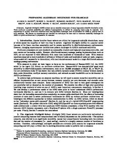
of the off-processor part as well as the communication package and mapping of the original matrix is fairly complex. It depends on the number of ghostlayer points, i.e., those points that are immediate neighbors to a point i, but are located on another processor. Therefore, a large number of ghostlayer points, which can be caused by a non-optimal partitioning, will not only affect communication, but also increase computation. On the other hand, replacing pk MPI tasks by p MPI tasks with k OpenMP threads each that do not require ghostlayer points could lead to improved performance. We evaluate and discuss the number of ghostlayer points for the problems considered here in Section VI-A. Our recent efforts with the AMG code have been aimed at increasing the use of OpenMP in the code. The solve phase, composed primarily of the MatVec and Smoother kernels, can be threaded in a straightforward manner (contiguous subsets of a processor’s rows are operated on by each thread). The setup phase, however, is more complicated and has not been completely threaded. The triple matrix product that forms the coarse-grid operator is threaded. Only a part of the interpolation operators is threaded, since the data structure is not particularly OpenMP friendly. The difficulty is due to the fact that the matrices are compressed and the total number of nonzeros for the operators that need to be generated is not known ahead of time. We currently have no coarsening routine that uses OpenMP, and therefore used the fastest coarsening algorithm available, PMIS, to decrease the time spent in the nonthreaded part of the setup. This algorithm leads to somewhat increased number of iterations and decreased scalability compared to other coarsening algorithms [14]. III. T EST PROBLEMS We use two test problems for our performance study. The first is a 3D Laplace problem on a box with Dirichlet boundary conditions with a seven-point stencil generated by finite differences. We refer to this problem as “Laplace”. The box consists of N × N × αN gridpoints, with α = 1 on Hera and Intrepid, but α = 0.9 on Jaguar, to allow more optimal partitioning when using 6 or 12 threads per node. Assuming mx my mz MPI tasks we partition the domain into subdomains of size mNx × mNy × αN mz . When using the hybrid programming model the work on these subdomains is then divided among OpenMP threads. We designed a second problem to represent a wider range of applications. This problem is a 3D diffusion problem on a more complicated grid. The 2D projection of this grid is shown in Figure 2 (the grid extends equally out of the page in the third dimension with 4 points). We refer to this problem as “MG” because of the shape of the grid. This problem has jumps as well as anisotropies, which appear in many applications. The finite difference stencils for each of the eight parts of the grid are given in the figure as well. In particular, part 7 is anisotropic, and there are jumps between parts 0-3 in the “M” part of the grid. Each part has 48 grid points. This grid can then be further refined by refinement factors Rx , Ry , and Rz in each direction to generate large problems for many processors.

4 0

2

1

B. Dual Hex-Core Cray XT-5 (Jaguar)

5

3

7 6

-1 -1 0:

0

4

0

1:

-1 -1

0

-100 -100 400 0

-100 -100

-1 4 : -1 4 -1 0 -1

-1 5,6 : -1 4 -1 -1

-0.1 2 : -0.1 0.4 -0.1 0

3:

0

-1 -1 4 0

-1 -1

-0.1

-10 7 : -0.1 20.2 -0.1 -10

Fig. 2: The “MG” test problem grid and its associated finite difference stencils. For all test runs presented in this paper, we set Rx = 12px , Ry = 12py , and Rz = 12pz , where px py pz is the number of cores per part, and the total number of cores is 8px py pz . The grids used to generate these two problems have a significantly different geometry. While the Laplace grid is more compact with a (near) optimal surface to volume ratio, the MG grid (as illustrated in Figure 2) is more drawn out and hence has a large overall surface. This impacts the number of processes computing surface elements with fewer numbers of neighbors. We study these two different problems, since the shape can have a significant impact on the communication properties and may also impact scalability. IV. M ULTICORE ARCHITECTURES We study the performance of AMG on three widely different architectures: a traditional multi-core, multi-socket cluster connected by Infiniband (Hera), a Dual-Hex Core Cray XT-5 with a custom 3D torus/mesh network (Jaguar), and a Quadcore BlueGene/P architecture with a custom 3D torus network (Intrepid). A. Quad-Core/Quad-Socket Opteron Cluster (Hera) Our first test machine is a traditional multi-core/multi-socket cluster solution at Lawrence Livermore National Laboratory named Hera. It consists of 864 diskless nodes interconnected by Quad Datarate (QDR) Infiniband (accessed through a PCIe card). Each node consists of four sockets, each equipped with an AMD Quadcore (8356) 2.3 GHz processor. Each core has its own L1 and L2 cache, but the 2 MB L3 cache is shared by all four cores located on the same socket. Each processor provides its own memory controller and is attached to a fourth of the 32 GB memory per node. Accesses to memory locations served by the memory controller on the same processor are satisfied directly, while accesses through other memory controllers are forwarded through the Hypertransport links connecting the four processors. Therefore, depending on the location of the memory, this configuration results in nonuniform memory access (NUMA) times. Each node runs CHAOS 4, a high-performance computing, yet full featured Linux variant based on Redhat Enterprise Linux. All codes are compiled using Intel’s C and OpenMP/C compiler (Version 11.1) and use MVAPICH over IB as the MPI implementation.

Our second test platform is the Cray XT-5 system Jaguar 1 installed at Oak Ridge National Laboratory. It consists of 18,688 nodes organized in 200 cabinets. Each node is equipped with two sockets holding an AMD Opteron Hex-core processor each, as well as 16 GB of main memory split between the two memory controllers of the two sockets, leading to a similar NUMA architecture as seen on Hera. The nodes of the XT-5 are connected with a custom network based on the SeaStar 2+ router. The network is constructed as 3D torus/mesh with wrap-around links (torus-like) in two dimensions and without such links (mesh-like) in the remaining dimension. All applications on Jaguar use a restricted subset of Linux, called Compute Node Linux (CNL). While it provides a Linux like environment, it only offers a limited set of services. On the upside, it provides a lower noise ratio due to eliminated background processes. The scheduler on the Cray XT-5 aims at a compact allocation of the compute processes on the overall network, but if such a compact partition is not available, it will also combine distant nodes (w.r.t. network hops) into one partition. We used PGI’s C and OpenMP/C compilers (v 9.04) and experimented with the OpenMP setting -mp=numa to enable optimizations for NUMA architectures (which mainly consist of preemptive thread pinning as well as localized memory allocations). Further, we used Cray’s native MPI implementation, which is optimized for the SeaStar network. C. Quad-Core Blue Gene/P Solution (Intrepid) The final target machine is the tightly integrated Intrepid Blue Gene/P system at Argonne National Laboratory. This system consists of 40 racks with 1024 compute nodes each and each node contains a quad-core 850 MHz PowerPC 450 Processor bringing the total number of cores to 163,840. In contrast to the other two systems, all four cores have a common and shared access to the complete main memory of 2 GB. This guarantees a uniform memory access (UMA) characteristics. All nodes are connected by a 3D torus network and application partitions are always guaranteed to map to an electrically isolated proper subset of the nodes organized as a complete torus with wrap-around in all three dimensions. On the software side, BG/P systems use a custom compute node kernel with which all applications must link. This kernel provides only the most basic support for the application runtime. In particular, it only supports at most one thread per core, does not implement preemption support, and does not enable the execution of concurrent tasks. The latter has the side effect that executions are virtually noise free. All major functionality, in particular network access and I/O, is function shipped, i.e., remotely executed on a set of dedicated I/O nodes associated with each partition. We compiled all codes using IBM’s C and OpenMP/C compilers v9.0 and used IBM’s MPICH2-based MPI implementation for communication. 1 Precisely,

we are using Jaguar-PF, the newer XT-5 installation at ORNL.

V. P ERFORMANCE RESULTS In this section we present the performance results for BoomerAMG on the three multicore architectures and discuss the notable differences in performance. On each machine, we investigate an MPI-only version of AMG, a version that uses OpenMP across all cores on a node and MPI for inter-node communication, as well as intermediate versions that use a mix of MPI and OpenMP on node. For each experiment, we utilize all available cores per node on the respective machine. We look at the AMG setup times and either the AMG solve time or AMG cycle time (the latter is used for the Laplace problem, where the number of iterations to convergence varies across experimental setups from 17 to 44). We use the following notation for our experiments: “MPI” and “Hmxn”. “MPI” labels indicate timings using an executable that was compiled using MPI only. All other runs were performed using an executable compiled with both MPI and OpenMP and are denoted “Hmxn”, using m MPI tasks per node with n OpenMP threads per MPI process, i.e., “H2x8” translates to the use of 2 MPI tasks per node with 8 OpenMP threads each. In addition, for Hera, which is a NUMA system, we include an optimized OpenMP version that we developed after careful analysis of the initial results. This optimized version, labeled “HmxnMC” in the figures, is described and discussed in detail in Section VI-C (and is, therefore, not discussed in this section). For Jaguar, and for Intrepid, we are presenting a few results using two different partitionings for the MG problem. The more optimal partitioning is denoted with “Hmxnopt” and is discussed in more detail in Section VI-A.

TABLE I: Timings (in seconds) for the MG-2 Problem on Hera. Setup Solve

Procs 256 2048 256 2048

MPI 2.3 25.1 2.0 4.2

H8x2 1.5 6.5 1.9 3.1

H4x4 1.5 2.7 1.9 2.3

H2x8 2.2 3.0 3.7 4.3

H1x16 3.8 5.1 7.3 8.2

H1x16MC 3.8 5.1 2.7 3.3

16 MPI tasks per node, the code creates a high aggregated messaging rate across each node leading to a high pressure on the Infiniband network card, which further increases with growing node count. The commodity Infiniband interconnect is simply not well-suited for this kind of traffic and hence turns into a bottleneck, causing an overall slowdown. In the setup phase, H4x4, corresponding to a single MPI task per socket, initially obtains the best performance since it maps well to the machine architecture. However, for the largest node count it is surpassed by H2x8, which can again be attributed to the network and the higher messaging rate needed to sustain the larger number of MPI processes and with that communication partners in the H4x4 configuration as compared to H2x8. The solve phase is less complex than the setup and mainly depends on the MatVec kernel. Its MPI performance (Figures 3b and 3d) is significantly better, and the OpenMP onnode version performs worst. This poor performance can be directly attributed to the underlying machine architecture and its NUMA properties, and we will discuss this, as well as a solution to avoid this performance penalty, in more detail in Secton VI-C.

A. Hera: AMD Opteron Quad-core We investigate the performance of AMG-GMRES(10) on the Laplace and MG problems on the Hera cluster. For the Laplace problem, we obtained weak scaling results with 100× 100 × 100 grid points per node on up to 729 nodes (11664 cores). We scaled up the problem setting px = py = 2p and pz = 4p leading to 16p3 cores with p = 1, ..., 9. The AMGGMRES(10) setup and cycle times for the Laplace problem are given in Figures 3a and 3b, respectively. Recall that Hera has four quad-core processors per node, and we use all 16 cores on each node for all experiments. We looked at two slightly different variants for the MG problem: MG-1 and MG-2. For the MG-1 problem, we ran on up to 512 nodes (8192 cores) with 1,327,104 grid points per node (82,944 per core), with px = py = 2p and pz = 4p, for p = 1, 2, 3. AMG-GMRES(10) setup and solve times for the MG-1 problem are given in Figures 3c and 3d. For the MG-2 problem, we ran on up to 128 nodes (2048 cores), with px = py = 4p and pz = 2p, with p = 1, 2. Because the results for MG-2 are similar to MG-1, we simply list the MG-2 results in Table I. First we examine the setup phase for both problems (Figures 3a and 3c). The eye-catching trend in these figures is the extremely poor performance for the MPI-only programming model. The algorithms in the setup phase are complex and contain a large amount of non-collective communication. With

B. Jaguar: Cray XT5, AMD Opteron hex-core On Jaguar, we slightly changed the Laplace problem and the MG problem to enable the use of 6 and 12 threads. For the Laplace problem we chose Nx = Ny = 100p, Nz = 90p, px = py = 4p, and pz = 3p, leading to 75,000 grid points per core. We solved this problem for p = 2, 4, 6, ..., 16. We show the resulting setup times in Figure 4a and the cycle times in Figure 4b. For the MG problem, we used px = py = 4p, and pz = 3p with p = 1, 2, 4, 8. Note that MG consists of 8 parts, and therefore the total number of cores required is 8px py pz , leading to runs with the same number of cores as the Laplace problem, but larger numbers of grid points per core. For the MG problem, we also include timings for runs with more optimal partitionings for H2x6 and H4x3. H4x3opt is clearly superior to H4x3, whereas timings for H2x6 are very similar to those of H2x6opt, with H2x6opt being barely better for the problems sizes considered here. For more details on the partitionings, see Section VI-A. For the smaller problem sizes (384, 3072, and for the MG problem, 24576), the results are comparable to those on Hera, which is not surprising, since both machines are NUMA architectures and are based on a similar multi-socket/multi-core node design. However, Jaguar features a custom interconnection network designed for higher messaging rates than the Infiniband interconnect on Hera, allowing significantly better performance for one

0.4

40

0.35

35

0.3

25

MPI

20

H8x2

H4x4

15

Seconds

Seconds

30

H2x8

10

H8x2

0.2

H4x4

0.15

H2x8 H1x16

0.1

H1x16 H1x16MC

5

MPI

0.25

H1x16MC

0.05 0

0 0

2000

4000

6000

8000

10000

0

12000

2000

(a) Setup times for AMG-GMRES(10) on the Laplace problem.

6000

8000

10000

12000

(b) Cycle times for AMG-GMRES(10) on the Laplace problem.

45

10

40

9

35

8

MPI

25

H8x2

20

H4x4

15

H2x8

10

H1x16 H1x16MC

5 0

Seconds

30 Seconds

4000

No. of cores

No. of cores

7

MPI

6

H8x2

5

H4x4

4

H2x8

3

H1x16

2

H1x16MC

1 0

0

2000

4000

6000

8000

No. of cores

(c) Setup times for AMG-GMRES(10) on the MG-1 problem.

0

2000

4000

6000

8000

No. of cores

(d) Solve times for AMG-GMRES(10) on the MG-1 problem.

Fig. 3: Timings on Hera; Hmxn denotes runs performed with m MPI tasks per cluster and n OpenMP threads per MPI task, HmxnMC denotes runs using the MCSup library; “MPI” denotes runs performed with the MPI-only version using 16 MPI tasks per node thread per process cases. The poor performance for H1x12, exhibited when using 384 cores for the MG-problem, can be attributed to NUMA effects. For the MG problem and also for the small Laplace problem runs, the best times are obtained when assigning 1 or 2 MPI tasks per socket. Generally H2x6 or H2x6opt (analog to H4x4 on Hera) achieve the best timings, except for the MG setup, where H4x3opt is the fastest. Here, H4x3opt benefits from an optimal partitioning as well as larger parallelism in the nonthreaded portions of the setup phase. For the Laplace problem, the best setup times are achieved with H1x12 and H2x6, and while H2x6 performs best for the smaller problem sizes, H1x12 is fastest for the large problem sizes. For large sizes of the Laplace problem, timings improve with increasing thread sizes. C. Intrepid: IBM BG/P Quad-core Blue Gene/P systems like Intrepid provide only a restricted operating system environment with a static task distribution. Codes can be run in one of three modes, Symmetric MultiProcessing (SMP), Dual (DUAL), and Virtual Node (VN), and the mode determines the number of possible MPI tasks and threads. In SMP mode, we execute a single MPI process and use four threads per node (labeled “H1x4”); in DUAL mode we use two MPI processes with two threads each (“H2x2”);

and in VN mode, we use four MPI tasks per node with a single thread each. For the latter configuration we run with two binaries, an MPI-only code compiled without OpenMP (“MPI”) and the OpenMP code executed with a single thread (labeled “H4x1”). We scaled up the Laplace problem on Intrepid with 250,000 grid points per node on up to 32,000 nodes (128,000 cores) setting px = py = 2p and pz = 4p, as on Hera, leading to 16p3 cores with p = 2, 4, 8, 12, 16, 20. The results for the AMG-GMRES(10) setup and cycle time (Figures 5a and 5b, respectively) show that the MPI-only model is generally the best-performing for the setup phase, although the solve cycle times are quite similar. This result is in stark contrast to the experiments on Hera, where the MPI-only model shows a significantly higher overhead. This is caused by the custom network on the BG/P system, which is designed to allow higher messaging rates. Overall, we see a good weak scaling behavior; only the times on 27,648 and 128,000 cores using 1 thread per MPI task are slightly elevated due to the less optimal processor geometries compared to the 65,538 and 8192 core runs, which are both powers of two. We do see more variation in the results in the setup phase than in the solve phase, and the

9

0.25

8 0.2

7

MPI

5

H12x1

4

H1x12

3

H4x3

2

H2x6

Seconds

Seconds

6 0.15

MPI H12x1 H1x12

0.1

H4x3 H2x6

0.05

1 0

0

0

50000

100000

150000

200000

0

9

100000

150000

200000

4.5

8

4

7

3.5

6

MPI

5

H12x1 H1x12

4

H4x3

3

H2x6

2

H4x3opt

1

H2x6opt

0

3 Seconds

Seconds

50000

No. of cores (b) Cycle times for AMG-GMRES(10) on the Laplace problem.

No. of cores (a) Setup times for AMG-GMRES(10) on the Laplace problem.

MPI H12x1

2.5

H1x12

2

H4x3

1.5

H2x6

1

H4x3opt

0.5

H2x6opt

0

0

5000

10000

15000

20000

25000

No. of cores (c) Setup times for AMG-GMRES(10) on the MG problem.

0

5000

10000

15000

20000

25000

No. of cores

(d) Solve times for AMG-GMRES(10) on the MG problem.

Fig. 4: Timings on Jaguar: Hmxn denotes runs performed with m MPI tasks per cluster and n OpenMP threads per MPI task, Hmxnopt denotes runs with optimal partitionings, “MPI” denotes runs performed with the MPI-only version using 12 MPI tasks per node. “H1x4” case is the clearly worst performing, while the “H2x2” and “MPI” experiments are quite similar. The “H2x2” case partition has the advantage of each MPI task subdomain being a perfect cube. The slower “H1x4” performance in the setup is likely due to the fact that the percentage of time spent in the nonthreaded portion of the setup phase increases with increasing number of threads as well as due to overhead associated with threading. Now we take a closer look at the scaling results for the two variants of the MG problem. For the MG-1 problem, we ran on up to 16,384 nodes (65,536 cores) with 331,776 grid points per node (82,944 per core), setting px = py = 2p and pz = 4p, with p = 1, 2, 4, 8, as on Hera, and results for the setup and solve phase are given in Figures 5c and 5d. For the MG-2 problem, we ran on up to 32,768 nodes (131,072 cores) with 331,776 grid points per node, with px = py = 4p, pz = 2p, and p = 1, 2, 4, 8, and results for the setup and solve phase are given in Figures 5e and 5f. We see that the MPI-only model is the best-performing. Again, the differences in the solve phase are less pronounced than in the more-complex setup phase. Notice that for the MG-

1 problem, the setup is considerably more expensive for the “H1x4” case. Using a better partitioning for the “H1x4opt” case we were able to get runtimes comparable to the “H2x2” mode. We will further discuss the importance of the choice of partitioning in Section VI-A. “H2x2” is also more expensive than “MPI” in the setup, unlike for the Laplace problem, where the “H2x2” case has a more favorable partitioning. On Intrepid, the fact that the setup phase is not completely threaded becomes very obvious, and we will discuss this further in Section VI-E. VI. L ESSONS LEARNED The measurements presented in the previous section reflect the performance of a production quality MPI code with carefully added OpenMP pragmas. It hence represents a typical scenario in which many application programmers find themselves when dealing with hybrid codes. The partly poor performance shows how difficult it is to deal with hybrid codes on multicore platforms, but it also allows us to illustrate lessons we learned, which help in optimizing the performance of AMG as well as other codes.

A. Effect of Ghostlayer Sizes As mentioned in Section II, the manner in which a problem is partitioned among tasks and threads has an effect on the number of ghostlayer points. Here we evaluate the number of ghostlayer points for each MPI task for both test problems and then analyze the effect of using threading within MPI tasks. We consider only ghostlayer points in the first layer, i.e., immediate neighbor points of a point i that are located on a neighbor processor. Note that this analysis only applies to the first AMG level, since the matrices on coarser levels will have larger stencils, but fewer points within each MPI task. However, since we aggressively coarsen the first grid, leading to significantly smaller coarse grids, the evaluation of the finest level generally requires the largest amount of computation and should take more than half of the time. (Note that this is the case on Intrepid, but not on Hera where network contention leads to large times on the coarse levels.) Also, choosing a nonoptimal partitioning for the MPI tasks will generally lead to nonoptimal partitionings on the lower levels. Let us first consider the Laplace problem. Recall that there are px py pz cores and a grid of size N × N × αN . There are mx my mz MPI tasks. Since we want to also consider OpenMP pk threads, we introduce parameters sk , with sk = m . Now the k number of threads per MPI task is s = sx sy sz . We can define the total number of ghostlayer points for the Laplace problem by adding the surfaces of all subdomains minus the surface of the whole grid: νL (s) = 2(

py px pz + α + α − 1 − 2α)N 2 . sz sy sx

(1)

On Intrepid, α = 1, and px = py = 2p, and pz = 4p. We are interested in the effect of threading on the ghostlayer points for large runs, since future architectures will have millions or even billions of cores. In particular, if p becomes large, and with it N , the surface of the domain becomes negligible, and we get the following result that we refer to as the “ghostlayer ratio”: ρL (s) = lim

p→∞

νL (1) 2 1 1 = 4/( + + ). νL (s) sz sy sx

TABLE II: Ghostlayer ratios on Hera and Intrepid ( up to 4 threads) for thread choices (sx , sy , sz ) Laplace 1.33 (1,1,2) 1.60 (1,1,4) 2.00 (1,2,4) 2.67 (2,2,4)

MG-1 1.17 (1,1,2) 1.28 (1,1,4) 1.73 (1,2,4) 2.34 (2,2,4)

MG-1-opt 1.54 (1,2,2)

MG-2 1.17 (1,2,1) 1.54 (1,2,2) 1.82 (1,4,2) 2.52 (2,4,2)

TABLE III: Ghostlayer ratios on Jaguar for thread choices (sx , sy , sz ) Laplace 1.38 (1,2,1.5) 1.82 (2,2,1.5) 2.22 (2,2,3 )

MG-J 1.24 (1,1,3) 1.66 (1,2,3) 2.21 (2,2,3)

MG-J-opt 1.43 (1,2,1.5) 1.82 (2,2,1.5)

MG problem is given by νM G (s)

=

1152[24( +(25

py pz − 1)px py + (34 − 30)px pz sz sy

px − 8)py pz ]. sx

We can now compute the ratios of all three versions of the MG-problem: ρM G−1 (s) = ρM G−2 (s) = ρM G−J (s) =

83 24 sz

+

34 sy

+

25 sx

.

(4) In Tables II and III we list ratios we get for the choices of sx , sy and sz , that we used in our experiments, as well as (sx , sy , sz ). Note that when using the same number of threads, a larger ratio is clearly correlated to better performance as is obvious when comparing e.g. the performance of MG-1 with that of MG-1-opt in Figure 5c. Hence, it is necessary to choose an appropriate partitioning for each number of threads that optimizes this ghostlayer ratio. However, optimizing this ratio alone is not sufficient to achieve the best performance since other architectural properties, such as socket distributions and NUMA properties, have to be taken into account as well.

(2)

On Jaguar, we chose somewhat different sizes so that the numbers can be divided by 6 and 12. Here, Nx = Ny = N , Nz = 0.9N , px = py = 4p, and pz = 3p. Inserting these numbers into Equation 1, one obtains the following ratio for Jaguar 6 6 5 + ). (3) ρJL (s) = 17/( + sz sy sx The MG problem is generated starting with the grid given in Figure 2, and its uniform extension into the third dimension. Recall that it consists of eight parts with nix × niy × nz points each, i = 0, ..., 7, with nz = 4 and the nix and niy as shown in Figure 2. It then is further refined using the refinement factors Rx = 12px , Ry = 12py and Rz = 12pz , requiring 8px py pz cores. The total number of ghostlayer points for the

B. Network Performance vs. On-node Performance AMG, as with many of its related solvers in the hypre suite [17], is known to create a large amount of small messages. While messages are combined such that a processor contacts each neighbor processor a single time per solve level, the large number of small messages is due to the increased stencil size (and therefore increased number of communication pairs) on the coarser grid levels as discussed in Section II. Consequently, AMG requires a network capable of sustaining a high messaging rate. This situation is worsened by running multiple MPI processes on a single multi-socket and/or multicore node, since these processes have to share network access, often through a single network interface adapter. We clearly see this effect on Hera, which provides both the largest core count per node and the weakest network: on this platform the MPI-only version shows severe scaling

limitations. Threading can help against this effect since it naturally combines the message sent from multiple processes into a single process. Consequently, the H4x4 and H2x8 versions on this platform provide better performance than the pure MPI version. On the other two platforms, the smaller per node core count and the significantly stronger networks that are capable of supporting larger messaging rates, allow us to efficiently run the MPI-only version at larger node counts. However, following the expectations for future architectures, this is a trend that we are likely unable to sustain: the number of cores will likely grow faster than the capabilities of the network interfaces. Eventually a pure MPI model, in particular for message bound codes like AMG, will no longer be sustainable, making threaded codes a necessity. C. Correct Memory Associations and Locality In our initial experiments on the multicore/multi-socket cluster Hera we saw a large discrepancy in performance between running the same number of cores using only MPI and running with a hybrid OpenMP/MPI version with one process per node. This behavior can be directly attributed to the NUMA nature of the memory system on each node: in the MPI-only case, the OS automatically distributes the 16 MPI tasks per node to the 16 cores. Combined with Linux’s default policy to satisfy all memory allocation requests in the memory that is local to the requesting core, all memory accesses are executed locally and without any NUMA latency penalties. In the OpenMP case, however, the master thread allocates the memory that is then shared among the threads. This leads to all memory being allocated on a single memory bank, the one associated with the master thread, and hence to remote memory access penalties as well as contention in the memory controller responsible for the allocations. To fix this, we must either allocate all memory locally in the thread that is using it, which is infeasible since it requires a complete rewrite of most of the code to split any memory allocation to per thread allocations, or we must overwrite the default memory allocation policy and force a distribution of memory across all memory banks. The latter, however, requires an understanding of which memory is used by which thread and a custom memory allocator that distributes the memory based on this information. For this purpose, we developed a multicore support library, called MCSup, which provides a set of new NUMA-aware memory allocation routines to allow programmers to explicitly specify which threads use particular regions of the requested memory allocation. Each of these routines provides the programmer with a different pattern of how the memory will be used by threads in subsequent parallel regions. Most dominant in AMG is a blocked distribution, in which each thread is associated with a contiguous chunk of memory of equal size. Consequently, MCSup creates a single contiguous memory region for each memory allocation request and then places the pages according to the described access pattern.

MCSup first detects the structure of the node on which it is executing. Specifically, it determines the number of sockets and cores as well as their mapping to OpenMP threads, and it then uses this information, combined with the programmer specified patterns, to correctly allocate the new memory. MCSup itself is implemented as a library that must be linked with the application. It uses Linux’s numalib to get low level access to page and thread placement; the programmer has only to replace the memory allocations intended for cross thread usage with the appropriate MCSup routines. The figures in Section V-A show the results obtained when using MCSup (labeled “MC”): with MCSup, the performance of OpenMP in the solve phase is substantially improved. We note that in the setup phase the addition of MCSup had little affect on the OpenMP performance because the setup phase algorithms are such that we are able to allocate the primary work arrays within the threads that use them (as opposed to allocation by the master thread as is required in the solve phase). Overall, though, we see that the performance with MCSup now rivals the performance of MPI-only codes. We see a similar trend on Jaguar: with its dual socket node architecture, it exhibits similar NUMA properties as Hera for runs with 12 threads per core. However, compared to Hera the effect is smaller since each node only has two cores instead of four. This decreases the ratio of remote to total memory accesses and reduces the number of hops remote loads have to take on average. In some cases, like the cycle times for the Laplace problem when run on more than 24K cores, the performance of the 12 thread case is even better than other configurations despite the impact of the NUMA architecture. At these larger scales the smaller number of MPI processes per node, and with that the smaller number of nodes this node exchanges messages with, reduces the pressure onto the NIC to a point where the NUMA performance penalty is less than the penalty caused by the contention for the NIC with four or more MPI processes per node. Applying similar techniques as the ones used in MCSup could theoretically improve performance further, but such implementations would have to get around the limitations of the restricted compute node kernels run on the Cray XT backend nodes. In the future, it is expected that programming models like OpenMP will include features similar to those of MCSup. In particular for OpenMP, such extensions are already being discussed in the standardization process for the next major version of the standard. While this makes external layers like MCSup unnecessary, the main lesson remains: the programmer needs to explicitly describe the association between threads and the memory on which they work. Only with such a specification of memory affinity is it possible to optimize the memory layout and to adjust it to the underlying architecture. D. Per Socket Thread and Process Pinning The correct association of memory and threads ensures locality and the avoidance of NUMA effects only so long as this association does not change throughout the runtime of the program. None of our two NUMA platforms actively migrates

TABLE IV: Timings (in seconds) for the MG-1 Problem with 10,616,832 grid points on Intrepid on 32 nodes.

Setup

Solve

Programming model MPI-only MPI-OMP Speedup MPI-only MPI-OMP Speedup

128 MPI tasks 2.0 2.5 0.80 3.8 3.8 1.00

64 MPI tasks 4.3 4.0 1.08 7.4 4.1 1.80

32 MPI tasks 11.6 7.1 1.63 14.7 4.3 3.42

memory pages between sockets, but on the Hera system with its full featured Linux operating system, thread and processes can be scheduled across the entire multi-socket node, which can destroy the carefully constructed memory locality. It is therefore necessary to pin threads and processes to the appropriate cores and sockets so that the memory/thread association determined by MCSup is maintained throughout the program execution. Note that MCSup’s special memory allocations are only required when the threads of a single MPI process span multiple sockets; otherwise, pinning the threads of an MPI process to a socket is sufficient to guarantee locality, which we clearly see in the good performance of the H4x4 case on Hera. E. Performance Impact of OpenMP Constructs As we mentioned earlier, while the solve phase is completely threaded, some components of the setup phase do not contain any OpenMP statements, leading to a decrease in parallelism when using more than one thread per MPI task. Therefore, one would expect the overall performance of the setup time to deteriorate, particularly when increasing the number of OpenMP threads and thus decreasing number of MPI tasks. Interestingly, this appears not to be the case on Hera and Jaguar. On Hera, network contention caused by large numbers of MPI tasks appears to overpower any potential performance gain through increased parallelism. On Jaguar it appears that using the correct configuration to match the architecture, i.e., using one or two MPI tasks per socket and 6 or 3 threads per MPI task, is more important. However, the decreased parallelism becomes very obvious on Intrepid. To get a better idea of the effect of the lack of OpenMP threads in some components of the setup phase, we listed timings for both phases of the MG-1 problem run on 32 nodes in Table IV. The ’MPI-only’ line lists the times for solving MG-1 in MPIonly mode using 128, 64 and 32 cores. The ’MPI-OMP’ line beneath lists the times for solving the same problem with 128, 64 and 32 MPI tasks and 1,2, and 4 threads, respectively, such that all 128 cores are utilized. We also list the speedup that is obtained by using OpenMP vs. no OpenMP. One can clearly see the time improvement achieved by using two or four threads within each MPI task for the solve phase. However, as expected, the speedups for the setup phase portions are very small due to the nonthreaded portions of code. Also note that the use of OpenMP with one thread shows a 25% overhead in the more complex setup phase, whereas the solve phase performance is similar. Since the

Region 3 No OMP OMP for loop OMP for no priv. OMP par. region OMP reg. no priv.

Time (s) 20.09s 29.33s 29.35s 29.54s 23.32

Rel. time 100% 146% 146% 147% 116%

Loads 100% 138% 137% 146% 107%

Branches 100% 150% 148% 152% 103%

Region 4 No OMP OMP for loop OMP for no priv. OMP par. region OMP reg. no priv.

Time (s) 42.60s 52.29s 52.41s 55.80s 46.92

Rel. time 100% 123% 123% 131% 110%

Loads 100% 119% 119% 121% 98%

Branches 100% 132% 133% — 98%

TABLE V: Cumulative timings and hardware counter data for two OpenMP regions in hypre_BoomerAMGBuildCoarseOperator comparing code versions without OpenMP (baseline) to using an OpenMP for loop and an OpenMP parallel region each with and without private variables (128 MPI tasks, 1 thread per task, BG/P, problem MG-1)

thread configuration is the same for those two versions, this overhead must stem from the OpenMP runtime system. We traced the overhead back to a single routine in the setup phase — hypre_BoomerAMGBuildCoarseOperator. This routine computes a triple matrix product, and it contains four OpenMP for regions, each looping over the number of threads, with regions three and four dominating the execution time. The timings for those regions along with the number of data loads and branch instructions are shown in Table V. The code of this function describes the (complex) setup of the matrix. It was manually threaded and uses a for loop to actually dispatch this explicit parallelism. However, we can replace the more common for loop with an explicit OpenMP parallel region, which implicitly executes the following block once on each available thread. While the semantics of these two constructs in this case is equivalent, the use of a parallel region slightly slows the execution, in particular in region 4. Further, we find that both regions use a large number of private variables. While these are necessary for correct execution in the threaded case, we can omit them in the single thread case. This change has no impact on the code using an OpenMP for loop, but when removing private variables from the OpenMP parallel regions, the performance improves drastically from 47% to 16% overhead for region 3 and 31% to 10% for region 4. We can see these performance trends also in the corresponding hardware performance counter data, also listed in Table V, in particular the number of loads and the number of branches executed during the execution of these two regions. This is likely attributable to the outlining procedure and the associated changes in the code needed to privatize a large number of variables, as well as additional book keeping requirements. Based on these findings we are considering rewriting the code to reduce the number of private variables, so that this performance improvement will translate to the threaded case.

VII. C ONCLUSIONS This paper presents a comprehensive study of a state-ofthe-art Algebraic Multigrid (AMG) solver on three large scale multi-core/multi-socket architectures. These systems already cover a large part of the HPC space and will dominate the landscape in the future. Good and (even more important) portable performance for key libraries, like AMG, on such systems will therefore be essential for their successful use. However, our study shows that we are still far from this goal, in particular with respect to performance portability. The discussion in the previous section illustrates the many pitfalls that await developers of hybrid OpenMP/MPI codes. In order to achieve at least close to optimal performance, particularly on NUMA systems, it is essential not only to guarantee memory locality, but also to optimize domain partitioning for each thread count. Further, in order to maintain this locality, it is advisable to turn off any thread or process migration across sockets; threads of an MPI process should always be kept on the same socket to achieve both memory locality and to minimize OS overhead. Further, as the example in Section VI-E shows, it is imperative to select the correct OpenMP primitive for a particular task, especially if multiple, equivalent pragmas are available. Finally, it is important to reduce the number of private variables, since they can incur additional bookkeeping overhead. Overall, our results show that the performance and scalability of AMG on the three multicore architectures is varied, and a general solution for obtaining good multicore performance is not possible without considering the specific target architecture including node architecture, interconnect, and operating system capabilities. In many cases it is left to the programmer to find the right techniques to extract the optimal performance and the choice of techniques is not always straightforward. With the right settings, however, we can achieve a performance for hybrid OpenMP/MPI solutions that is at least equivalent to the existing MPI model, but with the promise of scalability to concurrency levels that would not be possible for MPI-only applications. VIII. ACKNOWLEDGMENTS This work was performed under the auspices of the U.S. Department of Energy by Lawrence Livermore National Laboratory under contract DE-AC52-07NA27344 (LLNL-CONF458074). It also used resources of the Argonne Leadership Computing Facility at Argonne National Laboratory, which is supported by the Office of Science of the U.S. Department of Energy under contract DE-AC02-06CH11357, as well as resources of the National Center for Computational Sciences at Oak Ridge National Laboratory, which is supported by the Office of Science of the U.S. Department of Energy under Contract No. DE-AC05-00OR22725. These resources were made available via the Performance Evaluation and Analysis Consortium End Station, a Department of Energy INCITE project. Neither Contractor, DOE, or the U.S. Government, nor any person acting on their behalf: (a) makes any warranty or representation, express or implied, with respect to the

information contained in this document; or (b) assumes any liabilities with respect to the use of, or damages resulting from the use of any information contained in the document. R EFERENCES [1] M. Heroux, “Scalable computing challenges: An overview,” Talk at the 2009 SIAM Annual Meeting, Denver, CO, July 2009. [2] hypre, “High performance preconditioners,” http://www.llnl.gov/CASC/linear solvers/. [3] R. D. Falgout, “An introduction to algebraic multigrid,” Computing in Science and Eng., vol. 8, no. 6, pp. 24–33, 2006. [4] A. H. Baker, M. Schulz, and U. M. Yang, “On the performance of an algebraic multigrid solver on multicore clusters,” in Proceedings of VECPAR 2010, Berkeley, CA, 2010, http://vecpar.fe.up.pt/2010/papers/24.php. [5] J. Ruge and K. St¨uben, “Algebraic multigrid (AMG),” in Multigrid Methods, ser. Frontiers in Applied Mathematics, S. McCormick, Ed., vol. 3. SIAM, 1987. [6] A. Brandt, S. McCormick, and J. Ruge, “Algebraic multigrid (AMG) for sparse matrix equations,” in Sparsity and its Applications, D. J. Evans, Ed. Cambridge: Cambridge University Press, 1984, pp. 257–284. [7] K. St¨uben, “An introduction to algebraic multigrid,” in Multigrid, U. Trottenberg, C. Oosterlee, and A. Sch¨uller, Eds. Academic Press, London, 2001, pp. 413–532. [8] J. Schmidt, G. Berti, J. Fingberg, J. Cao, and G. Wollny, “A finite element based tool chain for the planning and simulation of maxillo-facial surgery,” in ECCOMAS 2004, P. Neittaanmaki, T. Rossi, K. Majava, and O. Pironneau, Eds., 2004. [9] R. Masson, P. Quandalle, S. Requena, and R. Scheichl, “Parallel preconditioning for sedimentary basin simulations,” in LSSC 2003, L. et al., Ed. Springer-Verlag, 2004, vol. 2907, pp. 93–102. [10] E. Chow, R. Falgout, J. Hu, R. Tuminaro, and U. Yang, “A survey of parallelization techniques for multigrid solvers,” in Parallel Processing for Scientific Computing, M. Heroux, P. Raghavan, and H. Simon, Eds. SIAM Series on Software, Environments, and Tools, 2006. [11] U. Yang, “Parallel algebraic multigrid methods – high performance preconditioners,” in Numerical Solution of Partial Differential Equations on Parallel Computers, A. Bruaset and A. Tveito, Eds. Springer-Verlag, 2006, vol. 51, pp. 209–236. [12] H. De Sterck, R. D. Falgout, J. Nolting, and U. M. Yang, “Distancetwo interpolation for parallel algebraic multigrid,” Num. Lin. Alg. Appl., vol. 15, pp. 115–139, 2008. [13] R. Falgout, J. Jones, and U. Yang, “The design and implementation of hypre, a library of parallel high performance preconditioners,” in Numerical Solution of Partial Differential Equations on Parallel Computers, A. Bruaset and A. Tveito, Eds. Springer-Verlag, 2006, vol. 51, pp. 267–294. [14] H. De Sterck, U. M. Yang, and J. Heys, “Reducing complexity in algebraic multigrid preconditioners,” SIMAX, vol. 27, pp. 1019–1039, 2006. [15] U. M. Yang, “On long distance interpolation operators for aggressive coarsening,” Num. Lin. Alg. Appl., vol. 17, pp. 353–472, 2010. [16] R. Falgout, J. Jones, and U. M. Yang, “Pursuing scalability for hypre’s conceptual interfaces,” ACM ToMS, vol. 31, pp. 326–350, 2005. [17] R. Falgout and U. Yang, “hypre: a Library of High Performance Preconditioners,” in Proceedings of the International Conference on Computational Science (ICCS), Part III, LNCS vol. 2331, Apr. 2002, pp. 632–641.

6 0.25

5

0.2

H1x4

H1x4 3

H2x2

2

MPI

1

0.15

H2x2

0.1

MPI

Seconds

Seconds

4

H4x1

0.05

H4x1

0

0

0

25000

50000

75000

100000

125000

0

No of cores (a) Setup times for AMG-GMRES(10) on the Laplace problem.

25000

50000

75000

100000

125000

No of cores (b) Cycle times for AMG-GMRES(10) on the Laplace problem.

20

7

18

6

16 5

12

MPI

10

H2x2

8

H1x4

6

H4x1

4

H1x4opt

Seconds

Seconds

14

MPI

4

H2x2

3

H1x4 H4x1

2

H1x4opt

1

2

0

0 0

10000

20000

30000

40000

50000

60000

0

10000

20000

No of cores

40000

50000

60000

No of cores

(c) Setup times for AMG-GMRES(10) on the MG-1 problem.

(d) Solve times for AMG-GMRES(10) on the MG-1 problem.

14

7

12

6

10

5

MPI

8

H2x2

6

H1x4

4

H4x1

2 0

MPI Seconds

Seconds

30000

4 H2x2 3 H1x4

2 H4x1 1 0

0

25000

50000

75000

100000

125000

No of cores (e) Setup times for AMG-GMRES(10) on the MG-2 problem.

0

25000

50000

75000

100000

125000

No of cores (f) Solve times for AMG-GMRES(10) on the MG-2 problem.

Fig. 5: Timings on Intrepid; Hmxn denotes runs performed with m MPI tasks per cluster and n OpenMP threads per MPI task, Hmxnopt denotes runs with optimal partitionings, “MPI” denotes runs performed with the MPI-only version using 4 MPI tasks per node