Chaos in the Random Field Ising Model

Chaos in the random field Ising model Mikko Alava1,2 and Heiko Rieger3,4 1

arXiv:cond-mat/9804136v1 [cond-mat.dis-nn] 14 Apr 1998

2

NORDITA, Blegdamsvej 17, 2100 Copenhagen, Denmark Helsinki University of Technology, Laboratory of Physics, P.O. Box 1100, 02015 HUT, Finland 3 Institut f¨ ur Theoretische Physik, Universit¨ at zu K¨ oln, 50923 K¨ oln, Germany 4 HLRZ, Forschungszentrum J¨ ulich, 52425 J¨ ulich, Germany (March 18, 1998)

The sensitivity of the random field Ising model to small random perturbations of the quenched disorder is studied via exact ground states obtained with a maximum-flow algorithm. In one and two space dimensions we find a mild form of chaos, meaning that the overlap of the old, unperturbed ground state and the new one is smaller than one, but extensive. In three dimensions the rearrangements are marginal (concentrated in the well defined domain walls). Implications for finite temperature variations and experiments are discussed.

size L, the Jij denote interaction strengths and hi local fields, both quenched random variables obeying some distribution (continuous, in order to exclude ground state degeneracies). The case Jij Gaussian (with mean zero and variance one) and hi = 0 is the spin glass (SG), the case Jij ≥ 0 and hi = 0 is the random bond ferromagnet (RBFM) and the case Jij = J and hi Gaussian (with mean zero and variance hr ) is the random field Ising model (RFIM). In order to study the sensitivity of the ground state of these systems with respect to small changes in the quenched disorder we can apply a random perturbation of amplitude δ ≪ 1 to any of the quenched random variable. As a consequence the new ground state will differ from the old one. The RFIM ground state changes when the domain structure changes (for purely ferromagnetic states this argument does not work). One can estimate when the two ground states will be uncorrelated, beyond a length scale L∗ This can be found considering domain walls with an Imry-Ma [11] type argument [3,9]: The energy Ef lip to flip droplets or domains or excitations of size L scales like Lθ , where θ is the energy fluctuation exponent (θ is denoted y in the SG context [3]). The energy change due to the random perturbation Erand scales like δLd/2 , where d = ds the fractal dimension of the droplet’s surface in the SG case, d = D − 1 the interface dimension in the RBIM and d = D in the RFIM case. The decorrelation takes place when Erand (L) > Ef lip (L), i.e. for L > L∗ ∼ δ −1/λ with λ = d/2 − y. In SG jargon L∗ is called the overlap length and λ is denoted ζ, the chaos exponent [3,7]. Two remarks are in order: first, as pointed out in [9] and [10] already for L < L∗ the ground state is slightly altered by the random perturbation. This is, however, an effect of the interplay between elastic energy and Erand . This leads to displacements of the domain wall of size ∆x ∼ δLα with α = λ + χ, where χ is the roughness exponent. The roughness exponent [12] and the energy fluctuation exponent θ are related via θ = 2χ + D − 3 [9]. The second remark concerns the RFIM-case: for D ≤ 2 the concept of a macroscopic domain wall fails here,

The concept of chaos in disordered systems refers to the sensitivity of their equilibrium state (at finite temperatures) or ground state (at zero temperature) with respect to infinitesimal perturbations. In spin glasses [1] for instance it is well known that small changes of parameters like temperature or external field causes a complete rearrangement of the equilibrium configuration [2,3]. This has experimentally observable consequences like reinitialization of aging in temperature cycling experiments [4] and has also been investigated in numerous theoretical works [5]. A slight random variation of the quenched disorder has the very same effect on the ground state configurations. Although of similar origin, chaos with respect to temperature changes is harder to observe than chaos with respect to disorder changes [6], and the latter phenomena has been used to quantify spin glass chaos in numerical investigations [3,7]. This type of chaos has actually later been discovered in another, simpler random system, the directed polymer in a random medium [8–10], which is equivalent to an dommain wall in a random bond ferromagnet. The interface displacement as a reaction to infinitesimal random changes of bond-strengths obeys particular scaling laws with exponents related to the well-known interface roughness exponent χ [9,10]. In this paper we consider the random field Ising model [1] and study, the first time to our knowledge, the sensitivity of its ground state with respect to small changes in the random field configurations. It turns out that the emerging picture is very reminiscent of chaos in spin glasses and random interfaces. This statement is quantified by the following phenomenological picture [3,9]. Consider a random Ising system defined, for instance, by the Hamiltonian X X h i Si (1) Jij Si Sj − H =− hiji

i

where Si = ±1 are Ising spins, hiji indicates nearest neighbor pairs on a D-dimensional lattice of, say, linear 1

1.00

300 0.99

200

L = 100 L = 500 L = 2000

0.98

q 0.97

100 0.96

0

0.95 0.0

0

100

200

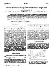
FIG. 1. A ground state plus the perturbation-induced changes. The original spin-orientations are indicated in grey for Si = +1 and white for Si = −1, the flipped spins are indicated in black. L = 320, ∆ = 2 and δ = 0.1 (see text).

1 X Si Si′ (δ) LD i

2.0

∆

3.0

4.0

1.00

and the above considerations can only be transfered cum grano salis. This means that they are sensible only for L ≪ ξ ∼ exp(−h2r /A), the typical size of domains in the 2D RFIM [13,14]. In 3D the situation is different: The concept of a domain wall is well defined and we get with the estimate for the roughness exponent χ = 2/3 [12] and, consequently, θ = 4/3 the result λ = 1/6, i.e. L∗ ∼ δ −1/6 . The typical displacement of a domain wall thus is, as above, ∆x ∼ Lα with α = 2/3 for L ≪ L∗ and α = 5/6 for L ≫ L∗ . If we take the above arguments serious for the RFIM in 2D the overlap length L∗ turns out to be formally infinite (since with θ = 1 one has λ = 0), where one has of course to be careful due to logarithmic corrections to the energy Ef lip . Thus the mechanism by which rearrangements take place is due to the interplay between elastic energy and Erand . Moreover, in the 2D RFIM, the typical displacement of domain walls should scale as ∆x ∼ δL for L ≪ ξ since α = λ+χ = 1. As a conseqence the correlation or overlap between the old, unperturbed, ground state Si and the new one Si′ (δ) q=

1.0

300

0.95

q 0.90

0.85

L = 40 L = 80 L = 160 L = 240 L = 320 1

∆

10

FIG. 2. a) (Top) Scaling of the overlap parameter with random field strength for the 1D spin chain. b) (Bottom) Scaling of the overlap in 2D for the system sizes L = 40,80,160,240 and 320 and for δ = 0.1.

in white and grey, respectively, and the flipped spins in black. There are two features one should note. First, the size of the system is larger than the critical length scale needed for ground state breakup and the magnetization is practically zero. Second, the flipped spins form a number of clusters of varying size, that seem to concentrate on the cluster boundaries of the original groundstate. Figure 2 shows what happens as one sweeps the RFstrength (∆). In arbitrary dimensions, the limit ∆ → ∞ goes over to a site percolation problem, i.e. the local RForientation gives the spin state at a site. In that limit the overlap q is determined by the probability of the applied perturbation δ to change the this orientation. For somewhat smaller fields q gets smaller and in an apparently linear fashion as ∆ changes. In the 1D case the overlap is not sensitive to the system size above a certain thresh-

(2)

behaves like 1 − q ∼ Lα−1 and therefore q should be of order O(1), depending on the probability with which domain wall displacements occur. In what follows we present results of exact ground state calculations for 1D spin chains and for 2D systems. We use a random field distribution and a perturbation distribution that have a constant probability density between −∆ and ∆ and −δ/2 and δ/2, respectively and set Jij = 1. Figure 1 shows an example of a large 2D ground state (L = 320) with the two spin orientations shown 2

6

10

0.4

L = 40 L = 160 L = 320

0

10

0.3

4

n(s)

0.2

δq

P(q)

10

−1

10

2

10

0.1

−2

10

10

100 L

1000 0

0.0

0.2

10

0.4

0.6

0.8

1.0

10

100

1000

10000

s

q

FIG. 4. Cluster size distributions of clusters of flipped spins for δ = 0.1, L = 40, 160, 320, and ∆ = 2.

FIG. 3. Probability distributions of the overlap q for ∆ = 1.8 for the system sizes L = 40 . . . 320. The inset shows the standard deviations of the overlap pdf’s for ∆ = 1.4, 1.6, 1.8, 2, 2.4.

lation yields p(Sn = Sn′ ) = 1 − π1 δr /hr + O(δ 2 ). For the data shown in Fig. 1a, in which h2r = ∆2 /3 and δr2 = δ 2 ∆2 /12 with δ = 0.1, we have δr /hr = 0.05 and hence q = −1+2p(Sr = Sr′ ) ≈ 0.97 agreeing roughly with the numerical results for hr → 0 in the limit L → ∞. The 2D behavior is depicted in Figure 2 for δ = 0.1. The number of simulations is 10000 for L = 40 and 80, 4000 for L = 160, 1000 for L = 240 and 500 for L = 320. The generic behavior of the overlap is as for the 1D chain: q(∆) is roughly linear until the regime of small fields (∆ ≤ 2) after which it seems to saturate to a δ-dependent value q(δ). The cross-overs (increase of q with decreasing ∆) are due to the ground state breakup mechanism. For small systems the ground state is ferromagnetic, except for a limited number of domains of the opposite spin orientation. The decrease in q is caused by the effect of the ground state becoming more and more uniform (magnetization |m| → 1). Otherwise the behavior resembles strongly the 1D case. The thermodynamic behavior of the overlap is also visible in the statistics of overlap distributions. Figure 3 shows how the probability distribution P (q) of q behaves with varying system size and for ∆ = 1.8 (the data is the same as presented in Fig. 2). For all systems P (q) is peaked at q = 1 but as L is increased a peak appears in the distribution, resembling a Gaussian. The inset of Fig. 3 shows the standard deviation δq of P (q) for varying ∆ as a function of the system size L. Except for the bynow standard cross-over for small L and ∆ we observe, that the width of the distribution decreases, which signals that in the thermodynamic limit P (q) approaches a delta-function-like sharp one. The cross-over exponent c, defined with δq ∼ L−c , seems to be exactly one (c = 1). The mechanism by which q is determined is illustrated in Figure 4. The size distribution of flipped clusters n(s) converges with L to a power-law, n ∼ s−1.6 , with a cut-

old in ∆, below which the overlap quickly increases to unity again, which indicates a typical domain size. The overlap seems to become a δ-dependent constant in the thermodynamic limit and for ∆ → 0. This 1D behavior can be understood as follows. For simplicity let us assume that the first spin is fixed to be up, i.e. S0 = +1. Then the random field energy Ptotal n at site n is given by Hr = i=1 hi in the Pnunperturbed system and Hn′ = Hn + ∆n with ∆n = i=1 δi , in the perturbed one. If hi and δi are independently distributed variables with zero mean and variance hr = [h2i ]av and δr = [δi2 ]av , respectively, the variables Hn and ∆n are (for n ≫ 1) Gaussian with mean zero and variance nhr and nδr , respectively. The probability distribution P (Hn , Hn′ ) is simply given by Z P (Hn , Hn′ ) = d∆r P (Hn )P (∆n )δ(Hn + ∆n − Hn′ ) . Now the total RF fluctuations Hn and Hn′ produce domains if their magnitude is large enough to overcome the ferromagnetic coupling: suppose that Si = +1 and Hi > −J for i = 1, . . . n (i.e. a plus-domain), but Hn+1 < −J; then Sn+1 will be flipped, i.e. Sn+1 = −1 and a new (minus-) domain starts. For large enough typical domain sizes the total RF fluctuations become large: one can neglect J and assume that only the sign of Hn and Hn′ determines the ground state (note that this is different from the high field region hn ≫ J, in which the local random fields hi dominate).Thus, the probability for Sn and Sn′ being equal is given by Z p(Sn = Sn′ ) = dHn dHn′ P (Hn , Hn′ ) · θ(Hn · Hn′ ) , (3) where θ is the step function. A straightforward calcu3

1.00

outcome is simply that of a random walk (∆x ∼ L1/2 ). In other words assuming that typical valleys in the energy landscape are separated by an energy given by the energy fluctuation exponent gives completely different results for temperature and ground state chaos than for random bond disorder. This discussion is intimately related to coarsening and ageing in the RFIM; one should note that there are so far no simulation results that address these questions directly.

q

0.95

∆ =1.4 ∆ =1.6 ∆ =1.8 ∆ =2.4

0.90

0.85 0.00

0.02

ACKNOWLEDGMENTS

0.04

δ

0.06

0.08

This work has been performed within the FinnishGerman cooperation project supported by the Academy of Finland and the DAAD. M.A. would like to thank Eira Sepp¨al¨a for a version of the computer code used.

0.10

FIG. 5. Dependence of the overlap q on the perturbation strength δ for weak and strong magnitudes (∆), L = 80.

off that depends very weakly if at all on L. This has to be so for the overlap not to diverge to zero in the thermodynamic limit, since one can write 1 − q as an integral over n(s): a L-dependent cut-off would imply that q would decrease continuously. Finally in Figure 5 we demonstrate that 1 − q ∼ δ for small δ. This follows from the scaling arguments presented for 2D RFIM domain walls and the 1D RF chain. In this paper we have considered the stability of the random field Ising model to small perturbations. Unlike in spin glasses, it turns out that the RFIM ground state shows a weak form of chaos, similar to directed polymers or random bond Ising model domain walls. The overlap q attains its value from fluctuations of domain walls, in both 1D and 2D. Thus the ground state stays almost intact. The ground state domains are robust against external perturbations since,Pmost likely, the field excess of a domain is extensive ( hi ∼ V ). For the RFIM in 3D the prediction of the domain wall scaling argument is that q should converge to unity since the domain wall displacement exponent α here is 5/6: the displacement of a domain wall on large enough length scales is ∆x ∼ Lα and therefore 1−q ∝ Lα−1 → 0. Moreover, in both limits hr /J → 0 and hr /J → ∞, i.e. deep in the ferromagnetic phase and deep in the paramagnetic phase, it is trivial that q → 1. One would like to extend the argumentation to changes in temperature as is common for spin glasses and random bond -type directed polymers. In spin glasses chaos is intimately linked to the non-equilibrium correlation length, which gives rise to measurable consequences in e.g. temperature cycling experiments that measure the out-ofphase susceptibility. Here, however, repeating the scaling argument of domain wall for temperature changes results in a displacement exponent which does not produce any extensive changes in the overlap. In 2D the predicted

[1] See e.g. Spin Glasses and Random Fields, ed. A. P. Young, (World Scientific, Singapore, 1997) for a review. [2] D. S. Fisher and D. A. Huse, Phys. Rev. Lett. 56, 1601 (1986). [3] A. J. Bray and M. A. Moore, Phys. Rev. Lett. 58, 57 (1987). [4] P. Refregier, E. Vincent, J. Hammann, and M. Ocio, J. Physique 46, 1533 (1987); F. Lefloch, J. Hammann, M. Ocio, and E. Vincent, Europhys. Lett. 18, 647 (1992); J. Mattsson et al., Phys. Rev. 47, 14626 (1993); H. Rieger, J. Physique I 4, 883 (1994). [5] F. Ritort, Phys. Rev. B 50, 6844 (1994); J. Kisker, L. Santen, M. Schreckenberg and H. Rieger, Phys. Rev. B 53, 6418 (1996); I. Kondor, J. Phys. A 22, L163 (1989); I. Kondor and A. V´egs¨ o, J. Phys. A 26, L641 (1993); S. Franz and M. Ney-Nifle, J. Phys. A 28, 2499 (1995). [6] M. Ney-Nifle and A. P. Young, J. Phys. A 30, 5311 (1997). [7] H. Rieger, L. Santen, U. Blasum, M. Diehl, M. J¨ unger and G. Rinaldi, J. Phys. A 29, 3939 (1996). [8] Y.-C. Zhang, Phys. Rev. Lett. 59, 2125 (1987). [9] T. Nattermann, Phys. Rev. Lett. 60, 2701 (1988). [10] M. V. Feigel’man and V. M. Vinokur, Phys. Rev. Lett. 61, 1139 (1988). [11] Y. Imry and S.-K. Ma, Phys. Rev. Lett. 35, 1399 (1975). [12] D. S. Fisher, Phys. Rev. Lett. 56, 1964 (1986). [13] K. Binder, Z. Phys. B50, 343 (1983). [14] E. T. Sepp¨ al¨ a, V. Pet¨ aj¨ a, and M. J. Alava, submitted for publication. [15] M. Aizenman and J. Wehr, Phys. Rev. Lett. 62, 2503 (1989). [16] J. Bricmont and A. Kupiainen, Phys. Rev. Lett. 59, 1829 (1987). [17] G. Grinstein and S.K. Ma, Phys. Rev. B38, 2588 (1983).

4