CHAPTER 11 Numerical Differentiation and Integration

CHAPTER 11 Numerical Differentiation and Integration Differentiation and integration are basic mathematical operations with a wide range of applications in many areas of science. It is therefore important to have good methods to compute and manipulate derivatives and integrals. You probably learnt the basic rules of differentiation and integration in school — symbolic methods suitable for pencil-and-paper calculations. These are important, and most derivatives can be computed this way. Integration however, is different, and most integrals cannot be determined with symbolic methods like the ones you learnt in school. Another complication is the fact that in practical applications a function is only known at a few points. For example, we may measure the position of a car every minute via a GPS (Global Positioning System) unit, and we want to compute its speed. If the position is known as a continuous function of time, we can find the speed by differentiating this function. But when the position is only known at isolated times, this is not possible. The same applies to integrals. The solution, both when it comes to integrals that cannot be determined by the usual methods, and functions that are only known at isolated points, is to use approximate methods of differentiation and integration. In our context, these are going to be numerical methods. We are going to present a number of methods for doing numerical integration and differentiation, but more importantly, we are going to present a general strategy for deriving such methods. In this way you will not only have a number of methods available to you, but you will also be able to develop new methods, tailored to special situations that you may encounter. 227

We use the same general strategy for deriving both numerical integration and numerical differentiation methods. The basic idea is to evaluate a function at a few points, find the polynomial that interpolates the function at these points, and use the derivative or integral of the polynomial as an approximation to the function. This technique also allows us to keep track of the so-called truncation error, the mathematical error committed by integrating or differentiating the polynomial instead of the function itself. However, when it comes to roundoff error, we have to treat differentiation and integration differently: Numerical integration is very insensitive to round-off errors, while numerical differentiation behaves in the opposite way; it is very sensitive to round-off errors.

11.1 A simple method for numerical differentiation We start by studying numerical differentiation. We first introduce the simplest method, derive its error, and its sensitivity to round-off errors. The procedure used here for deriving the method and analysing the error is used over again in later sections to derive and analyse additional methods. Let us first make it clear what numerical differentiation is. Problem 11.1 (Numerical differentiation). Let f be a given function that is only known at a number of isolated points. The problem of numerical differentiation is to compute an approximation to the derivative f 0 of f by suitable combinations of the known values of f . A typical example is that f is given by a computer program (more specifically a function, procedure or method, depending on you choice of programming language), and you can call the program with a floating-point argument x and receive back a floating-point approximation of f (x). The challenge is to compute an approximation to f 0 (a) for some real number a when the only aid we have at our disposal is the program to compute values of f . 11.1.1 The basic idea Since we are going to compute derivatives, we must be clear about they are defined. Recall that f 0 (a) is defined by f 0 (a) = lim

h→0

f (a + h) − f (a) . h

(11.1)

In the following we will assume that this limit exists; i.e., that f is differentiable. From (11.1) we immediately have a natural approximation to f 0 (a); we simply 228

pick a positive h and use the approximation f 0 (a) ≈

f (a + h) − f (a) . h

(11.2)

Note that this corresponds to approximating f by the straight line p 1 that interpolates f at a and a − h, and then using p 10 (a) as an approximation to f 0 (a). Observation 11.2. The derivative of f at a can be approximated by f 0 (a) ≈

f (a + h) − f (a) . h

In a practical situation, the number a would be given, and we would have to locate the two nearest values a 1 and a 2 to the left and right of a such that f (a 1 ) and f (a 2 ) can be found. Then we would use the approximation f 0 (a) ≈

f (a 2 ) − f (a 1 ) . a2 − a1

In later sections, we will derive several formulas like (11.2). Which formula to use for a specific example, and exactly how to use it, will have to be decided in each case. Example 11.3. Let us test the approximation (11.2) for the function f (x) = sin x at a = 0.5 (using 64-bit floating-point numbers). In this case we have f 0 (x) = cos x so f 0 (a) = 0.87758256. This makes it is easy to check the accuracy. We try with a few values of h and find h −1

10 10−2 10−3 10−4 10−5 10−6

¡

¢± f (a + h) − f (a) h

E 1 ( f ; a, h)

0.8521693479 0.8751708279 0.8773427029 0.8775585892 0.8775801647 0.8775823222

2.5 × 10−2 2.4 × 10−3 2.4 × 10−4 2.4 × 10−5 2.4 × 10−6 2.4 × 10−7

¡ ¢± where E 1 ( f ; a, h) = f (a)− f (a +h)− f (a) h. In other words, the approximation seems to improve with decreasing h, as expected. More precisely, when h is reduced by a factor of 10, the error is reduced by the same factor.

229

11.1.2 The truncation error Whenever we use approximations, it is important to try and keep track of the error, if at all possible. To analyse the error in numerical differentiation, Taylor polynomials with remainders are useful. To analyse the error in the approximation above, we do a Taylor expansion of f (a + h). We have f (a + h) = f (a) + h f 0 (a) +

h 2 00 f (ξh ), 2

where ξh lies in the interval (a, a + h). If we rearrange this formula, we obtain f 0 (a) −

h f (a + h) − f (a) = − f 00 (ξh ). h 2

(11.3)

This is often referred to as the truncation error of the approximation, and is a reasonable error formula, but it would be nice to get rid of ξh . We first take absolute values in (11.3), ¯ ¯ ¯ 0 ¯ ¯ ¯ ¯ f (a) − f (a + h) − f (a) ¯ = h ¯ f 00 (ξh )¯ . ¯ ¯ h 2 Recall from the Extreme value theorem that if a function is continuous, then its maximum always exists on any closed and bounded interval. In our setting here, it is natural to let the closed and bounded interval be [a, a + h]. This leads to the following lemma. Lemma 11.4. Suppose that f has continuous derivatives up to order two near a. If the derivative f 0 (a) is approximated by f (a + h) − f (a) , h then the truncation error is bounded by ¯ ¯ ¯ 0 ¯ ¯ f (a + h) − f (a) ¯¯ h ¯ E ( f ; a, h) = ¯ f (a) − ≤ max ¯ f 00 (x)¯ . ¯ h 2 x∈[a,a+h]

(11.4)

Let us check that the error formula (11.3) confirms the numerical values in example 11.3. We have f 00 (x) = − sin x, so the right-hand side in (11.4) becomes E (sin; 0.5, h) = 230

h sin ξh , 2

where ξh ∈ (0.5, 0.5 + h). For h = 0.1 we therefore have that the error must lie in the interval [0.05 sin 0.5, 0.05 sin 0.6] = [2.397 × 10−2 , 2.823 × 10−2 ], and the right end of the interval is the maximum value of the right-hand side in (11.4). When h is reduced by a factor of 10, the factor h/2 is reduced by the same factor. This means that ξh will approach 0.5 so sin ξh will approach the lower value sin 0.5 ≈ 0.479426. For h = 10−n , the error will therefore tend to 10−n sin 0.5/2 ≈ 10−n 0.2397, which is in complete agreement with example 11.3. This is true in general. If f 00 is continuous, then ξh will approach a when h goes to zero. But even when h > 0, the error in using the approximation f 00 (ξh ) ≈ f 00 (a) is small. This is the case since it is usually only necessary to know the magnitude of the error, i.e., it is sufficient to know the error with one or two correct digits. Observation 11.5. The truncation error is approximately given by ¯ ¯ ¯ 0 ¯ ¯ ¯ ¯ f (a) − f (a + h) − f (a) ¯ ≈ h ¯ f 00 (a)¯ . ¯ ¯ h 2

11.1.3 The round-off error So far, we have just considered the mathematical error committed when f 0 (a) ¡ ¢± is approximated by f (a + h) − f (a) h. But what about the round-off error? In fact, when we compute this approximation we have to perform the one critical operation f (a + h) − f (a) — subtraction of two almost equal numbers — which we know from chapter 5 may lead to large round-off errors. Let us continue example 11.3 and see what happens if we use smaller values of h. Example 11.6. Recall that we estimated the derivative of f (x) = sin x at a = 0.5 and that the correct value with ten digits is f 0 (0.5) ≈ 0.8775825619. If we check values of h from 10−7 and smaller we find ¡ ¢± h f (a + h) − f (a) h E ( f ; a, h) 10−7 10−8 10−9 10−11 10−14 10−15 10−16 10−17

0. 8775825372 0.8775825622 0.8775825622 0.8775813409 0.8770761895 0.8881784197 1.110223025 0.000000000 231

2.5 × 10−8 −2.9 × 10−10 −2.9 × 10−10 1.2 × 10−6 5.1 × 10−4 −1.1 × 10−2 −2.3 × 10−1 8.8 × 10−1

This shows very clearly that something quite dramatic happens, and when we come to h = 10−17 , the derivative is computed as zero. If f (a) is the floating-point number closest to f (a), we know from lemma 5.6 that the relative error will be bounded by 5 × 2−53 since floating-point numbers are represented in binary (β = 2) with 53 bits for the significand (m = 53). We therefore have |²| ≤ 5 × 2−53 ≈ 6 × 10−16 . In practice, the real upper bound on ² is usually smaller, and in the following we will denote this upper bound by ²∗ . This means that a definite upper bound on ²∗ is 6 × 10−16 . Notation 11.7. The maximum relative error when a real number is represented by a floating-point number is denoted by ²∗ . There is a handy way to express the relative error in f (a). If we denote the computed value of f (a) by f (a), we will have f (a) = f (a)(1 + ²) which corresponds to the relative error being |²|. Observation 11.8. Suppose that f (a) is computed with 64-bit floating-point numbers and that no underflow or overflow occurs. Then the computed value f (a) satisfies f (a) = f (a)(1 + ²) (11.5) where |²| ≤ ²∗ , and ² depends on both a and f . The computation of f (a + h) is of course also affected by round-off error, so we have f (a) = f (a)(1 + ²1 ), f (a + h) = f (a + h)(1 + ²2 ) (11.6) where |²i | ≤ ²∗ for i = 1, 2. Here we should really write ²2 = ²2 (h), because the exact round-off error in f (a + h) will inevitably depend on h in a rather random way. The next step is to see how these errors affect the computed approximation of f 0 (a). Recall from example 5.11 that the main source of round-off in subtraction is the replacement of the numbers to be subtracted by the nearest floatingpoint numbers. We therefore consider the computed approximation to be f (a + h) − f (a) . h 232

If we insert the expressions (11.6), and also make use of lemma 11.4, we obtain f (a + h) − f (a) f (a + h) − f (a) f (a + h)²2 − f (a)²1 = + h h h h 00 f (a + h)²2 − f (a)²1 0 = f (a) + f (ξh ) + 2 h

(11.7)

where ξh ∈ (a, a + h). This leads to the following important observation. Theorem 11.9. Suppose that f and its first two derivatives are continuous near a. When the derivative of f at a is approximated by f (a + h) − f (a) , h the error in the computed approximation is given by ¯ ¯ ∗ ¯ 0 ¯ ¯ f (a) − f (a + h) − f (a) ¯ ≤ h M 1 + 2² M 2 , ¯ ¯ 2 h h

(11.8)

where M1 =

¯ ¯ max ¯ f 00 (a)¯ ,

x∈[a,a+h]

M2 =

¯ ¯ max ¯ f (a)¯ .

x∈[a,a+h]

Proof. To get to (11.8) we have (11.7) and used the triangle inequal¯ 00 rearranged ¯ ¯ ¯ ity. We have also replaced f (ξh ) by its maximum on the interval [a, a + h], as in (11.4). Similarly, we have replaced f (ξh ) and f (a + h) by their common maximum on [a, a +h]. The last term then follows by applying the triangle inequality to the last term in (11.7) and replacing |²1 | and |²2 (h)| by the upper bound ²∗ . The inequality (11.8) can by an equality by making ¯ 00be replaced ¯ ¯ approximate ¯ ¯ ¯ ¯ ¯ the approximations M 1 ≈ f (a) and M 2 ≈ f (a) , just like in observation 11.8 and using the maximum of ²1 and ²2 in (11.7), which we denote ²(h). Observation 11.10. The inequality (11.8) is approxmately equivalent to ¯ ¯ ¯ 0 ¯ ¯ ¯ ¯ ¯ ¯ f (a) − f (a + h) − f (a) ¯ ≈ h ¯ f 00 (a)¯ + 2 |²(h)| ¯ f (a)¯ . ¯ ¯ h 2 h

(11.9)

Let us check how well observation 11.10 agrees with the computations in examples 11.3 and 11.6. 233

Example 11.11. For large values of h the first term on the right in (11.9) will dominate the error and we have already seen that this agrees very well with the computed values in example 11.3. The question is how well the numbers in example 11.6 can be modelled when h becomes smaller. To estimate the size of ²(h), we consider the case when h = 10−16 . Then the observed error is −2.3 × 10−1 so we should have ¡ ¢ 2² 10−16 10−16 sin 0.5 − = −2.3 × 10−1 . 2 10−16 We solve this equation and find ´ ¡ ¢ 10−16 ³ 10−16 sin 0.5 . = 1.2 × 10−17 . ² 10−16 = 2.3 × 10−1 + 2 2

If we try some other values of h we find ¡ ¢ ¡ ¢ ² 10−11 = −6.1 × 10−18 , ² 10−13 = 2.4 × 10−18 ,

¡ ¢ ² 10−15 = 5.3 × 10−18 .

We observe that all these values are considerably smaller than the upper limit 6 × 10−16 which we mentioned above. Figure 11.1 shows plots of the error. The numerical approximation has been computed for the values n = 0.01i , i = 0, . . . , 200 and plotted in a log-log plot. The errors are shown as isolated dots, and the function g (h) =

2 h sin 0.5 + ²˜ sin 0.5 2 h

(11.10)

with ²˜ = 7 × 10−17 is shown as a solid graph. It seems like this choice of ²˜ makes g (h) a reasonable upper bound on the error. 11.1.4 Optimal choice of h Figure 11.1 indicates that there is an optimal value of h which minimises the total error. We can find this mathematically by minimising the upper bound in (11.9), with |²(h)| replaced by the upper bound ²∗ . This gives g (h) =

¯ h ¯¯ 00 ¯¯ 2²∗ ¯¯ f (a) + f (a)¯ . 2 h

(11.11)

To find the value of h which minimises this expression, we differentiate with respect to h and set the derivative to zero. We find ¯ 00 ¯ ¯ f (a)¯ 2²∗ ¯ ¯ 0 g (h) = − 2 ¯ f (a)¯ . 2 h If we solve the equation g (h) = 0, we obtain the approximate optimal value. 234

-20

-15

-10

-5 -2

-4

-6

-8

-10 Figure 11.1. Numerical approximation of the derivative of f (x) = sin x at x = 0.5 using the approximation in lemma 11.4. The plot is a log10 -log10 plot which shows the logarithm to base 10 of the absolute value of the total error as a function of the logarithm to base 10 of h, based on 200 values of h. The point −10 on the horizontal axis therefore corresponds h = 10−10 , and the point −6 on the vertical axis corresponds to an error of 10−6 . The plot also includes the function given by (11.10).

Lemma 11.12. Let f be a function with continuous derivatives up to order 2. If the derivative of f at a is approximated as in lemma 11.4, then the value of h which minimises the total error (truncation error + round-off error) is approximately q ¯ ¯ ²∗ ¯ f (a)¯ h ∗ ≈ 2 q¯ ¯ . ¯ f 00 (a)¯

It is easy to see that the optimal value of h is the value that balances the two terms in (11.11)l, i.e., the truncation error and the round-off error are equal. In the example with f (x) = sin x and a = 0.5 we can use ²∗ = 7 × 10−17 which gives p p h ∗ = 2 ² = 2 7 × 10−17 ≈ 1.7 × 10−8 .

11.2 Summary of the general strategy Before we continue, let us sum up the derivaton and analysis of the numerical differentiation method in section 11.1, since we will use this over and over again. The first step was to derive the numerical method. In section 11.1 this was very simple since the method came straight out of the definition of the derivative. Just before observation 11.2 we indicated that the method can also be de235

rived by approximating f by a polynomial p and using p 0 (a) as an approximation to f 0 (a). This is the general approach that we will use below. Once the numerical method is known, we estimate the mathematical error in the approximation, the truncation error. This we do by performing Taylor expansions with remainders. For numerical differentiation methods which provide estimates of a derivative at a point a, we replace all function values at points other than a by Taylor polynomials with remainders. There may be a challenge to choose the degree of the Taylor polynomial. The next task is to estimate the total error, including round-off error. We consider the difference between the derivative to be computed and the computed approximation, and replace the computed function evaluations by expressions like the ones in observation 11.8. This will result in an expression involving the mathematical approximation to the derivative. This can be simplified in the same way as when the truncation error was estimated, with the addition of an expression involving the relative round-off errors in the function evaluations. These expressions can then be simplified to something like (11.8) or (11.9). As a final step, the optimal value of h can be found by minimising the total error. Algorithm 11.13. To derive and analyse a numerical differentiation method, the following steps are necessary: 1. Derive the method using polynomial interpolation. 2. Estimate the truncation error using Taylor series with remainders. 3. Estimate the total error (truncation error + round-off error) by assuming all function evaluations are replaced by the nearest floating-point numbers. 4. Estimate the optimal value of h.

11.3 A simple, symmetric method The numerical differentiation method in section 11.1 is not symmetric about a, so let us try and derive a symmetric method. 11.3.1 Construction of the method We want to find an approximation to f 0 (a) using values of f near a. To obtain a symmetric method, we assume that f (a − h), f (a), and f (a + h) are known 236

values, and we want to find an approximation to f 0 (a) using these values. The strategy is to determine the quadratic polynomial p 2 that interpolates f at a −h, a and a + h, and then we use p 20 (a) as an approximation to f 0 (a). We write p 2 in Newton form, p 2 (x) = f [a − h] + f [a − h, a](x − (a − h)) + f [a − h, a, a + h](x − (a − h))(x − a). (11.12) We differentiate and find p 20 (x) = f [a − h, a] + f [a − h, a, a + h](2x − 2a + h). Setting x = a yields p 20 (a) = f [a − h, a] + f [a − h, a, a + h]h. To get a practically useful formula we must express the divided differences in terms of function values. If we expand the second expression we obtain p 20 (a) = f [a −h, a]+

f [a, a + h] − f [a − h, a] f [a, a + h] + f [a − h, a] h= (11.13) 2h 2

The two first order differences are f [a − h, a] =

f (a) − f (a − h) , h

f [a, a + h] =

f (a + h) − f (a) , h

and if we insert this in (11.13) we end up with p 20 (a) =

f (a + h) − f (a − h) . 2h

Lemma 11.14. Let f be a given function, and let a and h be given numbers. If f (a − h), f (a), f (a + h) are known values, then f 0 (a) can be approximated by p 20 (a) where p 2 is the quadratic polynomial that interpolates f at a − h, a, and a + h. The approximation is given by f 0 (a) ≈ p 20 (a) =

f (a + h) − f (a − h) . 2h

(11.14)

Let us test this approximation on the function f (x) = sin x at a = 0.5 so we can compare with the method in section 11.1. 237

Example 11.15. We test the approximation (11.14) with the same values of h as in examples 11.3 and 11.6. Recall that f 0 (0.5) ≈ 0.8775825619 with ten correct decimals. The results are ¡ ¢± h f (a + h) − f (a − h) (2h) E ( f ; a, h) 10−1 10−2 10−3 10−4 10−5 10−6 10−7 10−8 10−11 10−13 10−15 10−17

0.8761206554 0.8775679356 0.8775824156 0.8775825604 0.8775825619 0.8775825619 0.8775825616 0.8775825622 0.8775813409 0.8776313010 0.8881784197 0.0000000000

1.5 × 10-3 1.5 × 10-5 1.5 × 10-7 1.5 × 10-9 1.8 × 10-11 −7.5 × 10-12 2.7 × 10-10 −2.9 × 10-10 1.2 × 10-6 −4.9 × 10-5 −1.1 × 10-2 8.8 × 10-1

If we compare with examples 11.3 and 11.6, the errors are generally smaller. In particular we note that when h is reduced by a factor of 10, the error is reduced by a factor of 100, at least as long as h is not too small. However, when h becomes smaller than about 10−6 , the error becomes larger. It therefore seems like the truncation error is smaller than in the first method, but the round-off error makes it impossible to get accurate results for small values of h. The optimal value of h seems to be h ∗ ≈ 10−6 , which is larger than for the first method, but the error is then about 10−12 , which is smaller than the best we could do with the first method. 11.3.2 Truncation error Let us attempt to estimate the truncation error for the method in lemma 11.14. The idea is to do replace f (a − h) and f (a + h) with Taylor expansions about a. We use the Taylor expansions h 2 00 h 3 000 f (a) + f (ξ1 ), 2 6 h 2 00 h 3 000 f (a − h) = f (a) − h f 0 (a) + f (a) − f (ξ2 ), 2 6 f (a + h) = f (a) + h f 0 (a) +

where ξ1 ∈ (a, a + h) and ξ2 ∈ (a − h, a). If we subtract the second formula from the first and divide by 2h, we obtain ¢ f (a + h) − f (a − h) h 2 ¡ 000 = f 0 (a) + f (ξ1 ) + f 000 (ξ2 ) . 2h 12

238

(11.15)

This leads to the following lemma. Lemma 11.16. Suppose that f and its first three derivatives are continuous near a, and suppose we approximate f 0 (a) by f (a + h) − f (a − h) . 2h

(11.16)

The truncation error in this approximation is bounded by ¯ ¯ 2 ¯ ¯ ¯ ¯ ¯ ¯ ¯E 2 ( f ; a, h)¯ = ¯ f 0 (a) − f (a + h) − f (a − h) ¯ ≤ h max ¯ f 000 (x)¯ . (11.17) ¯ ¯ 2h 6 x∈[a−h,a+h]

Proof. What remains is to simplify the last term in (11.15) to the term on the right in (11.17). This follows from ¯ ¯ 000 ¯ f (ξ1 ) + f 000 (ξ2 )¯ ≤

¯ ¯ ¯ ¯ max ¯ f 000 (x)¯ + max ¯ f 000 (x)¯ x∈[a,a+h] x∈[a−h,a] ¯ ¯ ¯ 000 ¯ ¯ ¯ max ¯ f 000 (x)¯ ≤ max f (x) + x∈[a−h,a+h] x∈[a−h,a+h] ¯ ¯ = 2 max ¯ f 000 (x)¯ . x∈[a−h,a+h]

The last inequality is true because the width of the intervals over which we take the maximums are increased, so the maximum values may also increase. The error formula (11.17) confirms the numerical behaviour we saw in example 11.15 for small values of h since the error is proportional to h 2 : When h is reduced by a factor of 10, the error is reduced by a factor 102 . 11.3.3 Round-off error The round-off error may be estimated just like for the first method. When the approximation (11.16) is computed, the values f (a − h) and f (a + h) are replaced by the nearest floating point numbers f (a − h) and f (a + h) which can be expressed as f (a + h) = f (a + h)(1 + ²1 ),

f (a − h) = f (a − h)(1 + ²2 ),

where both ²1 and ²2 depend on h and satisfy |²i | ≤ ²∗ for i = 1, 2. Using these expressions we obtain f (a + h) − f (a − h) f (a + h) − f (a − h) f (a + h)²1 − f (a − h)²2 = + . 2h 2h 2h 239

We insert (11.15) and get the relation ¢ f (a + h)²1 − f (a − h)²2 h 2 ¡ 000 f (a + h) − f (a − h) = f 0 (a) + . f (ξ1 ) + f 000 (ξ2 ) + 2h 12 2h

This leads to an estimate of the total error if we use the same technique as in the proof of lemma 11.8. Theorem 11.17. Let f be a given function with continuous derivatives up to order three, and let a and h be given numbers. Then the error in the approximation f (a + h) − f (a − h) f 0 (a) ≈ , 2h including round-off error and truncation error, is bounded by ¯ ¯ ¯ f (a + h) − f (a − h) ¯¯ h 2 ²∗ ¯ 0 M1 + M2 (11.18) ¯ f (a) − ¯≤ ¯ ¯ 2h 6 h where M1 =

max

x∈[a−h,a+h]

¯ 000 ¯ ¯ f (x)¯ ,

M2 =

max

x∈[a−h,a+h]

¯ ¯ ¯ f (x)¯ .

(11.19)

In practice, the interesting values of h will usually be so small that there is very little error in making the approximations M1 =

max

x∈[a−h,a+h]

¯ 000 ¯ ¯ 000 ¯ ¯ f (x)¯ ≈ ¯ f (a)¯ ,

M2 =

max

x∈[a−h,a+h]

¯ ¯ ¯ ¯ ¯ f (x)¯ ≈ ¯ f (a)¯ .

If we make this simplification in (11.18) we obtain a slightly simpler error estimate.

Observation 11.18. The error (11.18) is approximately bounded by ¯ ¯ ¯ ¯ ¯ f (a + h) − f (a − h) ¯¯ h 2 ¯¯ 000 ¯¯ ²∗ ¯ f (a)¯ ¯ 0 f (a) + . ¯ f (a) − ¯. ¯ ¯ 2h 6 h

(11.20)

A plot of how the error behaves in this approximation, together with the estimate of the error on the right in (11.20), is shown in figure 11.2. 240

-15

-10

-5 -2 -4 -6 -8 -10 -12

Figure 11.2. Log-log plot of the error in the approximation to the derivative of f (x) = sin x at x = 1/2 for values of h in the interval [0, 10−17 ], using the method in theorem 11.17. The function plotted is the right-hand side of (11.20) with ²∗ = 7 × 10−17 , as a function of h.

11.3.4 Optimal choice of h As for the first numerical differentiation method, we can find an optimal value of h which minimises the error. The error is minimised when the truncation error and the round-off error have the same magnitude. We can find this value of h if we differentiate the right-hand side of (11.18) with respect to h and set the derivative to 0. This leads to the equation h ²∗ M1 − 2 M2 = 0 3 h which has the solution q ¯ ¯ p 3 3 ∗ 3²∗ ¯ f (a)¯ 3² M 2 h∗ = p ≈ q¯ ¯ . 3 3 ¯ 000 M1 f (a)¯

At the end of section 11.1.4 we saw that a reasonable value for ²∗ was ²∗ = 7× 10−17 . The optimal value of h in example 11.15, where f (x) = sin x and a = 1/2, then becomes h = 4.6 × 10−6 . For this value of h the approximation is f 0 (0.5) ≈ 0.877582561887 with error 3.1 × 10−12 .

11.4 A four-point method for differentiation In a way, the two methods for numerical differentiation that we have considered so far are the same. If we use a step length of 2h in the first method, the 241

approximation becomes f 0 (a) ≈

f (a + 2h) − f (a) . 2h

The analysis of the symmetric method shows that the approximation is considerably better if we associate the approximation with the midpoint between a and a + h, f (a + 2h) − f (a) . f 0 (a + h) ≈ 2h At the point a +h the approximation is proportional to h 2 rather than h, and this makes a big difference as to how quickly the error goes to zero, as is evident if we compare examples 11.3 and 11.15. In this section we derive another method for which the truncation error is proportional to h 4 . The computations below may seem overwhelming, and have in fact been done with the help of a computer to save time and reduce the risk of miscalculations. The method is included here just to illustrate that the principle for deriving both the method and the error terms is just the same as for the simple symmetric method in the previous section. To save space we have only included one highlight, of the approximation method and the total error. 11.4.1 Derivation of the method We want better accuracy than the symmetric method which was based on interpolation with a quadratic polynomial. It is therefore natural to base the approximation on a cubic polynomial, which can interpolate four points. We have seen the advantage of symmetry, so we choose the interpolation points x 0 = a − 2h, x 1 = a − h, x 2 = a + h, and x 3 = a + 2h. The cubic polynomial that interpolates f at these points is p 3 (x) = f (x 0 ) + f [x 0 , x 1 ](x − x 0 ) + f [x 0 , x 1 , x 2 ](x − x 0 )(x − x 1 ) + f [x 0 , x 1 , x 2 , x 3 ](x − x 0 )(x − x 1 )(x − x 2 ). and its derivative is p 30 (x) = f [x 0 , x 1 ] + f [x 0 , x 1 , x 2 ](2x − x 0 − x 1 ) ¡ ¢ + f [x 0 , x 1 , x 2 , x 3 ] (x − x 1 )(x − x 2 ) + (x − x 0 )(x − x 2 ) + (x − x 0 )(x − x 1 ) . If we evaluate this expression at x = a and simplify (this is quite a bit of work), we find that the resulting approximation of f 0 (a) is f 0 (a) ≈ p 30 (a) =

f (a − 2h) − 8 f (a − h) + 8 f (a + h) − f (a + 2h) . 12h 242

(11.21)

11.4.2 Truncation error To estimate the error, we expand the four terms in the numerator in (11.21) in Taylor series, 4h 3 000 2h 4 (i v) 4h 5 (v) f (a) + f (a) − f (ξ1 ), 3 3 15 h 3 000 h 4 (i v) h 5 (v) h 2 00 f (a) − f (a) + f (a) − f (ξ2 ), f (a − h) = f (a) − h f 0 (a) + 2 6 24 120 h 2 00 h 3 000 h 4 (i v) h 5 (v) f (a + h) = f (a) + h f 0 (a) + f (a) + f (a) + f (a) + f (ξ3 ), 2 6 24 120 4h 3 000 2h 4 (i v) 4h 5 (v) f (a) + f (a) + f (ξ4 ), f (a + 2h) = f (a) + 2h f 0 (a) + 2h 2 f 00 (a) + 3 3 15

f (a − 2h) = f (a) − 2h f 0 (a) + 2h 2 f 00 (a) −

where ξ1 ∈ (a − 2h, a), ξ2 ∈ (a − h, a), ξ3 ∈ (a, a + h), and ξ4 ∈ (a, a + 2h). If we insert this into the formula for p 30 (a) we obtain f (a − 2h) − 8 f (a − h) + 8 f (a + h) − f (a + 2h) = 12h h 4 (v) h 4 (v) h 4 (v) h 4 (v) f 0 (a) − f (ξ1 ) + f (ξ2 ) + f (ξ3 ) − f (ξ4 ). 45 180 180 45 If we use the same trick as for the symmetric method, we can combine all last four terms in and obtain an upper bound on the truncation error. The result is ¯ ¯ 4 ¯ 0 ¯ ¯ f (a) − f (a − 2h) − 8 f (a − h) + 8 f (a + h) − f (a + 2h) ¯ ≤ h M (11.22) ¯ ¯ 18 12h where M=

max

x∈[a−2h,a+2h]

¯ (v) ¯ ¯ f (x)¯ .

11.4.3 Round-off error The truncation error is derived in the same way as before. The quantities we actually compute are f (a − 2h) = f (a − 2h)(1 + ²1 ),

f (a + 2h) = f (a + 2h)(1 + ²3 ),

f (a − h) = f (a − h)(1 + ²2 ),

f (a + h) = f (a + h)(1 + ²4 ).

We estimate the difference between f 0 (a) and the computed approximation, make use of the estimate (11.22), combine the function values that are multiplied by ²s, and approximate the maximum values by function values at a. We sum up the result.

243

-15

-10

-5

-5

-10

-15 Figure 11.3. Log-log plot of the error in the approximation to the derivative of f (x) = sin x at x = 1/2, using the method in observation 11.19, with h in the interval [0, 10−17 ]. The function plotted is the right-hand side of (11.23) with ²∗ = 7 × 10−17 .

Observation 11.19. Suppose that f and its first five derivatives are continuous. If f 0 (a) is approximated by f 0 (a) ≈

f (a − 2h) − 8 f (a − h) + 8 f (a + h) − f (a + 2h) , 12h

the total error is approximately bounded by ¯ ¯ ¯ f (a − 2h) − 8 f (a − h) + 8 f (a + h) − f (a + 2h) ¯¯ ¯ 0 ¯. ¯ f (a) − ¯ ¯ 12h ¯ h 4 ¯¯ (v) ¯¯ 3²∗ ¯¯ f (a) + f (a)¯ . (11.23) 18 h

A plot of the error in the approximation for the sin x example is shown in figure 11.3. 11.4.4 Optimal value of h From observation 11.19 we can compute the optimal value of h by differentiating the right-hand side with respect to h and setting it to zero, ¯ 2h 3 ¯¯ (v) ¯¯ 3²∗ ¯¯ f (a) − 2 f (a)¯ = 0 9 h

244

which has the solution

q ¯ ¯ 5 27²∗ ¯ f (a)¯ ∗ h = q ¯ ¯. 5 2 ¯ f (v) (a)¯

For the case above with f (x) = sin x and a = 0.5 the solution is h ∗ ≈ 8.8 × 10−4 . For this value of h the actual error is 10−14 .

11.5 Numerical approximation of the second derivative We consider one more method for numerical approximation of derivatives, this time of the second derivative. The approach is the same: We approximate f by a polynomial and approximate the second derivative of f by the second derivative of the polynomial. As in the other cases, the error analysis is based on expansion in Taylor series. 11.5.1 Derivation of the method Since we are going to find an approximation to the second derivative, we have to approximate f by a polynomial of degree at least two, otherwise the second derivative is identically 0. The simplest is therefore to use a quadratic polynomial, and for symmetry we want it to interpolate f at a − h, a, and a + h. The resulting polynomial p 2 is the one we used in section 11.3 and it is given in equation (11.12). The second derivative of p 2 is constant, and the approximation of f 0 (a) is f 00 (a) ≈ p 200 (a) = f [a − h, a, a + h]. The divided difference is easy to expand. Lemma 11.20. The second derivative of a function f at a can be approximated by f (a + h) − 2 f (a) + f (a − h) f 00 (a) ≈ . (11.24) h2 11.5.2 The truncation error Estimation of the error goes as in the other cases. The Taylor series of f (a − h) and f (a + h) are h 2 00 h 3 000 h 4 (i v) f (a) − f (a) + f (ξ1 ), 2 6 24 h 2 00 h 3 000 h 4 (i v) f (a + h) = f (a) + h f 0 (a) + f (a) + f (a) + f (ξ2 ), 2 6 24

f (a − h) = f (a) − h f 0 (a) +

245

where ξ1 ∈ (a − h, a) and ξ2 ∈ (a, a + h). If we insert these Taylor series in (11.24) we obtain ¢ f (a + h) − 2 f (a) + f (a − h) h 2 ¡ (i v) 00 = f (a) + f (ξ1 ) + f (i v) (ξ2 ) . 2 h 24

From this obtain an expression for the truncation error. Lemma 11.21. Suppose f and its first three derivatives are continuous near a. If the second derivative f 00 (a) is approximated by f 00 (a) ≈

f (a + h) − 2 f (a) + f (a − h) , h2

the error is bounded by ¯ ¯ 2 ¯ 00 ¯ ¯ 000 ¯ ¯ f (a) − f (a + h) − 2 f (a) + f (a − h) ¯ ≤ h ¯ f (x)¯ . max ¯ ¯ h2 12 x∈[a−h,a+h]

(11.25)

11.5.3 Round-off error The round-off error can also be estimated as before. Instead of computing the exact values, we compute f (a − h), f (a), and f (a + h), which are linked to the exact values by f (a − h) = f (a − h)(1 + ²1 ),

f (a) = f (a)(1 + ²2 ),

f (a + h) = f (a + h)(1 + ²3 ),

where |²i | ≤ ²∗ for i = 1, 2, 3. The difference between f 00 (a) and the computed approximation is therefore f 00 (a) −

f (a + h) − 2 f (a) + f (a − h) h2 ¢ ²1 f (a − h) − ²2 f (a) + ²3 f (a + h) h 2 ¡ 000 =− f (ξ1 ) + f 000 (ξ2 ) − . 24 h2

If we combine terms on the right as before, we end up with the following theorem. Theorem 11.22. Suppose f and its first three derivatives are continuous near a, and that f 00 (a) is approximated by f 00 (a) ≈

f (a + h) − 2 f (a) + f (a − h) . h2 246

-8

-6

-4

-2

-2

-4

-6

-8

Figure 11.4. Log-log plot of the error in the approximation to the derivative of f (x) = sin x at x = 1/2 for h in the interval [0, 10−8 ], using the method in theorem 11.22. The function plotted is the right-hand side of (11.23) with ²∗ = 7 × 10−17 .

Then the total error (truncation error + round-off error) in the computed approximation is bounded by ¯ ¯ ¯ f (a + h) − 2 f (a) + f (a − h) ¯¯ h 2 3²∗ ¯ 00 ≤ M2 . (11.26) M + ¯ f (a) − ¯ 1 ¯ ¯ 12 h2 h2 where M1 =

max

x∈[a−h,a+h]

¯ ¯ ¯ (i v) ¯ (x)¯ , ¯f

M2 =

max

x∈[a−h,a+h]

As before, we can simplify the right-hand side to ¯ h 2 ¯¯ (i v) ¯¯ 3²∗ ¯¯ (a)¯ + 2 f (a)¯ ¯f 12 h

¯ ¯ ¯ f (x)¯ .

(11.27)

if we can tolerate a slightly approximate upper bound. Figure 11.4 shows the errors in the approximation to the second derivative given in theorem 11.22 when f (x) = sin x and a = 0.5 and for h in the range [0, 10−8 ]. The solid graph gives the function in (11.27) which describes the upper limit on the error as function of h, with ²∗ = 7 × 10−17 . For h smaller than 10−8 , the approximation becomes 0, and the error constant. Recall that for the approximations to the first derivative, this did not happen until h was about 10−17 . This illustrates the fact that the higher the derivative, the more problematic is the round-off error, and the more difficult it is to approximate the derivative with numerical methods like the ones we study here. 247

Figure 11.5. The area under the graph of a function.

11.5.4 Optimal value of h Again, we find the optimal value of h by minimising the right-hand side of (11.26). To do this we find the derivative with respect to h and set it to 0, h 6²∗ M 1 − 3 M 2 = 0. 6 h As ¯ 000usual ¯ it does not ¯ make ¯ much difference if we use the approximations M 1 ≈ ¯ f (a)¯ and M 2 = ¯ f (a)¯. Observation 11.23. The upper bound on the total error (11.26) is minimised when h has the value q ¯ ¯ 4 36²∗ ¯ f (a)¯ h ∗ = q¯ ¯ . 4 ¯ (i v) f (a)¯

When f (x) = sin x and a = 0.5 this gives h ∗ = 2.2 × 10−4 if we use the value ²∗ = 7 × 10−17 . Then the approximation to f 00 (a) = − sin a is −0.4794255352 with an actual error of 3.4 × 10−9 .

11.6 General background on integration Our next task is to develop methods for numerical integration. Before we turn to this, it is necessary to briefly review the definition of the integral. 248

(a)

(b)

(c)

(d)

Figure 11.6. The definition of the integral via inscribed and circumsribed step functions.

Recall that if f (x) is a function, then the integral of f from x = a to x = b is written Z b

f (x) d x. a

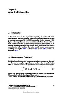
This integral gives the area under the graph of f , with the area under the positive part counting as positive area, and the area under the negative part of f counting as negative area, see figure 11.5. Before we continue, we need to define a term which we will use repeatedly in our description of integration. Definition 11.24. Let a and b be two real numbers with a < b. A partition of [a, b] is a finite sequence {x i }ni=0 of increasing numbers in [a, b] with x 0 = a and x n = b, a = x 0 < x 1 < x 2 · · · < x n−1 < x n = b. The partition is said to be uniform if there is a fixed number h, called the step length, such that x i − x i −1 = h = (b − a)/n for i = 1, . . . , n. 249

The traditional definition of the integral is based on a numerical approximation to the area. We pick a partition {x i } of [a, b], and in each subinterval [x i −1 , x i ] we determine the maximum and minimum of f (for convenience we assume that these values exist), mi =

min

x∈[x i −1 ,x i ]

f (x),

Mi =

max

x∈[x i −1 ,x i ]

f (x),

for i = 1, 2, . . . , n. We use these values to compute the two sums I=

n X

m i (x i − x i −1 ),

I=

i =1

n X

M i (x i − x i −1 ).

i =1

To define the integral, we consider larger partitions and consider the limits of I and I as the distance between neighbouring x i s goes to zero. If those limits are the same, we say that f is integrable, and the integral is given by this limit. More precisely, Z b f (x) d x = sup I = inf I , I= a

where the sup and inf are taken over all partitions of the interval [a, b]. This process is illustrated in figure 11.6 where we see how the piecewise constant approximations become better when the rectangles become narrower. The above definition can be used as a numerical method for computing approximations to the integral. We choose to work with either maxima or minima, select a partition of [a, b] as in figure 11.6, and add together the areas of the rectangles. The problem with this technique is that it can be both difficult and time consuming to determine the maxima or minima, even on a computer. However, it can be shown that the integral has a very convenient property: If we choose a point t i in each interval [x i −1 , x i ], then the sum I˜ =

n X

f (t i )(x i − x i −1 )

i =1

will also converge to the integral when the distance between neighbouring x i s goes to zero. If we choose t i equal to x i −1 or x i , we have a simple numerical method for computing the integral. An even better choice is the more symmetric t i = (x i + x i −1 )/2 which leads to the approximation I≈

n X ¡ ¢ f (x i + x i −1 )/2 )(x i − x i −1 ).

(11.28)

i =1

This is the so-called midpoint method which we will study in the next section. 250

x12

x12

(a)

x32

x52

x72

x92

(b)

Figure 11.7. The midpoint rule with one subinterval (a) and five subintervals (b).

In general, we can derive numerical integration methods by splitting the interval [a, b] into small subintervals, approximate f by a polynomial on each subinterval, integrate this polynomial rather than f , and then add together the contributions from each subinterval. This is the strategy we will follow, and this works as long as f can be approximated well by polynomials on each subinterval.

11.7 The midpoint method for numerical integration We have already introduced the midpoint rule (11.28) for numerical integration. In our standard framework for numerical methods based on polynomial approximation, we can consider this as using a constant approximation to the function f on each subinterval. Note that in the following we will always assume the partition to be uniform. Algorithm 11.25. Let f a function which is integrable on the interval [a, b] and let {x i }ni=0 be a uniform partition of [a, b]. In the midpoint rule, the integral of f is approximated by Z

b a

f (x) d x ≈ I mi d (h) = h

n X

f (x i −1/2 ),

(11.29)

i =1

where x i −1/2 = (x i + x i −1 )/2 = a + (i − 1/2)h. This may seem like a strangely formulated algorithm, but all there is to it is to compute the sum on the right in (11.29). The method is illustrated in figure 11.7 in the cases where we have one and five subintervals. 251

Example 11.26. Let us try the midpoint method on an example. As usual, it is wise to test on an example where we know the answer, so we can easily check the quality of the method. We choose the integral Z 1 cos x d x = sin 1 ≈ 0.8414709848 0

where the exact answer is easy to compute by traditional, symbolic methods. To test the method, we split the interval into 2k subintervals, for k = 1, 2, . . . , 10, i.e., we halve the step length each time. The result is h 0.500000 0.250000 0.125000 0.062500 0.031250 0.015625 0.007813 0.003906 0.001953 0.000977

I mi d (h) 0.85030065 0.84366632 0.84201907 0.84160796 0.84150523 0.84147954 0.84147312 0.84147152 0.84147112 0.84147102

Error −8.8 × 10-3 −2.2 × 10-3 −5.5 × 10-4 −1.4 × 10-4 −3.4 × 10-5 −8.6 × 10-6 −2.1 × 10-6 −5.3 × 10-7 −1.3 × 10-7 −3.3 × 10-8

By error, we here mean 1

Z 0

f (x) d x − I mi d (h).

Note that each time the step length is halved, the error seems to be reduced by a factor of 4. 11.7.1 Local error analysis As usual, we should try and keep track of the error. We first focus on what happens on one subinterval. In other words we want to study the error Z b ¡ ¢ f (x) d x − f a 1/2 (b − a), a 1/2 = (a + b)/2. (11.30) a

Once again, Taylor polynomials with remainders help us out. We expand both f (x) and f (a 1/2 ) about the the left endpoint (x − a)2 00 f (ξ1 ), 2 (a 1/2 − a)2 00 f (a 1/2 ) = f (a) + (a 1/2 − a) f 0 (a) + f (ξ2 ), 2 f (x) = f (a) + (x − a) f 0 (a) +

252

where ξ1 is a number in the interval (a, x) that depends on x, and ξ2 is in the interval (a, a 1/2 ). If we multiply the second Taylor expansion by (b−a), we obtain f (a 1/2 )(b − a) = f (a)(b − a) +

(b − a)3 00 (b − a)2 0 f (a) + f (ξ2 ). 2 8

Next, we integrate the Taylor expansion and obtain Z b Z b³ ´ (x − a)2 00 f (x) d x = f (a) + (x − a) f 0 (a) + f (ξ1 ) d x 2 a a Z £ ¤ 1 b 1 b = f (a)(b − a) + (x − a)2 a f 0 (a) + (x − a)2 f 00 (ξ1 ) d x 2 2 a Z 1 b (b − a)2 0 = f (a)(b − a) + f (a) + (x − a)2 f 00 (ξ1 ) d x. 2 2 a

(11.31)

(11.32)

We then see that the error can be written ¯ ¯ Z b ¯Z b ¯ ¯ ¯1 ¯ ¯ (b − a)3 00 2 00 ¯ ¯ ¯ ¯ = f (x) d x − f (a )(b − a) (x − a) f (ξ ) d x − (ξ ) f 1/2 1 2 ¯ ¯2 ¯ ¯ 8 a a ¯ ¯Z b 3 ¯ (b − a) ¯ 00 ¯ 1¯ ¯ f (ξ2 )¯ . ≤ ¯¯ (x − a)2 f 00 (ξ1 ) d x ¯¯ + 2 a 8 (11.33) For the last term, we use our standard trick, ¯ ¯ ¯ 00 ¯ ¯ f (ξ2 )¯ ≤ M = max ¯ f 00 (x)¯ . x∈[a,b]

(11.34)

Note that since ξ2 ∈ (a, a 1/2 ), we could just have taken the maximum over the interval [a, a 1/2 ], but we will see later that it is more convenient to maximise over the whole interval [a, b]. The first term in (11.33) needs some massaging. Let us do the work first, and explain afterwords, ¯Z ¯ Z ¯ 1 b¯ ¯ 1 ¯¯ b 2 00 ¯ ¯(x − a)2 f 00 (ξ1 )¯ d x ≤ (x − a) f (ξ ) d x 1 ¯ ¯ 2 a 2 a Z ¯ ¯ 1 b = (x − a)2 ¯ f 00 (ξ1 )¯ d x 2 a Z M b (11.35) ≤ (x − a)2 d x 2 a ¤b M 1£ = (x − a)3 a 2 3 M = (b − a)3 . 6 253

The first inequality is valid because when we move the absolute value sign inside the integral sign, the function that we integrate becomes nonnegative everywhere. This means that in the areas where the integrand in the original expression is negative, everything is now positive, and hence the second integral is larger than the first. 2 Next there is an equality which is valid because ¯ 00 (x − ¯ a) is never negative. The next inequality follows because we replace ¯ f (ξ1 )¯ with its maximum on the interval [a, b]. The last step is just the evaluation of the integral of (x − a)2 . We have now simplified both terms on the right in (11.33), so we have ¯Z ¯ ¯ ¯

b a

¯ ¯ M ¡ ¢ M f (x) d x − f a 1/2 (b − a)¯¯ ≤ (b − a)3 + (b − a)3 . 6 8

The result is the following lemma. Lemma 11.27. Let f be a continuous function whose first two derivatives are continuous on the interval [a.b]. The the error in the midpoint method, with only one interval, is bounded by ¯Z ¯ ¯ ¯

b

¯ ¯ 7M ¡ ¢ f (x) d x − f a 1/2 (b − a)¯¯ ≤ (b − a)3 , 24 a ¯ ¯ where M = maxx∈[a,b] ¯ f 00 (x)¯ and a 1/2 = (a + b)/2.

The importance of this lemma lies in the factor (b−a)3 . This means that if we reduce the size of the interval to half its width, the error in the midpoint method will be reduced by a factor of 8. Perhaps you feel completely lost in the work that led up to lemma 11.27. The wise way to read something like this is to first focus on the general idea that was used: Consider the error (11.30) and replace both f (x) and f (a 1/2 ) by its quadratic Taylor polynomials with remainders. If we do this, a number of terms cancel out and we are left with (11.33). At this point we use some standard techniques that give us the final inequality. Once you have an overview of the derivation, you should check that the details are correct and make sure you understand each step. 11.7.2 Global error analysis Above, we analysed the error on one subinterval. Now we want to see what happens when we add together the contributions from many subintervals; it should not surprise us that this may affect the error. 254

We consider the general case where we have a partition that divides [a, b] into n subintervals, each of width h. On each subinterval we use the simple midpoint rule that we analysed in the previous section, Z b n Z xi n X X f (x i −1/2 )h. I= f (x) d x = f (x) d x ≈ a

i =1 x i −1

i =1

The total error is then I − I mi d =

n µZ X i =1

xi

¶

x i −1

f (x) d x − f (x i −1/2 )h .

But the expression inside the parenthesis is just the local error on the interval [x i −1 , x i ]. We therefore have ¯ µZ ¶¯¯ ¯X n xi ¯ ¯ |I − I mi d | = ¯ f (x) d x − f (x i −1/2 )h ¯ ¯ ¯i =1 xi −1 ¯ ¯ Z n ¯ xi X ¯ ¯ ≤ f (x) d x − f (x i −1/2 )h ¯¯ ¯ ≤

i =1 x i −1 n 7h 3 X i =1

24

Mi

(11.36)

¯ ¯ where M i is the maximum of ¯ f 00 (x)¯ on the interval [x i −1 , x i ]. To simiplify the expression (11.36), we extend the maximum on [x i −1 , x i ] to all of [a, b]. This will usually make the maximum larger, so for all i we have ¯ ¯ ¯ ¯ M i = max ¯ f 00 (x)¯ ≤ max ¯ f 00 (x)¯ = M . x∈[x i −1 ,x i ]

x∈[a,b]

Now we can simplify (11.36) further, n 7h 3 n 7h 3 X X 7h 3 Mi ≤ M= nM . 24 i =1 24 i =1 24

(11.37)

Here, we need one final little observation. Recall that h = (b−a)/n, so hn = b−a. If we insert this in (11.37), we obtain our main result. Theorem 11.28. Suppose that f and its first two derivatives are continuous on the interval [a, b], and that the integral of f on [a, b] is approximated by the midpoint rule with n subintervals of equal width, Z

I=

b a

f (x) d x ≈ I mi d =

n X i =1

255

f (x i −1/2 )h.

Then the error is bounded by |I − I mi d | ≤ (b − a)

¯ ¯ 7h 2 max ¯ f 00 (x)¯ 24 x∈[a,b]

(11.38)

where x i −1/2 = a + (i − 1/2)h. This confirms the error behaviour that we saw in example 11.26: If h is reduced by a factor of 2, the error is reduced by a factor of 22 = 4. One notable omission in our discussion of the midpoint method is round-off error, which was a major concern in our study of numerical differentiation. The good news is that round-off error is not usually a problem in numerical integration. The only situation where round-off may cause problems is when the value of the integral is 0. In such a situation we may potentially add many numbers that sum to 0, and this may lead to cancellation effects. However, this is so rare that we will not discuss it here. You should be aware of the fact that the error estimate (11.38) is not the best possible in that the constant 7/24 can be reduced to 1/24, but then the derivation becomes much more complicated. 11.7.3 Estimating the step length The error estimate (11.38) lets us play a standard game: If someone demands that we compute an integral with error smaller than ², we can find a step length h that guarantees that we meet this demand. To make sure that the error is smaller than ², we enforce the inequality (b − a)

¯ ¯ 7h 2 max ¯ f 00 (x)¯ ≤ ² 24 x∈[a,b]

which we can easily solve for h, s 24² , h≤ 7(b − a)M

¯ ¯ M = max ¯ f 00 (x)¯ . x∈[a,b]

This is not quite as simple as it may look since we will have to estimate M , the maximum value of the second derivative. This can be difficult, but in some cases it is certainly possible, see exercise 4. 11.7.4 A detailed algorithm Algorithm 11.25 describes the midpoint method, but lacks a lot of detail. In this section we give a more detailed algorithm. 256

Whenever we compute a quantity numerically, we should try and estimate the error, otherwise we have no idea of the quality of our computation. A standard way to do this for numerical integration is to compute the integral for decreasing step lengths, and stop the computations when difference between two successive approximations is less than the tolerance. More precisely, we choose an initial step length h 0 and compute the approximations I mi d (h 0 ), I mi d (h 1 ), . . . , I mi d (h k ), . . . , where h k = h 0 /2k . Suppose I mi d (h k ) is our latest approximation. Then we estimate the relative error by the number |I mi d (h k ) − I mi d (h k−1 | |I mi d (h k )| and stop the computations if this is smaller than ². To avoid potential division by zero, we use the test |I mi d (h k ) − I mi d (h k−1 )| ≤ ²|I mi d (h k )|. As always, we should also limit the number of approximations that are computed. Algorithm 11.29. Suppose the function f , the interval [a, b], the length n 0 of the intitial partition, a positive tolerance ² < 1, and the maximum number of iterations M are given. The following algorithm will compute a sequence of Rb approximations to a f (x) d x by the midpoint rule, until the estimated relative error is smaller than ², or the maximum number of computed approximations reach M . The final approximation is stored in I . n := n 0 ; h := (b − a)/n; I := 0; x := a + h/2; for k := 1, 2, . . . , n I := I + f (x); x := x + h; j := 1; I := h ∗ I ; abser r := |I |; while j < M and abser r > ² ∗ |I | j := j + 1; I p := I ;

257

x0

x1

x0

x1

(a)

x3

x2

x4

x5

(b)

Figure 11.8. The trapezoid rule with one subinterval (a) and five subintervals (b).

n := 2n; h := (b − a)/n; I := 0; x := a + h/2; for k := 1, 2, . . . , n I := I + f (x); x := x + h; I := h ∗ I ; abser r := |I − I p|;

Note that we compute the first approximation outside the main loop. This is necessary in order to have meaningful estimates of the relative error (the first time we reach the top of the while loop we will always get past the condition). We store the previous approximation in I p so that we can estimate the error. In the coming sections we will describe two other methods for numerical integration. These can be implemented in algorithms similar to Algorithm 11.29. In fact, the only difference will be how the actual approximation to the integral is computed.

11.8 The trapezoid rule The midpoint method is based on a very simple polynomial approximation to the function f to be integrated on each subinterval; we simply use a constant approximation by interpolating the function value at the middle point. We are now going to consider a natural alternative; we approximate f on each subinterval with the secant that interpolates f at both ends of the subinterval. The situation is shown in figure 11.8a. The approximation to the integral is 258

the area of the trapezoidal figure under the secant so we have Z

b a

f (x) d x ≈

f (a) + f (b) (b − a). 2

(11.39)

To get good accuracy, we will have to split [a, b] into subintervals with a partition and use this approximation on each subinterval, see figure 11.8b. If we have a uniform partition {x i }ni=0 with step length h, we get the approximation Z

b a

f (x) d x =

n Z X

xi

i =1 x i −1

f (x) d x ≈

n f (x X i −1 ) + f (x i ) h. 2 i =1

(11.40)

We should always aim to make our computational methods as efficient as possible, and in this case an improvement is possible. Note that on the interval [x i −1 , x i ] we use the function values f (x i −1 ) and f (x i ), and on the next interval we use the values f (x i ) and f (x i +1 ). All function values, except the first and last, therefore occur twice in the sum on the right in (11.40). This means that if we implement this formula directly we do a lot of unnecessary work. From the explanation above the following observation follows.

Observation 11.30 (Trapezoid rule). Suppose we have a function f defined on an interval [a, b] and a partition {x i }ni=0 of [a.b]. If we approximate f by its secant on each subinterval and approximate the integral of f by the integral of the resulting piecewise linear approximation, we obtain the approximation Z

b a

¶ X f (a) + f (b) n−1 f (x) d x ≈ h + f (x i ) . 2 i =1 µ

(11.41)

In the formula (11.41) there are no redundant function evaluations. 11.8.1 Local error analysis Our next step is to analyse the error in the trapezoid method. We follow the same recipe as for the midpoint method and use Taylor series. Because of the similarities with the midpoint method, we will skip some of the details. We first study the error in the approximation (11.39) where we only have one secant. In this case the error is given by ¯Z ¯ ¯ ¯

b a

f (x) d x −

¯ ¯ f (a) + f (b) (b − a)¯¯ , 2

259

(11.42)

and the first step is to expand the function values f (x) and f (b) in Taylor series about a, (x − a)2 00 f (ξ1 ), 2 (b − a)2 00 f (b) = f (a) + (b − a) f 0 (a) + f (ξ2 ), 2 f (x) = f (a) + (x − a) f 0 (a) +

where ξ1 ∈ (a, x) and ξ2 ∈ (a, b). The integration of the Taylor series for f (x) we did in (11.32) so we just quote the result here, Z

b a

f (x) d x = f (a)(b − a) +

(b − a)2 0 1 f (a) + 2 2

Z

b a

(x − a)2 f 00 (ξ1 ) d x.

If we insert the Taylor series for f (b) we obtain (b − a)3 00 (b − a)2 0 f (a) + f (b) (b − a) = f (a)(b − a) + f (a) + f (ξ2 ). 2 2 4 If we insert these expressions into the error (11.42), the first two terms cancel against each other, and we obtain ¯Z ¯ ¯ ¯

b a

¯ ¯ Z b ¯ ¯ ¯1 ¯ f (a) + f (b) (b − a)3 00 2 00 ¯ ¯ f (x) d x − (x − a) f (ξ1 ) d x − (b − a)¯ ≤ ¯ f (ξ2 )¯¯ 2 2 a 4

These expressions can be simplified just like in (11.34) and (11.35), and this yields ¯Z b ¯ ¯ ¯ M f (a) + f (b) M ¯ f (x) d x − (b − a)¯¯ ≤ (b − a)3 + (b − a)3 . ¯ 2 6 4 a

Let us sum this up in a lemma. Lemma 11.31. Let f be a continuous function whose first two derivatives are continuous on the interval [a.b]. The the error in the trapezoid rule, with only one line segment on [a, b], is bounded by ¯Z ¯ ¯ ¯

b a

f (x) d x −

¯ ¯ 5M f (a) + f (b) (b − a)¯¯ ≤ (b − a)3 , 2 12

¯ ¯ where M = maxx∈[a,b] ¯ f 00 (x)¯.

This lemma is completely analogous to lemma 11.27 which describes the local error in the midpoint method. We particularly notice that even though the trapezoid rule uses two values of f , the error estimate is slightly larger than the 260

estimate for the midpoint method. The most important feature is the exponent on (b − a), which tells us how quickly the error goes to 0 when the interval width is reduced, and from this point of view the two methods are the same. In other words, we have gained nothing by approximating f by a linear functions instead of a constant. This does not mean that the trapezoid rule is bad, it rather means that the midpoint rule is unusually good. 11.8.2 Global error We can find an expression for the global error in the trapezoid rule in exactly the same way as we did for the midpoint rule, so we skip the proof. We sum everything up in a theorem about the trapezoid rule.

Theorem 11.32. Suppose that f and its first two derivatives are continuous on the interval [a, b], and that the integral of f on [a, b] is approximated by the trapezoid rule with n subintervals of equal width h, Z

I=

b a

¶ X f (a) + f (b) n−1 f (x) d x ≈ I t r ap = h f (x i ) . + 2 i =1 µ

Then the error is bounded by 2 ¯ ¯ ¯ ¯ ¯ I − I t r ap ¯ ≤ (b − a) 5h max ¯ f 00 (x)¯ . 12 x∈[a,b]

(11.43)

As we mentioned when we commented on the midpoint rule, the error estimates that we obtain are not best possible in the sense that it is possible to derive better error estimates (using other techniques) with smaller constants. In the case of the trapezoid rule, the constant can be reduced from 5/12 to 1/12. However, the fact remains that the trapezoid rule is a disappointing method compared to the midpoint rule.

11.9 Simpson’s rule The final method for numerical integration that we consider is Simpson’s rule. This method is based on approximating f by a parabola on each subinterval, which makes the derivation a bit more involved. The error analysis is essentially the same as before, but because the expressions are more complicated, it pays off to plan the analysis better. You may therefore find the material in this section more challenging than the treatment of the other two methods, and should 261

make sure that you have a good understanding of the error analysis for these methods before you start studying section 11.9.2. 11.9.1 Deriving Simpson’s rule As for the other methods, we derive Simpson’s rule in the simplest case where we use one parabola on all of [a, b]. We find the polynomial p 2 that interpolates f at a, a 1/2 = (a + b)/2 and b, and approximate the integral of f by the integral of p 2 . We could find p 2 via the Newton form, but in this case it is easier to use the Lagrange form. Another simiplification is to first contstruct Simpson’s rule in the case where a = −1, a 1/2 = 0, and b = 1, and then use this to generalise the method. The Lagrange form of the polyomial that interpolates f at −1, 0, 1, is given by x(x − 1) (x + 1)x p 2 (x) = f (−1) − f (0)(x + 1)(x − 1) + f (1) , 2 2 and it is easy to check that the interpolation conditions hold. To integrate p 2 , we must integrate each of the three polynomials in this expression. For the first one we have Z Z 1 1 1 1 2 1 h 1 3 1 2 i1 1 x(x − 1) d x = (x − x) d x = x − x = . −1 2 −1 2 −1 2 3 2 3 Similarly, we find 1

4 (x + 1)(x − 1) d x = , − 3 −1 Z

1 2

Z

1

1 (x + 1)x d x = . 3 −1

On the interval [−1, 1], Simpson’s rule therefore gives the approximation Z

1 −1

f (x) d x ≈

¢ 1¡ f (−1) + 4 f (0) + f (1) . 3

(11.44)

To obtain an approximation on the interval [a, b], we use a standard technique. Suppose that x and y are related by x = (b − a)

y +1 + a. 2

(11.45)

We see that if y varies in the interval [−1, 1], then x will vary in the interval [a, b]. We are going to use the relation (11.45) as a substitution in an integral, so we note that d x = (b − a)d y/2. We therefore have Z

b a

Z

f (x) d x =

1

µ

f −1

¶ Z b−a b−a 1 ˜ (y + 1) + a d y = f (y) d y, 2 2 −1

262

(11.46)

x0

x1

x2

x0

x1

(a)

x2

x3

x4

x5

x6

(b)

Figure 11.9. Simpson’s rule with one subinterval (a) and three subintervals (b).

where µ ¶ b−a f˜(y) = f (y + 1) + a . 2

To determine an approximaiton to the intgeral of f˜ on the interval [−1, 1], we can use Simpson’s rule (11.44). The result is Z

1

µ ¶ ³a +b ´ 1 ˜ 1 ˜ ˜ ˜ f (y) d y ≈ ( f (−1) + 4 f (0) + f (1)) = f (a) + 4 f + f (b) , 3 3 2 −1

since the relation in (11.45) maps −1 to a, the midpoint 0 to (a + b)/2, and the right endpoint b to 1. If we insert this in (11.46), we obtain Simpson’s rule for the general interval [a, b], see figure 11.9a. In practice, we will usually divide the interval [a, b] into smaller ntervals and use Simpson’s rule on each subinterval, see figure 11.9b.

Observation 11.33. Let f be an integrable function on the interval [a, b]. If f is interpolated by a quadratic polynomial p 2 at the points a, (a + b)/2 and b, then the integral of f can be approximated by the integral of p 2 , Z

b a

Z

f (x) d x ≈

b a

µ ¶ ³a +b ´ b−a p 2 (x) d x = f (a) + 4 f + f (b) . 6 2

(11.47)

We could just as well have derived this formula by doing the interpolation directly on the interval [a, b], but then the algebra becomes quite messy. 263

11.9.2 Local error analysis The next step is to analyse the error. We follow the usual recipe and perform Tay¡ ¢ lor expansions of f (x), f (a + b)/2 and f (b) around the left endpoint a. However, those Taylor expansions become long and tedious, so we are gong to see how we can predict what happens. For this, we define the error function, µ ¶ Z b ³a +b ´ b−a E(f ) = f (x) d x − f (a) + 4 f + f (b) . (11.48) 6 2 a Note that if f (x) is a polynomial of degree 2, then the interpolant p 2 will be exactly the same as f . Since the last term in (11.48) is the integral of p 2 , we see that the error E ( f ) will be 0 for any quadratic polynomial. We can check this by calculating the error for the three functions 1, x, and x 2 , b−a (1 + 4 + 1) = 0, 6 µ ¶ (b − a)(b + a) a +b 1 1 £ 2 ¤b b − a a +4 + b = (b 2 − a 2 ) − = 0, E (x) = x a − 2 6 2 2 2 µ ¶ 1 £ 3 ¤b b − a 2 (a + b)2 2 2 E (x ) = x a − a +4 +b 3 6 4 b−a 2 1 (a + ab + b 2 ) = (b 3 − a 3 ) − 3 3 ¢ 1¡ = b 3 − a 3 − (a 2 b + ab 2 + b 3 − a 3 − a 2 b − ab 2 ) 3 = 0. E (1) = (b − a) −

Let us also check what happens if f (x) = x 3 , µ ¶ (a + b)3 1 £ 4 ¤b b − a 3 3 3 a +4 +b E (x ) = x a − 4 6 8 µ ¶ 1¡ 4 b − a 3 a 3 + 3a 3 b + 3ab 2 + b 3 4 3 = b −a )− a + +b 4 6 2 ¢ 1 b −a 3¡ 3 = (b 4 − a 4 ) − × a + 3a 2 b + 3ab 2 + b 3 4 6 2 = 0. The fact that the error is zero when f (x) = x 3 comes as a pleasant surprise; by the construction of the method we can only expect the error to be 0 for quadratic polynomials. The above computations mean that ¡ ¢ E c 0 + c 1 x + c 2 x 2 + c 3 x 3 = c 0 E (1) + c 1 E (x) + c 2 E (x 2 ) + c 3 E (x 3 ) = 0 264

for any real numbers {c i }3i =0 , i.e., the error is 0 whenever f is a cubic polynomial. Lemma 11.34. Simpson’s rule is exact for cubic polynomials. To obtain an error estimate, suppose that f is a general function which can be expanded in a Taylor polynomial of degree 3 about a with remainder f (x) = T3 ( f ; x) + R 3 ( f ; x). Then we see that ¡ ¢ ¡ ¢ ¡ ¢ ¡ ¢ E ( f ) = E T3 ( f ) + R 3 ( f ) = E T3 ( f ) + E R 3 ( f ) = E R 3 ( f ) .

The second equality follows from simple properties of the integral and function evaluations, while the last equality follows because the error in Simpson’s rule is 0 for cubic polynomials. The Lagrange form of the error term is given by R 3 ( f ; x) =

(x − a)4 (i v) f (ξx ), 24

where ξx ∈ (a, x). We then find Z ¡ ¢ 1 b (x − a)4 f (i v) (ξx ) d x E R 3 ( f ; x) = 24 a µ ¶ b−a (b − a)4 (i v) (b − a)4 (i v) − 0+4 f (ξ(a+b)/2 ) + f (ξb ) 6 24 × 16 24 Z b 5¡ ¢ (b − a) 1 (x − a)4 f (i v) (ξx ) d x − = f (i v) (ξ(a+b)/2 ) + 4 f (i v) (ξb ) , 24 a 576 where ξ1 = ξ(a+b)/2 and ξ2 = ξb (the error is 0 at x = a). If we take absolute values, use the triangle inequality, the standard trick of replacing the function values by maxima over the whole interval [a, b], and evaluate the integral, we obtain |E ( f )| ≤

(b − a)5 (b − a)5 M+ (M + 4M ). 5 × 24 576

This gives the following estimate of the error. Lemma 11.35. If f is continuous and has continuous derivatives up to order 4 on the interval [a, b], the error in Simpson’s rule is bounded by |E ( f )| ≤

¯ ¯ 49 ¯ ¯ (b − a)5 max ¯ f (i v) (x)¯ . x∈[a,b] 2880

265

x0

x1

x2

x3

x4

x5

x6

Figure 11.10. Simpson’s rule with three subintervals.

We note that the error in Simpson’s rule depends on (b − a)5 , while the error in the midpoint rule and trapezoid rule depend on (b − a)3 . This means that the error in Simpson’s rule goes to zero much more quickly than for the other two methods when the width of the interval [a, b] is reduced. More precisely, a reduction of h by a factor of 2 will reduce the error by a factor of 32. As for the other two methods the constant 49/2880 is not best possible; it can be reduced to 1/2880 by using other techniques. 11.9.3 Composite Simpson’s rule Simpson’s rule is used just like the other numerical integration techniques we have studied: The interval over which f is to be integrated is split into subintervals, and Simpson’s rule is applied on neighbouring pairs of intervals, see figure 11.10. In other words, each parabola is defined over two subintervals which means that the total number of subintervals must be even and the number of given values of f must be odd. with x i = a + i h, Simpson’s rule on the interval If the partition is (x i )2n i =0 [x 2i −2 , x 2i ] is x 2i

Z

x 2i −2

f (x) d x ≈

¢ h¡ f (x 2i −2 + 4 f (x 2i −1 ) + f (x 2i ) . 3

The approximation to the total integral is therefore Z

b a

f (x) d x ≈

n ¡ ¢ hX ( f (x 2i −2 + 4 f (x 2i −1 ) + f (x 2i ) . 3 i =1

266

In this sum we observe that the right endpoint of one subinterval becomes the left endpoint of the following subinterval to the right. Therefore, if this is implemented directly, the function values at the points with an even subscript will be evaluated twice, except for the extreme endpoints a and b which only occur once in the sum. We can therefore rewrite the sum in a way that avoids these redundant evaluations. Observation 11.36. Suppose f is a function defined on the interval [a, b], and let {x i }2n be a uniform partition of [a, b] with step length h. The composite i =0 Simpson’s rule approximates the integral of f by Z

b a

f (x) d x ≈

¶ µ n n−1 X X h f (x 2i −1 ) . f (x 2i ) + 4 f (a) + f (b) + 2 3 i =1 i =1

With the midpoint rule, we computed a sequence of approximations to the integral by successively halving the width of the subintervals. The same is often done with Simpson’s rule, but then care should be taken to avoid unnecessary function evaluations since all the function values computed at one step will also be used at the next step, see exercise 7. 11.9.4 The error in the composite Simpson’s rule The approach we used to deduce the global error for the midpoint rule, can also be used for Simpson’s rule, see theorem 11.28. The following theorem sums this up. Theorem 11.37. Suppose that f and its first four derivatives are continuous on the interval [a, b], and that the integral of f on [a, b] is approximated by Simpson’s rule with 2n subintervals of equal width h. Then the error is bounded by ¯ ¯ 4 ¯ ¯ ¯E ( f )¯ ≤ (b − a) 49h max ¯¯ f (i v) (x)¯¯ . (11.49) 2880 x∈[a,b]

11.10 Summary In this chapter we have derived a three methods for numerical differentiation and three methods for numerical integration. All these methods and their error analyses may seem rather overwhelming, but they all follow a common thread: 267

Procedure 11.38. The following is a general procedure for deriving numerical methods for differentiation and integration: 1. Interpolate the function f by a polynomial p at suitable points. 2. Approximate the derivative or integral of f by the derivative or integral of p. This makes it possible to express the approximation in terms of function values of f . 3. Derive an estimate for the error by expanding the function values (other than the one at a) in Taylor series with remainders. 4D. For numerical differentiation, derive an estimate of the round-off error by assuming that the relative errors in the function values are bounded by ²∗ . By minimising the total error, an optimal step length h can be determined. 4I. For numerical integration, the global error can easily be derived from the local error using the technique leading up to theorem 11.28.

Perhaps the most delicate part of the above procedure is to choose the degree of the Taylor polynomials. This is discussed in exercise 6. It is procedure 11.38 that is the main content of this chapter. The individual methods are important in practice, but also serve as examples of how this procedure is implemented, and should show you how to derive other methods more suitable for your specific needs.

Exercises 11.1

a) Write a program that implements the numerical differentiation method f 0 (a) ≈

f (a + h) − f (a − h) , 2h

and test the method on the function f (x) = e x at a = 1. b) Determine the optimal value of h given in section 11.3.4 which minimises the total error. Use ²∗ = 7 × 10−17 . c) Use your program to determine the optimal value h of experimentally. d) Use the optimal value of h that you found in (c) to determine a better value for ²∗ in this specific example.

268

11.2 Repeat exercise 1, but compute the second derivative using the approximation f 00 (a) ≈

f (a + h) − 2 f (a) + f (a − h) h2

.

In (b) you should use the value of h given in observation 11.23. 11.3

a) Suppose that we want to derive a method for approximating the derivative of f at a which has the form f 0 (a) ≈ c 1 f (a − h) + c 2 f (a + h),

c 1 , c 2 ∈ R.

We want the method to be exact when f (x) = 1 and f (x) = x. Use these conditions to determine c 1 and c 2 . b) Show that the method in (a) is exact for all polynomials of degree 1, and compare it to the methods we have discussed in this chapter. c) Use the procedure in (a) and (b) to derive a method for approximating the second derivative of f , f 00 (a) ≈ c 1 f (a − h) + c 2 f (a) + c 3 f (a + h),

c 1 , c 2 , c 3 ∈ R,

by requiring that the method should be exact when f (x) = 1, x and x 2 . d) Show that the method in (c) is exact for all quadratic polynomials. 11.4

a) Write a program that implements the midpoint method as in algorithm 11.29 and test it on the integral Z 1 e x d x = e − 1. 0

b) Determine a value of h that guarantees that the absolute error is smaller than 10−10 . Run your program and check what the actual error is for this value of h. (You may have to adjust algorithm 11.29 slightly and print the absolute error.) 11.5 Repeat exercise 4, but use Simpson’s rule instead of the midpoint method. 11.6 It may sometimes be difficult to judge how many terms to include in the Taylor series used in the analysis of numerical methods. In this exercise we are going to see how this can be done. We use the numerical approximation f 0 (a) ≈

f (a + h) − f (a − h) 2h

in section 11.3 for our experiments. a) Do the same derivation as section 11.3.2, but include only two terms in the Taylor series (plus remainder). What happens? b) Do the same derivation as section 11.3.2, but include four terms in the Taylor series (plus remainder). What happens now? 11.7 When h is halved in the trapezoid method, some of the function values used with step length h/2 are the same as those used for step length h. Derive a formula for the trapezoid method with step length h/2 that makes use of the function values that were computed for step length h.

269