for Android and iPhone platform have been developed that are capable of detecting ... incidents of hacking into CCTV cameras at homes [77, 131], which can ...
Classification and Decision-Theoretic Framework for Detecting and Reporting Unseen Falls by
Shehroz Khan
A thesis presented to the University of Waterloo in fulfillment of the thesis requirement for the degree of Doctor of Philosophy in Computer Science
Waterloo, Ontario, Canada, 2016
c Shehroz Khan 2016
Declaration I hereby declare that I am the sole author of this thesis. This is a true copy of the thesis, including any required final revisions, as accepted by my examiners. I understand that my thesis may be made electronically available to the public.
ii
Abstract Detecting falls is critical for an activity recognition system to ensure the well being of an individual. However, falls occur rarely and infrequently, therefore sufficient data for them may not be available during training of the classifiers. Building a fall detection system in the absence of fall data is very challenging and can severely undermine the generalization capabilities of an activity recognition system. In this thesis, we present ideas from both classification and decision theory perspectives to handle scenarios when the training data for falls is not available. In traditional decision theoretic approaches, the utilities (or conversely costs) to report/not-report a fall or a non-fall are treated equally or the costs are deduced from the datasets, both of which are flawed. However, these costs are either difficult to compute or only available from domain experts. Therefore, in a typical fall detection system, we neither have a good model for falls nor an accurate estimate of utilities. In this thesis, we make contributions to handle both of these situations. In recent years, Hidden Markov Models (HMMs) have been used to model temporal dynamics of human activities. HMMs are generally built for normal activities and a threshold based on the log-likelihood of the training data is used to identify unseen falls. We show that such formulation to identify unseen fall activities is ill-posed for this problem. We present a new approach for the identification of falls using wearable devices in the absence of their training data but with plentiful data for normal Activities of Daily Living (ADL). We propose three ‘X-Factor’ Hidden Markov Model (XHMMs) approaches, which are similar to the traditional HMMs but have “inflated” output covariances (observation models). To estimate the inflated covariances, we propose a novel cross validation method to remove “outliers” or deviant sequences from the ADL that serves as proxies for the unseen falls and allow learning the XHMMs using only normal activities. We tested the proposed XHMM approaches on three activity recognition datasets and show high detection rates for unseen falls. We also show that supervised classification methods perform poorly when very limited fall data is available during the training phase. We present a novel decision theoretic approach to Fall detection (dtFall ) that aims to tackle the core problem when the model for falls and information about the costs/utilities associated with them is unavailable. We theoretically show that the expected regret will always be positive using dtFall instead of a maximum likelihood classifier. We present a new method to parameterize unseen falls such that training situations with no fall data can be handled. We also identify problems with theoretical thresholding to identify falls using decision theoretic modelling when training data for fall data is absent, and present an empirical thresholding technique to handle imperfect models for falls and non-falls. We also develop a new cost model based on severity of falls to provide an operational range iii
of utilities. We present results on three activity recognition datasets, and show how the results may generalize to the difficult problem of fall detection in the real world. Under the condition when falls occur sporadically and rarely in the test set, the results show that (a) knowing the difference in the cost between a reported fall and a false alarm is useful, (b) as the cost of false alarm gets bigger this becomes more significant, and (c) the difference in the cost of between a reported and non-reported fall is not that useful.
iv
Acknowledgements For the last 5 years, this PhD journey has been very special to me in terms of acquiring knowledge and becoming a better researcher. I am highly indebted to many people including my mentors, family members, colleagues and friends, without whom I would not have been able to complete this thesis. First and foremost, I would like to thank my supervisor Dr. Jesse Hoey for his guidance and support. He has been incredibly helpful in providing continuous feedback to improve upon my work. He patiently advised and mentored me throughout my graduate studies. I owe a lot to him in terms of skills, knowledge and vision that I developed being under his supervision. He helped me on several occasions on a personal and financial level and I am extremely grateful to him for his kind gestures to keep me afloat during tough times. I would like to thank my research committee comprising of Dr. Pascal Poupart and Dr. Dana Kuli´c for their support and constructive advices in framing my research topic. I am also thankful to my internal-external examiner Dr. Joon Lee for his positive feedback on my thesis. I am very thankful to my external examiner Prof. Philip Morrow for his feedback and suggestions to improve the quality of my thesis. During my stay at Waterloo, I met many wonderful people who made my stay here worthwhile. I would like to thank Dr. Daniel Vogel for giving me the opportunity to collaborate on several research projects. I am thankful to department secretaries Helen Jardine, Wendy Rush, Mitzi Schnabel, Margaret Towell and Paula Zister for providing assistance in administrative matters with a smiling face. Many thanks to Suzanne Safayeni for being a great teaching instructor and making my life simpler as a teaching assistant. My graduate student life would not have been easy without the incredible help of Gordon Boerke from the Computer Science Computing Facility. I would like to extend my gratitude to my colleague, friend and mentor Dr. Amir Ahmad for his support and encouragement throughout my graduate studies. Special thanks to Joshua Jung, Han Zhao and Mazen Melibari for providing feedback to improve the quality of my thesis. I would also like to mention the names of my colleagues Michelle E. Karg, Marek Grzes, Aarti Malhotra, Abdullah Rashwan, Areej Alhothali, Hadi Hosseini, Arthur Carvalho and Haiyu Zhen for their willingness to share ideas and overall support all this time. I am very thankful to my wife, Lubna, whose love, perseverance and dedication motivated me to do better every day. She remained extremely positive throughout this time and encouraged me on low days. Without her love, support and care, I would not be able to finish my graduate studies so smoothly. v
I would like to express thanks to my family members for their patience and for standing by me. My brothers Humair, Zubair, Mohsin, cousin Azeem, brother-in-law Hani and friend Zaki have always been concerned with my progress and wished for my success. It is sad that my father did not live to see this day; however, I posthumously would like to thank him for all the sacrifices he made in his lifetime for me. Many thanks to my mother for patiently waiting for me to graduate and showering me with her blessings. Lastly, I would like to express thanks to all of those who gave me direct and indirect support to complete this work. (Shehroz Khan)
vi
Dedication Dedicated to my wife Lubna...
vii
Table of Contents Declaration
ii
Abstract
iii
Acknowledgements
v
Dedication
vii
List of Figures
xiii
List of Tables
xv
Acronyms
xvii
1 Introduction
1
1.1
Why is Detecting Falls Important? . . . . . . . . . . . . . . . . . . . . . .
2
1.2
Challenges and Issues . . . . . . . . . . . . . . . . . . . . . . . . . . . . . .
4
1.3
General Description of the Problem . . . . . . . . . . . . . . . . . . . . . .
7
1.3.1
Practical Issues . . . . . . . . . . . . . . . . . . . . . . . . . . . . .
8
1.4
Problem Identification . . . . . . . . . . . . . . . . . . . . . . . . . . . . .
10
1.5
Contributions . . . . . . . . . . . . . . . . . . . . . . . . . . . . . . . . . .
13
1.6
Thesis Structure . . . . . . . . . . . . . . . . . . . . . . . . . . . . . . . . .
15
1.7
Publications . . . . . . . . . . . . . . . . . . . . . . . . . . . . . . . . . . .
16
ix
2 Literature Review 2.1
17
Survey of Existing Literature Review on Fall Detection . . . . . . . . . . .
18
2.1.1
Analysis . . . . . . . . . . . . . . . . . . . . . . . . . . . . . . . . .
21
2.2
Taxonomy for Studying Fall Detection . . . . . . . . . . . . . . . . . . . .
22
2.3
Fall Detection . . . . . . . . . . . . . . . . . . . . . . . . . . . . . . . . . .
24
2.3.1
Sequential Classification . . . . . . . . . . . . . . . . . . . . . . . .
24
2.3.2
One-Class Classification . . . . . . . . . . . . . . . . . . . . . . . .
26
2.3.3
Semi-Supervised and Sampling Techniques . . . . . . . . . . . . . .
28
Fall as an Abnormal Activity . . . . . . . . . . . . . . . . . . . . . . . . .
29
2.4.1
Vision based . . . . . . . . . . . . . . . . . . . . . . . . . . . . . . .
29
2.4.2
Sensor Based . . . . . . . . . . . . . . . . . . . . . . . . . . . . . .
31
2.5
Cost Sensitive Classification and Decision Theory . . . . . . . . . . . . . .
33
2.6
Cost of Falls . . . . . . . . . . . . . . . . . . . . . . . . . . . . . . . . . . .
35
2.7
Proposed Improvements . . . . . . . . . . . . . . . . . . . . . . . . . . . .
36
2.4
3 Classification of Unseen Falls
39
3.1
Brief Introduction to HMM . . . . . . . . . . . . . . . . . . . . . . . . . .
40
3.2
Motivation to use HMM . . . . . . . . . . . . . . . . . . . . . . . . . . . .
44
3.3
Pose HMM . . . . . . . . . . . . . . . . . . . . . . . . . . . . . . . . . . .
46
3.3.1
Threshold Based - (HMM1) . . . . . . . . . . . . . . . . . . . . . .
46
3.3.2
XHMM1 . . . . . . . . . . . . . . . . . . . . . . . . . . . . . . . . .
47
Normal Pose HMM . . . . . . . . . . . . . . . . . . . . . . . . . . . . . . .
47
3.4.1
Threshold Based - (HMM2) . . . . . . . . . . . . . . . . . . . . . .
47
3.4.2
XHMM2 . . . . . . . . . . . . . . . . . . . . . . . . . . . . . . . . .
48
3.4.3
HM MN ormOut . . . . . . . . . . . . . . . . . . . . . . . . . . . . . .
49
3.4
3.5
Activity HMM
. . . . . . . . . . . . . . . . . . . . . . . . . . . . . . . . .
49
XHMM3 . . . . . . . . . . . . . . . . . . . . . . . . . . . . . . . . .
49
Threshold Selection and Proxy Outliers . . . . . . . . . . . . . . . . . . . .
50
3.5.1 3.6
x
3.7
3.8
3.9
Experimental Design . . . . . . . . . . . . . . . . . . . . . . . . . . . . . .
54
3.7.1
Datasets . . . . . . . . . . . . . . . . . . . . . . . . . . . . . . . . .
54
3.7.2
Data Pre-Processing . . . . . . . . . . . . . . . . . . . . . . . . . .
58
3.7.3
Feature Extraction . . . . . . . . . . . . . . . . . . . . . . . . . . .
59
3.7.4
HMM Modelling . . . . . . . . . . . . . . . . . . . . . . . . . . . .
60
3.7.5
Performance Evaluation and Metric . . . . . . . . . . . . . . . . . .
62
Results . . . . . . . . . . . . . . . . . . . . . . . . . . . . . . . . . . . . . .
64
3.8.1
Training without fall data . . . . . . . . . . . . . . . . . . . . . . .
65
3.8.2
Feature Selection . . . . . . . . . . . . . . . . . . . . . . . . . . . .
73
Conclusions and Discussion . . . . . . . . . . . . . . . . . . . . . . . . . .
79
4 Supervised Fall Detection
81
4.1
Training with sufficient fall data . . . . . . . . . . . . . . . . . . . . . . . .
82
4.2
Are outliers representative of proxy for falls? . . . . . . . . . . . . . . . . .
86
4.3
Training with few falls . . . . . . . . . . . . . . . . . . . . . . . . . . . . .
90
4.4
Is knowing a type of fall useful? . . . . . . . . . . . . . . . . . . . . . . . .
95
4.5
Discrimination among different types of falls . . . . . . . . . . . . . . . . .
97
4.6
Conclusions and Discussion . . . . . . . . . . . . . . . . . . . . . . . . . . 102
5 Decision-Theoretic Reporting of Unseen Falls
105
5.1
Decision Theory . . . . . . . . . . . . . . . . . . . . . . . . . . . . . . . . . 107
5.2
Decision-Theoretic Framework - dtFall . . . . . . . . . . . . . . . . . . . . 109 5.2.1
Formulation for Fall Detection . . . . . . . . . . . . . . . . . . . . . 109
5.2.2
Maximum Likelihood Decision Function . . . . . . . . . . . . . . . 111
5.2.3
Expected Utility Decision Function . . . . . . . . . . . . . . . . . . 111
5.3
Decision-making without training data for falls . . . . . . . . . . . . . . . . 113
5.4
Problems with Theoretical Threshold . . . . . . . . . . . . . . . . . . . . . 115 5.4.1
Regret . . . . . . . . . . . . . . . . . . . . . . . . . . . . . . . . . . 116 xi
5.4.2 5.5
Negative Regret . . . . . . . . . . . . . . . . . . . . . . . . . . . . . 117
Empirical Threshold . . . . . . . . . . . . . . . . . . . . . . . . . . . . . . 119 5.5.1
One-Class Classification Case . . . . . . . . . . . . . . . . . . . . . 122
5.6
Mixture of Gaussian X-factor model . . . . . . . . . . . . . . . . . . . . . . 124
5.7
Experimental Analysis . . . . . . . . . . . . . . . . . . . . . . . . . . . . . 126
5.8
5.7.1
Parameters Setting . . . . . . . . . . . . . . . . . . . . . . . . . . . 127
5.7.2
Theoretical Threshold . . . . . . . . . . . . . . . . . . . . . . . . . 127
5.7.3
Empirical Threshold . . . . . . . . . . . . . . . . . . . . . . . . . . 128
Cost Model . . . . . . . . . . . . . . . . . . . . . . . . . . . . . . . . . . . 133 5.8.1
5.9
Fall Severity . . . . . . . . . . . . . . . . . . . . . . . . . . . . . . . 134
Conclusions and Discussion . . . . . . . . . . . . . . . . . . . . . . . . . . 136
6 Summary and Future Work 6.1
139
Future Directions . . . . . . . . . . . . . . . . . . . . . . . . . . . . . . . . 142
References
145
APPENDICES
167
A Boundary Value Analysis
169
B Algorithm to Compute Empirical Threshold and Regret for OCC case using GMM 171 C Prospect Theory
173
C.1 Decision-theoretic Formulation for Fall Detection . . . . . . . . . . . . . . 174
xii
List of Figures 1.1
X-Factor approach in 1 dimension [150]. . . . . . . . . . . . . . . . . . . .
12
2.1
Taxonomy for the study of fall detection methods. . . . . . . . . . . . . . .
24
3.1
Log-Likelihoods – (a) before and (c) after outlier removal. (b) shows boxplot of the quartiles for this data and the outliers for w = 1.5 . . . . . . . .
53
3.2
Cross Validation Scheme . . . . . . . . . . . . . . . . . . . . . . . . . . . .
54
3.3
geometric mean (gmean) with error bars across all subjects for DLR, MF and COV datasets . . . . . . . . . . . . . . . . . . . . . . . . . . . . . . .
70
3.4
Mean values of the top 5 features for DLR dataset
. . . . . . . . . . . . .
74
3.5
Mean values of the top 5 features for MF dataset . . . . . . . . . . . . . .
75
3.6
Mean values of the top 5 features for COV dataset
76
4.1
Effect of varying the amount of fall data in supervised learning on DLR dataset. The best performing X-Factor approaches is shown on the y-axis corresponding to zero training data (compared with Table 3.5b, Section 3.8). 92
4.2
Effect of varying the amount of fall data in supervised learning on MF dataset. The best performing X-Factor approach is shown on the y-axis corresponding to zero training data (compared with Table 3.6b, Section 3.8). 93
4.3
Effect of varying the amount of fall data in supervised learning on COV dataset. The best performing X-Factor approaches is shown on the y-axis corresponding to zero training data (compared with Table 3.7b, Section 3.8). 94
5.1
Decision surface for EUT and ML classifier. . . . . . . . . . . . . . . . . . 112 xiii
. . . . . . . . . . . . .
5.2
Graphical representation of a fall detection. . . . . . . . . . . . . . . . . . 113
5.3
Posterior probabilities of falls for each observation in the test set. . . . . . 118
5.4
Typical total misclassification cost curves [167] . . . . . . . . . . . . . . . . 120
5.5
mTh algorithm for finding the empirical threshold for the EUT case.
5.6
Block Diagram of the mTh algorithm for the OCC case. . . . . . . . . . . 125
5.7
Regret between EUT and ML. Shaded regions show negative regret. . . . . 129
5.8
Comparison of Regret between EUT and ML for DLR dataset . . . . . . . 130
5.9
Comparison of Regret between EUT and ML for MF dataset . . . . . . . . 131
. . . 123
5.10 Comparison of Regret between EUT and ML for COV dataset . . . . . . . 132 C.1
. . . . . . . . . . . . . . . . . . . . . . . . . . . . . . . . . . . . . . . . . . 175
xiv
List of Tables 3.1
Summary of different fall detection methods . . . . . . . . . . . . . . . . .
51
3.2
Extracted Features. . . . . . . . . . . . . . . . . . . . . . . . . . . . . . . .
61
3.3
Confusion Matrix . . . . . . . . . . . . . . . . . . . . . . . . . . . . . . . .
64
3.4
Performance Metrics . . . . . . . . . . . . . . . . . . . . . . . . . . . . . .
64
3.5
Performance of Fall Detection methods for DLR dataset for 2, 4 and 8 states. For XHMM3 (#states=#labelled activities + 1 state for fall). . . . . . . .
66
Performance of Fall Detection methods for MF dataset for 2, 4 and 8 states. For XHMM3 (#states=#labelled activities + 1 state for fall). . . . . . . .
67
Performance of Fall Detection methods for COV dataset for 2, 4 and 8 states. For XHMM3 (#states=#labelled activities + 1 state for fall). . . . . . . .
68
3.8
K-Fold Cross-Validated Paired t-Test . . . . . . . . . . . . . . . . . . . . .
72
3.9
Top 10/20 ranked features . . . . . . . . . . . . . . . . . . . . . . . . . . .
77
3.10 Performance of Fall Detection methods on reduced features for DLR dataset (Compare with Tables 3.5b and 3.5d) . . . . . . . . . . . . . . . . . . . . .
77
3.11 Performance of Fall Detection methods on reduced features for MF dataset (Compare with Tables 3.6b and 3.6d) . . . . . . . . . . . . . . . . . . . . .
78
3.12 Performance of Fall Detection methods on reduced features for COV dataset (Compare with Tables 3.7b and 3.7d) . . . . . . . . . . . . . . . . . . . . .
78
3.6 3.7
4.1 4.2
Supervised Fall Detection with full training data for falls and all normal activities for DLR dataset (compared with Table 3.5). . . . . . . . . . . . .
84
Supervised Fall Detection with full training data for falls and all normal activities for MF dataset (compared Table 3.6). . . . . . . . . . . . . . . .
84
xv
4.3
Supervised Fall Detection with full training data for falls and all normal activities for COV dataset (compared with Table 3.7). . . . . . . . . . . . .
84
Supervised Fall Detection with full training data for falls and all non-fall activities for DLR dataset (compared with Table 3.5 and Table 4.1). . . . .
85
Supervised Fall Detection with full training data for falls and all non-fall activities for MF dataset (compared with Table 3.6 and Table 4.2). . . . .
85
Supervised Fall Detection with full training data for falls and all non-fall activities for COV dataset (compared with Table 3.7 and Table 4.3). . . . .
85
4.7
Relationship between ω and %age coverage . . . . . . . . . . . . . . . . . .
87
4.8
Confusion Matrix and Rf (i) for DLR dataset. The alphabetical labels and the activity correspondence is: A=Jumping, B=Running, C=Walking, D=Sitting, E=Standing, F=Lying, G=Falling. . . . . . . . . . . . . . . . .
88
Confusion Matrix and Rf (i) for MF dataset. The alphabetical labels and the activity correspondence is: A=Car-in, B=Car-out, C=Jogging, D=Jumping, E=Sitting, F=Standing, G=Stairs, H=Walking, I=Falling. . . . . . . . . .
89
4.10 Confusion Matrix and Rf (i) for COV dataset. The alphabetical labels and the activity correspondence is: A=Near Fall, B=Standing, C=Lying, D=Sitting, E=Walking, F=Crouching, G=Falling. . . . . . . . . . . . . . .
89
4.11 Supervised Fall Detection for MF dataset with full training data for a type of fall and tested on all types of falls (compared with Tables 4.2, 3.6b and 3.6d). . . . . . . . . . . . . . . . . . . . . . . . . . . . . . . . . . . . . . . .
98
4.12 Supervised Fall Detection for COV dataset with full training data for a type of fall and tested on all types of falls (compared with Tables 4.3, 3.7b and 3.7d ). . . . . . . . . . . . . . . . . . . . . . . . . . . . . . . . . . . . . . .
99
4.4 4.5 4.6
4.9
4.13 Recall and Precision for MF dataset using supervised algorithms for identifying different types of falls. . . . . . . . . . . . . . . . . . . . . . . . . . . 100 4.14 Recall and Precision for COV dataset using supervised algorithms for identifying different types of falls. . . . . . . . . . . . . . . . . . . . . . . . . . 101 5.1
Utility Table. . . . . . . . . . . . . . . . . . . . . . . . . . . . . . . . . . . 109
xvi
Acronyms ADL Activities of Daily Living. CDC The Centers for Disease Control and Prevention. EM Expectation Maximization. EUT Expected Utility Theory. gmean geometric mean. GMM Gaussian Mixture Model. HMM Hidden Markov Model. MEMS Micro-Electro-Mechanical System. ML Maximum Likelihood. OCC One-Class Classification. OSVM One-Class Support Vector Machine. PT Prospect Theory. RF Random Forest. SVM Support Vector Machine. XHMM X-Factor Hidden Markov Model.
xvii
Chapter 1 Introduction Activity Recognition [31] studies the actions, behaviours and goals of a subject and attempts to build systems to recognize them with an aim to provide some sort of assistance. Research in activity recognition has led to the successful realization of intelligent pervasive environments that can provide context, assistance, monitoring and analysis of a subject’s activities that are usually backed up by advanced machine learning and vision algorithms. Most of the research in activity recognition is either based on sensors [31] or computer vision [53]. A drawback with sensor-based methods is their intrusive nature; a person has to wear sensor-based gadgets all the time which may be uncomfortable to carry and may lead to refusal to wear them [162]. Vision-based system works well in an indoor setting; however, when a person leaves the premises, these systems cannot provide much help. Research in activity recognition using wearable or computer vision sensors is mostly centred around identifying normal Activities of Daily Living (ADL) such as walking, running, standing, cycling, etc. and applied to monitor a subject’s movements, assess physical fitness and provide feedback. Though this research is meaningful, there can be scenarios where detection of unusual events becomes important, challenging and relevant. Missing out such unusual activities can impose health and safety risks on an individual. Falling is the most common type of unusual activity and the most studied [127, 74]. In real life, most falls are caused by sudden loss of balance due to an unexpected slip or trip, or loss of stability during movements such as turning, bending, or rising [156]. A fall can be defined in many ways depending upon the perspective of a health practitioner, carer, computer scientist / analyst or the subject himself. Most studies use a combination of topographical, biomechanical and behavioural components to define a fall [62] and using different fall definitions can influence the results of the study. The WHO report [139] defines a fall as 1
Definition “Fall: inadvertently coming to rest on the ground, floor or other lower level, excluding intentional change in position to rest on furniture, wall or other objects” According to Prevention of Falls Network Europe’s definition [98], a fall is an unexpected event in which the participants come to rest on the ground, floor or lower level. A majority of activity recognition datasets that collect falls in controlled laboratory settings, may not glean falls in fully naturalistic settings i.e. inclusion of intention may be present in those datasets. This very fact makes these collected falls artificial and not true representatives of actual falls. This issue is further discussed in section 1.3.1 and highlighted in Chapters 3, 4 and 5. In the following sections, we discuss the reasons why detecting falls is important, the challenges associated with detecting falls, the general description of the fall detection problem and the associated practical issues. We then identify major research problems and present an outline of the contributions proposed in this thesis. The chapter concludes with a brief summary of the overall structure of the thesis along with a list of publications resulting so far from this research.
1.1
Why is Detecting Falls Important?
Falls are the major cause of both fatal and non-fatal injury among people and create a hindrance in living independently. According to the report by SMARTRISK [169], in Canada in 2004, falls constituted 25% of all the unintentional injuries besides transport injuries or suicides, resulting in 2225 deaths, 105, 565 hospitalizations and 883, 676 nonhospitalizations. The report also suggests that falls accounted for 50% of all injuries that resulted in hospitalization, and was the leading cause of permanent partial disability (47%) and total permanent disability (50%). Falls were the leading cause of overall injury costs in Canada in 2004, accounting for $6.2 billion or 31% of total costs besides other unintentional injuries. According to the WHO report [139], the frequency of falls increases with an increase in age and frailty i.e. older adults are more prone to falling than younger adults. Around 28 − 35% of people aged 65 and over fall each year and this increases to around 32 − 42% for those over 70 years of age. Older people living in nursing homes fall more often than those living in the community (around 30 − 50%) and 40% of them experience recurrent falls [139]. The reason is that most of the older adults living in the nursing homes are more frail and these facilities report fall incidences more accurately [159]. According to the Public Health Agency of Canada [136], older adults in Canada who were hospitalized due to a fall spent up to three weeks in the hospital, which is three 2
times more than the average hospital stay among other age groups. They also comment that half of falls leading to hospitalizations occurred at home and the number of deaths resulting from falls increased with each increase in age category. Falls can impact a person both economically and psychologically. The economic impact can be categorized as either a Direct or Indirect cost [139]. Direct costs comprise of the health care costs, insurance, medications, surgery, treatment, rehabilitation [22] or long term care, whereas indirect costs include the loss of a job or income and productivity losses. Experiencing a fall may lead to a fear of falling [74], which in turn can result in lack of mobility, less productivity and can increase the risk of a fall. Fear of falling is identified as a major negative consequence associated with decline in physical and mental performance, progressive loss of mental health-related quality of life, decreased social contact and less physical activities [161, 193]. Boyd and Steven [16] conducted a study on 1709 adults aged 65 or older and found that more than one-third of them were moderately or very afraid of falling. An important factor in fall detection is the time spent unattended laying (on the floor) after incurring a fall as it is a key factor in determining the severity of a fall. Older adults, especially due to weakness and frailty, are unable to recover or get up from a fall if living on their own. This could lead to several other complications such as loss of consciousness, syncope, hypothermia, dehydration, broncho-pneumonia, pressure sores and even death [158, 122, 39]. Studies show that more than 20% of patients who were hospitalized because of a fall had been laying on the ground for an hour or more, and even though they had no direct injury resulting from a fall, their rate of morbidity was very high within the next 6 months [122]. To handle the issues discussed above, there is an imminent need for the development of robust fall detection methods. Ideally speaking, a robust fall detector must accurately detect and report falls immediately; however, in practice it may generate false alarms and can fail to report some falls. Both of these errors have different repercussions. Reporting excessive false alarms may lead a fall detector to be perceived as useless or ineffective and can result in rejection of the device. Failing to identify and report a fall could have life threatening consequences, causing a loss of confidence in the device, or increase in fear of falling. Successful design and implementation of efficient fall detection devices are necessary to reduce the response time for fall related injuries. These devices can also be helpful in reducing the economic burden on public health care resulting from the treatment, rehabilitation and longer stay of the patients at nursing homes due to falls.
3
1.2
Challenges and Issues
Falls can lead to economic, physical, social and psychological complications among individuals, and affects the elderly population more severely. Therefore, there is an imminent need for the development of intelligent pervasive systems that can accurately monitor a person’s activities and detect falls effectively. These types of systems form a major component of the overall goal of Assistive Technology [105] to help individuals to live independently and better integrate with the community. Most of the studies on fall detection either use computer vision (cameras), ambient sensors or wearable devices to capture data and employ either thresholding or machine learning techniques [127, 74]. Computer vision-based fall detectors work better in indoor settings and are non-intrusive; however, multiple cameras may need to be fitted in a living compound that could raise privacy concerns and may lead to their rejection. Moreover, a camera-based fall detection system may not be effective when a person goes outdoors, beyond the field of vision or if the illumination changes significantly [135]. The advantage of wearable sensors is that they are cost-effective, easy to wear and operate, and work both indoors and outdoors. However, they can be considered invasive and intrusive. These sensors must be worn all the time, which can also lead to their rejection [162]. Modern smartphones are also equipped with built-in sensors (accelerometer, gyroscope and other ambient sensors) and are considered ubiquitous, as many people carry them without considering them an additional gadget. Fall detection solutions based on smartphones may be ineffective in indoor settings as many people don’t keep them in their pockets or do not attach it to their body when inside their homes. Ambient sensing devices mostly use pressure sensors to detect falls and are cost effective and less intrusive. However, they can be highly sensitive to their surroundings, and can generate a lot more false alarms and may be considered ineffective by both the carer and user [127]. The data from both wearable and ambient devices can not be visually verified by a researcher or carer if the subject under observation is out of sight or outside the laboratory or care environment, and it is very hard to obtain labelled data for falls from the subject himself (e.g. noting the time of the day when a fall occurred) . There exist several commercial products for detecting falls such as Philips Lifeline [145]), MobileHelp Fall ButtonTM [126], AlarmCare [4], Galaxy Fall Detection System [176], Visonic Fall Detector [191] and Brickhouse Alert [20]1 . Recently, several mobile applications for Android and iPhone platform have been developed that are capable of detecting falls such as iFall [172], Fade [50], Seizario [165], and CareBeacon [24]. Many of these products 1
A detailed description of several commercial fall detectors is presented in [140, 46]
4
or mobile applications use fixed thresholds to detect falls, may fail to identify different types of falls, can produce many false alarms and require manual intervention. Most of these products are wearable (on chest, neck, waist, or in the pocket), so there are discomfort and adaptability issues as well. Brownsell and Hawley [21] conducted a study to understand the feasibility of employing fall detectors among older adults (age group 60-74). Their research concludes that most of the users who wore fall detectors felt more confident, independent and considered that a fall detector improved their safety. This study provides evidence of the importance of using fall detection systems in positively impacting the lives of people (older adults in this case). Noury et al. [135] mention that there is no wide scale deployment of fall detection devices in daily geriatric practice, largely due to their inadequate operations, ergonomics, high incidence of false alarms and the social stigmatization of the frailty of the older person. However, when the concept of detecting falls is presented to older adults they find great potential in it to improve their security, safety and well-being at home [74]. Therefore, there is a clear gap between the real utility and actual usability of fall detectors. Igual et al. [74] and Habib et al. [58] present several challenges and issues for the design of fall detectors that could impede their wider usability and adaptability. Many of these challenges are inter-linked and are discussed below: • Robustness – Many fall detection algorithms achieve high precision and recall under controlled laboratory settings; however, when applied to real-world situations their performance deteriorates [135]. Many studies collect human motion data for a few hours of ADLs, which is not sufficient to represent the actual activities carried out in the real world. Additionally, it is very difficult to run long-term studies to monitor the activities of people due to logistics, time, money, effort and the discomfort of the person. A major focus of developing fall detection systems is to help older adults; however, in most of the studies, young healthy individuals perform activities in their place as it is difficult to involve seniors in those studies due to ethics and health problems [140]. • Usability – Wearable devices aimed at fall detection can be uncomfortable to attach to the waist, chest or neck all the time. Smartphones offer a viable alternative due to their ubiquitous and pervasive nature; however, people keep smartphones in different places, orientations and often do not even carry them. Bad ergonomics, including the size, shape and weight of the device, can also impact the usability of such devices. Other factors that can affect the usability of these devices include manual intervention, a lack of interaction of the device with the user and a requirement of high technical skills to operate them. 5
• Acceptance – Acceptance of fall detection devices for the senior population is a challenge because they may not be technology savvy or inclined to learn about it. A study by Kurniawan [97] shows that older people are passive users of mobile phones, frightened of the consequences of using new and unfamiliar technology and find it difficult to grasp the complex designs of user interfaces (such as menus). Igual et al. [75] also find that people with intellectual disability face difficulty in navigating through the complicated interfaces of smartphones. • Limitations of the devices – A major challenge for using smartphones or other wearable devices is their battery drain time, which can be more in a smartphone as it is generally loaded with other mobile applications that can consume energy faster. Smartphones were not originally designed for fall detection; therefore, issues related to their placement, orientation, sensing architecture, stability of sampling frequency of the accelerometer and gyroscope can be a bottleneck. The camera based devices have limitations in working outdoors and in different lighting conditions. • Privacy Issues – Wearable devices can continuously and discreetly collect personal information, which when combined with other information such as geographical location, are enable to infer private information [153]. Context-aware systems including computer vision (or cameras) based fall detection methods are more prone to privacy concerns. Employing one or multiple cameras in a home environment may make the person feel surveilled or monitored round the clock. There have been several incidents of hacking into CCTV cameras at homes [77, 131], which can discourage a prospective user from installing such systems. • Real and Simulated Falls – Most of the papers reviewed in several survey papers on fall detection [74, 58, 127] indicate that a majority of the researchers test their systems using data collected through simulated falls. Klenk et al. [92] perform an experiment with older and younger adults, who are asked to perform real and simulated falls, and find significant variations in the acceleration and maximum number of jerks between real and simulated falls. Kangas et al.[82] find that some characteristics of falls that are detectable in simulated falls are not detectable in real life falls. Huynh et al. [72] note that in their study young adults perform the ADLs for testing purposes instead of the elderly. Since they may not fully simulate the actual activities of seniors, such fall detection systems may require re-adjustments of classification thresholds to perform well for the elderly. Bagal`a et al. [11] compare thirteen existing fall detection algorithms, test them on real world fall data and observe that these algorithms perform better on simulated falls than real falls. The methods based on thresholding on acceleration signals perform worse because thresholds are mostly 6
calibrated on simulated falls and are not suitable for real falls. A fixed threshold may not be the optimal strategy compared to a subject-specific threshold; however, such thresholds are difficult to generalize. Furthermore, they note that real falls are fewer in number than normal ADLs and therefore traditional metrics to measure performance of such systems should be chosen with care.
1.3
General Description of the Problem
The role of a fall detection system is to identify falls and report them. Identification or classification of falls is primarily a supervised classification problem, whereas falls reporting is a decision-theoretic approach to report falls optimally using the probabilities and the utilities used for the system. When sufficient training data for both falls and non-falls is present, this can either be stated as: • Classification Problem: In this case, the main challenge is to train the model for both falls and non-falls and compute likelihoods, given a fall or non-fall class and the prior probabilities to compute the posteriors i.e. P r(f |o) ∝ P r(o|f )P r(f ) P r(f¯|o) ∝ P r(o|f¯)P r(f¯) where O is a random variable that represents the observations and o ∈ O is an observation, P r(f |o) and P r(f¯|o) are the posterior probabilities, P r(o|f ) and P r(o|f¯) are the likelihoods, and P r(f ) and P r(f¯) are the prior probabilities for falls and nonfalls. The likelihoods can be calculated using a Maximum Likelihood (ML) approach, and the prior probabilities for falls and non-falls are generally computed as the ratio of falls and non-falls to the total training data. Normally, a decision is taken to classify a test sample as a fall or a non-fall based on posterior probabilities or likelihoods. • Decision-Theoretic Problem: In this case, apart from the probabilities, subjective utilities of different states of the systems are also utilized. A decision to report or not-report an action as a fall is taken based on the value of the decision function that maximizes the expected utility for performing an action: V (r|o) = P r(f |o)U (T P ) + P r(f¯|o)U (F P ) V (¯ r|o) = P r(f |o)U (M A) + P r(f¯|o)U (T N ) 7
where V (r|o) and V (¯ r|o) are the value functions to report or not-report a fall given an observation o, U(.) is a utility function that defines the subjective utility of True Positives (T P ), False Positives (F P ), Missed Alarms (M A) and True Negatives (T N )2 . We can define a normalized utility function (as shown in Table 5.1) s.t. U (T P ) = p, U (F P ) = q, U (M A) = 0 and U (T N ) = 1. We can, then set V (r|o) = V (¯ r|o), to get a theoretical decision function P r(f¯)(1 − q) P r(o|f ) = P r(f )p P r(o|f¯) and substituting P r(f |o) = 1 − P r(f¯|o), we get a theoretical threshold as τ = P r(f |o) =
1 p 1 + 1−q
(1.1)
(1.2)
The theoretical threshold, τ , is used to report or not-report a test observation o as a fall or a non-fall. The theoretical threshold shown in Equation 1.2 guarantees optimal decision under uncertainty, given true models for both falls and non-falls. The research question that is being asked by a fall detection and fall reporting system is also different. While a fall detection approach seeks to answer ‘Is an activity a fall ?’, fall reporting seeks to answer ‘Is it good to report an activity as a fall ?’.
1.3.1
Practical Issues
We now discuss some of the practical issues that can severely undermine the performance of a fall detection method in both the classification and decision-theoretic formulation. Lack of Availability of fall data A fall is an unusual event; therefore, the rarity of falls leads to a lack of sufficient data for them for training the classifiers. More than one type of fall may also occur and their unexpectedness make it difficult to model them in advance. Yin et al. [199] mention that due to the scarcity of abnormal activities (e.g. falls), it is a challenging problem to design a detection system that can reduce both the false positives and false negatives. Collecting 2
In this thesis, we follow the convention of treating the falls class as the positive class and the normal activities as the negative class. More discussion about these utilities in presented in Chapter 5.
8
fall data can be cumbersome because it may require the person to actually undergo a real fall which may be harmful and unsafe. Alternatively, artificial fall data can be collected in controlled laboratory settings; however, that may not be the true representative of actual falls and can ‘include intention’, which contravenes the definition of a fall discussed in Section 1. Analyzing artificially induced fall data can be good from the perspective of understanding and developing insights into falls as an activity but it does not simplify the difficult problem of detecting falls. As the artificial falls do not represent actual falls, the classification models built with them are more likely to suffer from over-fitting on the artificial falls and may poorly generalize on actual falls. The approaches that exclusively collect fall data still suffer from their limited quantity and ethics clearances. In addition to very few or no labelled data, the diversity and types of falls further makes it difficult to model them efficiently. The Centers for Disease Control and Prevention (CDC), USA [56] suggests that on an average, nursing home residents incur 2.6 falls per person per year. If an experiment is to be set up to collect real falls and assuming an activity is monitored every second by a sensor, then we get around 31.55 million normal activities per year in comparison to only 2.6 falls. The data for real falls may collected by running long-term experiments in nursing homes or private dwelling using wearable sensors and/or video. The falls data generated from such experiments can be sufficient enough to train supervised classifiers; however it will still be skewed towards normal activities. Stone and Skubic [175] conducted a study to collect activities from 13 apartments that contains a combined nine years of continuous data. In total, they obtained 9 actual falls along with 454 artificial falls. This study was done in realistic settings and highlights the rarity of falls and the difficulty in obtaining sufficient data for falls. The order of the average number of actual falls obtained in this study is consistent with the CDC statistic of falls per person per year. This high skew in the training data for falls may result in learning imperfect models and it is difficult to develop generalizable classifiers to identify falls efficiently. Lack of Understanding of Utilities and Costs A typical fall detection system must correctly identify and report falls; however, it may report some false alarms and fail to report some falls. Correctly identifying falls is critical for ensuring the safety of an individual; missing to report a fall can be considered as the worst outcome of a fall detection system, but reporting too many false alarms is not a good outcome either. However, both of these errors must not be given the same cost because they both represent two different types of ‘worst’ outcomes with two different ‘magnitudes’. Even though reporting a fall correctly is considered the best outcome of a fall detection classifier there is still some associated cost because the person has actually fallen, which 9
can lead to a possible injury and its subsequent consequences; like emotional stress to the subject or family and money spent on the treatment. Most fall detection methods either give equal cost to both types of errors or attempt to find a cost matrix from the data itself (more discussion in Section 2.5). However, both ideas are flawed because neither these costs (or conversely utilities) are known well in advance nor easily understood. Additionally, the relationship between these various costs (or utilities) is not clear. Deducing costs from data is not a good idea because the costs should not be data-specific but rather domain-specific. However, these costs may either be unavailable, hard to compute or may come from a domain expert.
1.4
Problem Identification
We discussed in Section 1.3 that the classification or detection of a fall is the outcome of a ML classifier that takes one uncertain state of nature to make a decision, which may not be an optimal action to perform. Whereas reporting a fall uses decision theory such that different outcomes combine probability of every state with their subjective utilities and the outcome with maximum expected utility is guaranteed to be an optimal decision. However, a fall is an abnormal activity that occurs rarely, infrequently and in diverse ways; therefore, it is very difficult to collect sufficient training data for them [89]. In the absence of training data for falls, we are left with the following major challenges: 1. We don’t know exactly what a fall may look like, and 2. We don’t know exactly the costs incurred during and after a fall. Without sufficient training data for falls, we may not build a model for them. For such cases, P r(f¯|o) can be estimated but not P r(f |o); moreover, the prior probability for falls can not be directly estimated from the training data because it may not be available. Therefore, neither the traditional ML approach nor the decision-theoretic approach can be applied directly to classify or report falls that were not observed before. Now, we discuss two approaches that can be used to identify unseen falls: (i) Setting Threshold on the Likelihood of Normal Activities In traditional classification methods that treat a fall as an abnormal activity (i.e. no knowledge about the parameters of unseen falls), a model is trained and parameters learned from normal activities (θf¯) using an iterative method (such as Expectation 10
Maximization (EM)) by maximizing the likelihood (P r(O|f¯)) to obtain locally optimum parameters θf∗¯ s.t. θf∗¯ = argmax P r(O|θf¯)
(1.3)
θf¯
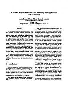
Given the parameters θf∗¯, the likelihood of each instance of the training set is computed and a threshold is calculated from them. This threshold is generally chosen as the maximum of negative of log-likelihood that shows the maximum deviation for the likelihood of an observation belonging to normal activities class. Any test observation that lies beyond this threshold can be classified as ‘not-normal’ or as a ‘fall’. However, this approach can only be used from the classification perspective to identify falls but not in the decision-theoretic sense to report falls because it does not provide probability estimates for falls and does not incorporate utilities. The value of such a threshold may be affected by the presence of spurious sensor readings or artifacts of the system. If a threshold is not set appropriately, then in the worst case, all falls may be classified as normal activities. To circumvent this problem, the threshold can be modified to be less sensitive to the noise in the sensor readings. That is, instead of setting the threshold as the maximum of negative of loglikelihood over the training set comprising of normal activities, the value of threshold is reduced. This modified threshold may reject some normal activities as ‘not-normal’ but it should be able to identify most of falls. (ii) Modelling Unseen Falls Instead of directly thresholding the log-likelihood computed from the training data containing normal activities, an alternative model for unseen falls can be built that can provide probability or likelihood estimates. The advantage of such a method is that it can be used both in the classification and decision-theoretic settings because it can provide probability estimates for both the classes. However, in the absence of training data for falls, this cannot be done directly. Quinn et al. [150] present a general framework to deal with unmodelled and unseen variations from the normal activities by proposing the ‘X-Factor approach’. In this method, the covariance of the normal dynamics is inflated to determine the regions with the highest likelihood that can be classified as ‘not-normal’. If the normal activities are assumed to follow a Gaussian distribution (or Gaussian Mixture Model (GMM)), then the parameters of the new distribution that represents ‘not-normal’ behaviour have the same mean as the normal activities model but different variance. The reason to vary only one parameter (i.e. variance or covariance) is to keep minimum assumptions about the 11
model for unseen falls. Figure 1.1 shows a 1-d Gaussian model for a normal activity class with zero mean and a corresponding X-factor that represents a ‘not-normal’ activity (or a fall class in our case) with the same mean but different variance. The data points that are at the extremes of the normal range are more likely to be classified as belonging to the X-factor (or falls) [150]. Therefore, using the X-Factor approach, the parameters of unseen falls can be estimated based on the parameters of normal activities. However, such a model may be imperfect and may not be expressive enough because it is an approximation for real falls.
0.4
non-fall X-factor
0.35
Pr(x|model)
0.3 0.25 0.2 0.15 0.1 0.05 0 -5
0
5
x
Figure 1.1: X-Factor approach in 1 dimension [150]. By modelling unseen falls using the X-Factor approach, we can estimate the likelihood for a test observation that can be used for their classification. This can be further extended to report falls by using decision theory by incorporating costs in a fall detection system. However, the costs occurring in a fall detection system are hard to compute and mostly unknown. Nonetheless, we would still like to build fall detection systems that are able to detect and report falls and are able to help people. The method to compute likelihood for unseen falls depends on the underlying approach. Below, we briefly present two approaches to estimate the likelihoods for unseen falls: 12
(a) Maximum Likelihood Approach: In this approach, we train a model and learn the parameters (θf¯) from the normal activities using ML, and use the X-Factor approach to compute the parameters for unseen falls (θf ). As discussed earlier, the parameters for both falls and non-falls only differ in their covariance. The scaling parameter for covariance can be found using cross-validation (see Chapter 3.6). The parameters θf can be used to compute the likelihood for unseen falls, P r(o|θf ), for the purpose of classification. (b) Bayesian Approach: In the Bayesian approach, we parameterize the model for unseen falls with θf , choose a prior distribution over it (P r(θf )) and integrate over all the possible values of θf to determine the expected likelihood for unseen falls, i.e.
E
Z
P r(θf ) [P r(o|f, θf )]
=
P r(o|f, θf )P r(θf ) θf
This expected likelihood for unseen falls can be combined with prior probabilities and costs to compute the expected value for reporting a fall. We present a particular case of using GMM with a specific prior and the X-factor approach within the decisiontheoretic framework to compute expected likelihood for unseen falls in Chapter 5. In this thesis, we identify these issues in developing a fall detection system and present methods that (i) Improve the traditional thresholding methods, and (ii) Build models for falls in the absence of their training data.
1.5
Contributions
Based on the above issues, this thesis presents contributions on the development of fall detection methods that treats a fall as an abnormal activity and builds classification and decision theoretic models using only the normal activities. These contributions are summarized below: 1. In recent years, Hidden Markov Model (HMM) have been applied to model human actions and activities [95]. Normally, HMMs are used to model the temporal dynamics of normal activities, then a threshold is placed to detect unseen falls [89]. The 13
maximum of negative of log-likelihood on the training data is generally used as a threshold to identify falls in the test set. In this thesis, we show that this approach of choosing a threshold is ill-suited for the problem of fall detection. We propose improvements by computing an improved threshold by rejecting spurious sensor data from the normal activities and are able to identify most falls correctly. We then propose three different types of X-Factor Hidden Markov Model (XHMM) that can learn alternative models for falls in the absence of their training data and need only sufficient normal activities data. The XHMMs are similar to HMMs with the exception that they have “inflated” output covariances in comparison to the models of the normal activities. To estimate the inflated covariances for the models of falls, we propose a novel cross-validation method that removes outliers from the observations of normal ADLs and uses them as a proxy for unseen falls, allowing the learning of XHMMs using only the data from the normal activities. These XHMMs are used to compute likelihoods for the unseen falls and help in their classification. In some cases, there may be few fall data to begin with; for such cases, we experimentally show that supervised classifiers perform poorly when the training data for falls is very limited in comparison to the XHMMs that require no training data for falls. 2. We present a decision theoretic framework for fall detection (dtFall ) based on Expected Utility Theory (EUT) that introduces a global utility function to encode our prior knowledge about falls and normal activities, and utilities of reporting/notreporting a fall/non-fall activity. We show that (a) the expected value of reporting/notreporting a fall using EUT will always be larger or same as ML, and (b) the ML method is a special case of EUT. We also present a method to estimate the expected likelihood for unseen falls by parameterizing falls and integrating out the effect of the parameter for falls by using a prior distribution. We derive an expression for the theoretical threshold to report unseen falls and show the problems associated with it in reporting falls optimally. These problems arise because the probabilistic models learned for non-falls and falls may not represent their true distributions and may not be expressive enough due to limited or unclean training data, or underlying assumptions and parameters of the algorithm. To tackle this issue, we modify an empirical thresholding algorithms that can deduce a probabilistic threshold from the training data to ensure that the EUT method performs better than the ML based approach. We also developed an exploratory cost model, which is based on the severity of falls, to estimate the parameters involved in deciding the utilities for a fall detection system.
14
1.6
Thesis Structure
In Chapter 2, we first survey the existing review papers on fall detection by presenting their major contributions and highlighting their limitations. Then we present a taxonomy for the study of fall detection based on the availability of fall data which is independent of the type of sensors used to capture human activities or the features extracted. We then present a comprehensive review of literature within each category identified by the proposed taxonomy. We conclude the chapter by proposing improvements in the existing research on fall detection. Chapter 3 begins with a brief discussion about traditional HMMs and discusses the proposed approaches that uses XHMMs and improved threshold based HMM approaches for detecting falls when their training data is not present. The chapter also discusses different datasets used in the thesis, mechanisms for extracting features and selecting relevant features. A novel cross-validation method is presented next, to remove outliers from the normal activities and treat them as proxies for unseen falls to help in estimating the parameters for the proposed XHMMs. We then show an experimental comparison between the traditional and improved threshold based HMM approaches and the XHMM methods and show the superior results of the proposed methods. Chapter 4 extends and compares the methods and results from Chapter 3 by considering supervised classification cases when some data for falls activity may be available for analysis. This chapter shows extensive experiments on situations when very few fall data are available, sufficient fall data are available or information on only one type of a fall is present that may be helpful for fall detection. In Chapter 5, we shift focus from classification to a decision-theoretic approach for fall reporting in the absence of training data for falls and the utilities of taking decisions to report or not-report falls and non-falls. This chapter builds upon the concepts of EUT to design a decision-theoretic framework (dtFall ) and shows its advantage over a ML classifier. We present a method to parameterize unseen falls to compute likelihood for unseen fall data using only the normal activities. We also provide a modification of a thresholding algorithm to adjust probability thresholds to take better decisions within the dtFall framework. The chapter further explores the concept of a new cost model that can be used in this framework to save cost in dollars. Results are shown for different activity recognition datasets and show the superiority of the proposed framework over a ML classifier. Chapter 6 draws significant conclusions from this thesis, identifies and proposes future research directions for possible extensions of this research work in a real-world setting.
15
1.7
Publications
The work in this thesis resulted in the following publications: 1. dtFall - Decision Theoretic Fall Detection for Unseen Falls, Shehroz S. Khan and Jesse Hoey, Submitted to 10th EAI International Conference on Pervasive Computing Technologies for Healthcare, 2016. 2. Detecting falls with X-Factor HMMs when the training data for falls is not available, Shehroz S. Khan, Michelle E. Karg, Dana Kulic and Jesse Hoey, Under Review in IEEE Journal of Biomedical and Health Informatics, 2015. 3. X-Factor HMMs for detecting falls in the absence of fall-specific training data, Shehroz S. Khan, Michelle E. Karg, Dana Kulic and Jesse Hoey, 6th International Workconference on Ambient Assisted Living (IWAAL 2014), Belfast, U.K., 2014. 4. Towards the Detection of Unusual Temporal Events during Activities Using HMMs, Shehroz S. Khan, Michelle E. Karg, Jesse Hoey and Dana Kulic, SAGAWARE: 2nd International Workshop on Situation, Activity and Goal Awareness, UbiComp, Pittsburgh, USA, 2012.
16
Chapter 2 Literature Review Detecting rare and abnormal human activities is a challenging task. The classification task becomes more difficult if their data is not present during the training phase or they did not occur earlier. Falling is one of the most notable abnormal activities that could result in life threatening consequences and partial or permanent disability. A fall is a short-term event and can occur in diverse ways, such as falls from walking or standing, falls from standing on supports, ladders, stairs, falls from sleeping or lying in the bed and falls from sitting on a chair [127]. However, falls from bed or a chair may last longer because the bed or chair may provide partial support to the falling person [203]. These different types of fall may bear similarities or can be significantly different from each other. A fall may also resemble some of the normal activities such as crouching, jumping [102, 130, 2], bending [113], sitting or lying down on the floor quickly [175] or suddenly stopping during running or walking [1]. As discussed in Chapter 1, a fall is a rare and infrequent activity and collecting data for falls is very difficult. Rigorous ethics clearances are required to set up experiments for fall detection and they can lead to injuries if proper precautions are not taken. To circumvent the issue of less availability of data for falls, researchers collect fall data either from seminaturalistic settings [128], from artificial falls in controlled laboratory settings[189], or from induced falls by applying external force [137, 124]. Artificial falls may not be a true representative of actual falls; however, they may provide important insights into the mechanism behind the real falls. In this chapter, we first survey the existing review papers on fall detection, present their contributions, highlight their limitations and draw a taxonomy for fall detection based on the availability of fall data. This taxonomy is independent of the type of sensors used to 17
capture human activities and specific type of feature extraction/selection methodologies. The taxonomy envisages the problem of fall detection from the point-of-view of learning models from human activities data by considering the problems associated in collecting falls data. We then present a comprehensive review of the current and significant research in the field of fall detection using the proposed taxonomy.
2.1
Survey of Existing Literature Review on Fall Detection
In the last decade, several review papers on fall detection have been published that discuss different aspects of fall detection problem involving various classification techniques and types of sensors. These review papers of existing research share several commonalities. In this section we survey major review papers on fall detection and highlight their focus of research, contributions and limitations. Noury et al. [135] report a short review on fall detection with an emphasis on the physics behind a fall, methods used to detect a fall and evaluation criteria based on statistical analysis. They discuss several analytical methods to detect falls by incorporating thresholds on the velocity of sensor readings, detecting no-movements, intense inversion of the polarity of the acceleration vector resulting from impact shock and suggest that such methods will result in high false positive rates. They mentioned since falls are rare, unsupervised machine learning techniques are likely to fail to identify the first fall event because it was not observed earlier. Supervised algorithms can only classify ‘known classes’ on which they are trained and such techniques may label a rare activity, like a fall, as ‘Others’ along with other activities e.g. to stumble, to slip etc. Yu [203] presents a survey on approaches and principles of fall detection for elderly patients. Yu first identifies the characteristics of falls from sleeping, sitting and standing and categorizes fall detection methods based on wearable, computer vision and ambient devices. These approaches were further broken down into specific techniques such as falls detection based on motion analysis, posture analysis, proximity analysis, inactivity detection, body shape and 3D head motion analysis and their merits and demerits discussed. Yu mentions that a fall is a rare event and it is important to develop techniques to deal with such scenarios. Yu further addresses the need for generic fall detection algorithms and fusion of different sensors such as wearable and vision sensors for providing better fall detection solutions. Perry et al. [144] present a survey on real-time fall detection methods based on techniques that measure only the acceleration, techniques that combine acceleration with other methods, and techniques that do not measure acceleration. They conclude that the methods measuring acceleration 18
are good at detecting falls. They also comment that placement of a sensor at the right position on the body can impact the accuracy of fall detection techniques. Hijaz et al. [68] present a survey on fall detection and monitoring ADL and categorize them into vision based, ambient-sensor based and kinematic-sensor based approaches. They identify kinematic-sensor based approaches that use accelerometer and/or gyroscopes as the best among them because of their cost effectiveness, portability, robustness and reliability. Mubashir et al. [127] present another survey on fall detection methods with an emphasis on different systems for fall detection and their underlying algorithms. They categorize fall detection approaches into three main categories: wearable device based, ambience device based and vision based. Within each category they review literature on approaches using accelerometer data, posture analysis, audio and video analysis, vibrational data, spatio-temporal analysis, change of shape or posture. They conclude that wearable and ambient devices are cheap and easy to install; however, vision based devices are more robust for detecting falls. Delahoz and Labrador [40] present a review of the state-of-the-art in fall detection and fall prevention systems along with qualitative comparisons among various studies. They categorize fall detection systems based on wearable devices and external sensors that includes vision based and ambient sensors. They also discuss general aspects of machine learning based fall detection systems such as feature extraction, feature construction and feature selection. They also summarize various classification algorithms such as Decision Trees, Naive Bayes, K-Nearest Neighbour and SVM; compare their time complexities and discuss strategies for model evaluation. They further discuss several design issues for fall detection and prevention systems including obtrusiveness, occlusion, multiple people in the scene, aging, privacy, computational costs, energy consumption, presence of noise, and defining appropriate thresholds. They also present a three-level taxonomy to describe the falling risks factors associated with a fall that includes physical, psychological and environmental factors and review several fall detection methods in terms of design issues and other parameters. Schwickert et al. [163] present a systematic review of fall detection techniques using wearable sensors. A major focus of their survey is to determine if the prior studies on fall detection use artificially recorded falls in a laboratory environment or natural falls in real-world circumstances, and find out that around 94% of studies use simulated falls. This is an important finding because it highlights the difficulty in obtaining real fall data due to their rarity. They also discuss that accelerometers along with other sensors such as gyroscopes, photo-diodes or barometric pressure sensors can help obtain better accuracy, and the placement of sensors on the body can be of importance in detecting falls. Zhang et al. [208] present a survey of research papers that exclusively use vision sensors, where they introduce several public datasets on fall detection and categorize vision based 19
techniques that uses single or multiple RGB cameras and 3D depth cameras. Pannurat et al. [140] present another review for automatic fall detection by categorizing the existing platforms based on either wearable and ambient devices, and the classification methods are divided into rule-based and machine learning techniques. They present a detailed overview of different aspects of fall detection, including sensor types and placement, subject details, ADLs and fall protocols, extracting features, classification methods, and performance evaluation. They also compare several fall detection products based on size, weight, sensor type, battery, transmission range and features and comment on future trends in the area of fall detection. Igual et al. [74] review 327 research papers on fall detection and categorize them as either context-aware systems or wearable devices (including smartphones). The context-aware systems are further categorized as based on cameras, floor sensors, infrared sensors, microphones and pressure sensors. They point out that despite the use of many feature extraction and machine learning techniques adopted by researchers, there is no standardized context-aware technique widely accepted by the research community in this field. The major contributions of their survey are the identification of emerging trends, ensuing challenges and outstanding issues in the field of fall detection. They point out that the limited availability of real life fall data is one of the significant issue which could hinder the system performance. Ward et al. [193] present a review of fall detection methods from the perspective of use and application of technology designed to detect falls and alert for help from end-user and health and social care staff. They categorize the technologies for fall detection based on manually operated devices, body worn automatic alarm systems and devices that detect changes which may increase the risk of falling. They also comment that the users of fall detection technologies are concerned with privacy, lack of human contact, user friendliness and appropriate training, but they identify the importance and benefits of such systems within the community. However, health and social care staff appear less informed and less convinced of the benefits of fall detection technologies. There are several other survey papers on fall detection [46, 65, 143, 171, 26, 96] that address similar ideas and issues already covered in the review papers discussed above. In the past few years, smart phones have becomes very popular as they are non-invasive, easy to carry, work both indoors and outdoors and are equipped with sensors that are useful for activity recognition. A recent comScore report [34] suggests that in the US up to 60% of people use smart phone devices as opposed to desktops and this number is close to or more than 50% in Canada and the UK. There has been a considerable amount of research work done for general activity recognition and fall detection using smartphones. Luque et al. [111] present a review of comparison and characterization of fall detection systems based on android smart phones. They mention that most of the techniques for fall detection based on smart phones either use machine learning (pattern matching) techniques or fixed 20
threshold(s). They conduct experiments with simulated falls, compare them with several algorithms and observe that the accuracy of the accelerometer based techniques to identify falls depends strongly on falls patterns1 . They also find difficulty in setting acceleration thresholds to get a good trade-off between false alarms and missed alarms. They further mention that the hardware limitations of the memory and real-time processing capabilities of the smart phones that may not support complex fall detection algorithms. Another major problem raised is the rate of battery consumption when mobile application for continuous monitoring are used. Casilari et al. [25] present another survey on analysis of android based smart phones solutions for fall detection. They systematically classify and compare many algorithms from the literature taking into account different criteria such as the system architecture, the employed sensors, the detection algorithms and the response in case of false alarms. Their study emphasizes the analysis of the evaluation methods that are employed to assess the effectiveness of the detection process.
2.1.1
Analysis
We observe several recurring themes that consistently appear among all the review papers we discussed previously: • There exists no standard methodology for fall detection in terms of type of sensors, feature engineering or machine learning techniques that supersedes other methods or perform consistently better than others. • It is noted in many of the above survey papers that techniques based on fixed thresholds on sensor readings, though simple to implement and computationally inexpensive, are very hard to generalize across different people and do not provide a good trade-off between false positive and false negatives [11, 74]. • Many of these survey papers reveal the complete lack of a reference framework, publicly available datasets and almost no access to real fall data to validate and compare to other methods. • Most of the above discussed survey papers review research on fall detection that assume sufficient data for falls and or adequate prior knowledge and understanding of falls. A fall is a rare event that can occur in diverse ways [39]; therefore, collecting 1
A fall pattern is characterized by a sudden decrease in acceleration and upon impact with the ground there is a sudden increase in the acceleration. This pattern is important to identify falls; however, different types of falls may lead to different values of accelerations.
21
sufficient fall data is very difficult. A long term experiment is required to glean real falls; however, such an experiment may only result in very few samples for real falls [175]. • Some of the review papers we discussed above acknowledge the rarity of real falls and the difficulty in generalizing results obtained from artificial or simulated falls; however, they did not review techniques that may be capable of identifying falls when their training data is very limited or not present. • Since most of the above discussed research papers assume sufficient falls collected from laboratories, we could not get useful insights about setting up long term experiments for collecting real falls data. By running long-term experiments, some data for real falls may be collected. However, recruiting the right target participants is a major challenge. Other challenges include ethics approvals and ensuring the safety of the participants. Since the data from these experiments will still be highly imbalanced, machine learning techniques that can handle this type of skewed data (such as cost-sensitive learning) needs to be studied and developed.
2.2
Taxonomy for Studying Fall Detection
Based on the inferences drawn from the recent review work on fall detection, we present a taxonomy for the study of fall detection methods that depends on the availability of training data for falls (see Figure 2.1). This taxonomy is independent of the type of sensors used to capture human motions and specific feature engineering methods employed to tackle this problem. The taxonomy has two high level categories: (I) and (II). The category (I) of the taxonomy shows the case when sufficient data for falls is available. In this category, due to the presence of sufficient falls and normal ADL data, different machine learning and heuristic based algorithms can be used such as threshold based, supervised classification and one-class classifiers (trained on sufficient fall data). However, in a real world scenario, this may not be the case as either we have too few fall data or none to begin with. Sometimes we may have few fall data along with a lot of unlabelled data. In these highly skewed data scenarios, heuristic and traditional supervised classification algorithms will not work and other classification frameworks based on One-Class Classification (OCC), outlier detection and cost-sensitive learning are needed; these techniques are mentioned in category (II) of the taxonomy. The approaches in category (I) attempt to detect the
22
actions of falling directly, whereas the approaches in category (II) instead try to detect unusual events or abnormal activities in general (as a fall is an abnormal activity). The techniques mentioned in category (I) that directly attempt to detect falls may use domain knowledge about the falling event [39] (e.g. sudden change in acceleration or its short duration) and use single/multiple threshold(s) to identify them. These methods also extract sophisticated features from the sensor readings and use supervised machine learning classifiers for identifying falls and normal activities. The techniques in category (II) that aim to detect falls as unusual events or abnormal activities rely on indirect evidence on the occurrence of falls [39]. This evidence may include prolonged inactivity, unusual locations, sudden change from normal behaviour and unknown or unseen behaviours. However, in these techniques the definition of “what is a normal behaviour?” needs to be defined carefully as it can vary for different people, especially for different age groups. These techniques only need to learn the normal behaviour; therefore, the inherent data imbalance between normal activities and falls is not an issue because they do not need samples for falls (or their different types) during training of the classifier. However, if the normal behaviour is not properly learned, these systems can result in large amount of false alarms because any slight variation from the normal behaviour would be classified as a fall. Finding an optimal threshold that can minimize both false alarms and missed alarms in these techniques is very challenging [199]. It is important to note that every abnormal behaviour or deviation from the normal behaviour does not imply the occurrence of a fall incident. As a result of these problems, such techniques require a lot of training data to effectively capture the normal behaviour or ‘normal concept’ over a long duration. The work presented in this thesis falls in the category (II)c, (II)d because we consider the case with no training data for falls and adopt either an outlier detection or OCC strategy (discussed in Chapter 3). For comparison purposes, we also show supervised fall detection method as shown in category (I)a in Chapter 4. Our work also use (II)a for imparting cost-sensitive classification and decision-theoretic reporting of fall; however we do not have training data for falls (discussed in Chapter 5). In the next sections, we review the literature based on the taxonomy for fall detection described above. We will not further discuss many supervised methods for fall detection and interested readers may find those references in the survey papers on fall detection discussed in the previous section. In our literature review, we present algorithms that work with different types of sensors, use a variety of machine learning algorithms, especially those that are known to model temporal, sequential and time series data and may work with a small amount of training data for falls or none at all. We also review prominent research done for unusual event / abnormal activity detection that may be well adapted for fall detection. 23
Taxonomy for the study of fall detection methods.
(I) Sufficient data for falls (a) If sufficient fall data is available, apply supervised machine learning techniques to identify normal activities along with falls [74]. (b) If sufficient fall data is available, apply threshold based techniques to detect falls from normal activities [15, 36]. (c) If sufficient fall data is available, apply OCC techniques to filter out normal activities [206, 201]. (II) Insufficient data for falls (a) If some fall data is available, apply cost sensitive classification algorithms or over/under-sampling techniques to identify normal activities along with falls [70, 175]. (b) If some fall data is available along with a lot of unlabelled data, apply semi-supervised techniques [104, 51]. (c) If sufficient fall data is not available or no fall data is available, apply outlier / anomaly / density based detection techniques to identify ‘unseen falls’ [88, 195]. (d) If sufficient fall data is not available or no fall data is available, apply OCC techniques to identify ‘unseen falls’ [90]. Figure 2.1: Taxonomy for the study of fall detection methods.
2.3 2.3.1
Fall Detection Sequential Classification
Several research works in fall detection are based on thresholding techniques [15, 36, 100, 29, 2, 99, 102, 100], wherein raw or processed sensor data is compared against a single 24
threshold or multiple pre-defined thresholds to detect a fall (see Taxonomy (I)b in Figure 2.1). The problem with thresholding techniques for fall detection is that it is very difficult to adapt thresholds to new or rare activities without prior knowledge. The ADL performed by people follow certain natural regularities and temporal smoothness [101], for example, people do not abruptly switch back and forth between walking and driving a car. The recent history of activities can help in predicting the present nature of activities. Lester et al. [101] show that using a sequence of posterior probabilities computed through static classifiers, and training HMM on them can significantly improve the performance and smoothness of the activity recognition system. In the past decade, there has been considerable research carried out in the field of activity recognition using HMM [101, 138, 95]. Most of his work is focused on modelling normal ADL using different types of sensors (such as accelerometers, GPS, WLAN, video cameras etc) and employing supervised learning for recognizing the activities. The data collected for detecting falls from different types of sensors is generally sequential in nature and HMMs are very well-suited for modelling sequential human motions with high accuracy [95]. These method based on HMM can be either used in a supervised manner or with fixed thresholds to detect falls (see Taxonomy (I)a and (I)b in Figure 2.1). Thome et al. [182] present a Hierarchical HMM (HHMM) approach for fall detection in video sequences. The HHMMs first layer has two states, an upright standing pose and lying. They study the relationship between angles in the 3D world and their projection onto the image plane and derive an error angle introduced by the image formation process for a standing posture. Based on this information, they differentiate other poses as ‘nonstanding’ and thus falls can be distinguished from other motions. A two-layer HMM approach, SensFall [110], is used to identify falls from other normal activities. In the first layer, the HMM classifies an unknown activity as normal vertical activity or “other”, while in the second stage the “other” activity is classified as either normal horizontal activity or as a fall. Hung et al. [71] present a two phase approach that uses an HMM and a SVM classifier in a home care sensory system for abnormal activity detection. The HMM is used to extract significant features from normal activity traces captured through RFID sensors. The features contain log-likelihood and time-stamp values, where a higher value of loglikelihood indicates normal activity and a lower value is abnormal. These feature vectors are then used to train a SVM classifier. Tokumitsu et al. [183] present an adaptive sensor network for home intrusion detection by human activity profiling. They use multiple HMMs for every subject in order to improve the detection accuracy and consider the fact that a single person can have multiple patterns for the same activity. The data is collected using infra-red sensors. A new sequence of activity is fed to all the HMMs and likelihoods are computed. If all the likelihoods calculated from corresponding HMMs are not greater than 25
pre-determined thresholds, then an anomaly is identified. They also present an empirical comparison of false-positive and miss-alarm rates, showing that both of them work against each other. Tong et al. [184] use the time series from human fall sequences collected using a triaxial accelerometer worn on upper body. An HMM is trained on events just before the collision for early fall prediction. They also compute two thresholds for fall prediction and detection to tune the accuracy. Shi et al. [168] use standard HMMs to model several normal activities including falls and perform classification with high accuracy from Micro-Electro-Mechanical System (MEMS) inertial sensors. Florentino-Lia˜ no et al. [54] present a hierarchical HMM based method to detect human activities including falls using a tri-axial accelerometer. Their method models both inter-activity and intra-activity dynamics and raw accelerometer signals were directly used to train the HMMs. No features were extracted in their method from the accelerometer signals; therefore the technique is sensitive to placement of the sensor on the subject’s body. Florentino-Lia˜ no et al. [55] extend this method by proposing a sensor position invariant measure on the raw accelerometer signal with the assumption that the sensor is placed in any fixed location within a region approximately bounded by a belt at the waist and a trouser pocket. The proposed method improved the precision and recall on falling and other normal activities. Cheng et al. [33] present a method to detect falls using surface electromyography and accelerometer signals. Histogram entropy is used to identify static and dynamic active segments. The later segments are further classified as dynamic gait activities and dynamic transition activities using angles calculated from the accelerometer. Finally, the dynamic transition activities were distinguished into normal dynamic activities and falls by using a threshold on accelerometer amplitude and dynamic gait activities were classified based on electromyography and accelerometer signals by using HMMs. Cheng et al. [32] present a fall detection algorithm based on pattern recognition and human posture analysis. The data is collected through a tri-axial accelerometer embedded in the smartphone and thirty temporal features are computed. The HMM is employed to filter out noisy character data and to perform dimensionality reduction. One-Class Support Vector Machine (OSVM) is applied to reduce false positives, followed by a posture analysis to counteract the missed alarms until a desired accuracy is achieved.
2.3.2
One-Class Classification
The techniques based on OCC attempt to build classification models on data from normal activities only, because the data for falls activity is either absent, or hard to collect (see Taxonomy (II)d in Figure 2.1). Alternatively, if sufficient falls are available, one-class 26
classifiers can be built on them to reject normal activities; however, in realistic settings such a strategy is highly unlikely because the availability of sufficient real fall data is difficult (see Taxonomy (I)c in Figure 2.1). Zhang et al. [206] train OSVM from positive samples (falls) and outliers from non-fall ADL and show that falls can be detected effectively. Yu et al. [201] propose to train Fuzzy OSVM on fall activity captured using video cameras and to tune parameters using fall and some non-fall activities. Their method assigns fuzzy membership to different training samples to reflect their importance during classification and is shown to perform better than OSVM. Yu et al. [200] introduce a video-based fall detection system for elderly people. They extract several video features and apply OCC techniques to determine whether the new instances lie in the ‘fall region’ or outside it to distinguish a fall from other activities such as walking, sitting, standing, crouching or lying. They test four OCC methods; k-center, k th nearest neighbour, OSVM and single class minimax probability machine (SCMPM) and find that SCMPM achieves the overall best performance among them. Han et al. [61] propose to use wireless signal propagation by employing the time variability and special diversity of Channel State Information as the indicator of human activities. Firstly a local outlier factor algorithm [18] is used to filter out dynamic activities such as walking, sitting, standing up and falling and then an OSVM is trained on fall activities to distinguish it from other normal activities. Zhou et al.[209] present a method to detect falls using transitions between the activities as a cue to model falls. They train supervised classification methods using normal activities, then extract transitions among these activities and use them to train an OSVM and show that it performs better than an OSVM trained with only normal activities. Yu et al. [202] present an online OSVM learning algorithm to detect falls captured through a single video source. They extract three types of features: ellipse, shape-structure and position features to build the normal model by an online OSVM which can be updated to new emerging postures. Additional rules were added to the system to report fewer false alarms and to improve fall detection performance. Popescu [146] presents a fall detection technique that uses acoustic signals of normal activities for training and detects fall sounds from it. They train OSVM, one-class nearest neighbour approach (OCNN) and One-class GMM (that uses a threshold) to train models on normal acoustic signals and find that OSVM performs the best. However, it is outperformed by its supervised counterpart. Khan et al. [87] propose an unsupervised acoustic fall detection system with interference suppression that makes use of the features extracted from the normal sound samples and construct an OSVM model to distinguish falls from non-falls. They show that in comparison to Popescu [146], their interference suppression technique makes a fall detection system less sensitive to interferences by using only two microphones. Medrano et al. [124] propose 27
to identify falls using a smartphone as a novelty from the normal activities and find that OCNN performs better than OSVM but is outperformed by supervised SVM. Taghvei and Kosuge [178] propose a method for a real-time visual state classification of a user with a walking support system. They extract visual features using principal component analysis and use an HMM for identifying real-time falls and state-recognition. In their experiment, an HMM is trained on walking activity and a threshold is separately calculated using a safe distance from the minimum probability distribution value of normal walking, which is adjusted with a constant. If the log-likelihood of a new activity is more than the calculated threshold, then it is identified as either a fall, sit or stand. A multi-class step is performed on top of the one-class classifier to identify one of the states of the HMM that corresponds to different activities including falls. A major drawback of this method is that the threshold is chosen only based on one activity (i.e. walking), but sitting and standing are also normal activities. Taghvaei et al. [177] present another fall detection method from a walker that uses features obtained from a depth camera and uses oneclass GMM to identify non-walking states and a continuous HMM for identifying different types of falls. The threshold for one-class GMM that represents normal activity is set experimentally. However, it is difficult to generalize this type of threshold across different people and there is no automatic way to tune it. Moreover, the threshold for a one-class GMM is only obtained using walking activity and it classifies sitting and falls as outlier activities. Rougier et al. [157] present a fall detection method using video feeds by tracking the person’s silhouette and performing shape analysis. They use GMM to distinguish falls from the normal data by manually setting a threshold on the log-likelihood.
2.3.3
Semi-Supervised and Sampling Techniques
In some cases, there may be few real falls available during the training phase (see Taxonomy (II)a and (II)b in Figure 2.1). To handle such a case, Stone and Skubic [175] present a two-stage fall detection system. In the first stage, a person’s vertical state is characterized in individual depth image frames followed by an ensemble of decision trees to compute a confidence on the occurrence of a fall. The data they collected has a fall ratio w.r.t. normal activities of 1 : 400. They under-sample the normal activities s.t. the ratio is reduced to 1 : 40 and create a decision tree ensemble. The activities studied in their analysis are standing, sitting, and lying down positions, near (within 4 m) versus far fall locations, and occluded versus not occluded fallers and report better results in comparison to the stateof-the-art methods. Debard et al. [39] use a weighted SVM to handle the imbalance in the dataset obtained for real world falls and normal activities from camera. The weights were computed using cross-validation and a grid search maximizing the area under the curve 28
of a Receiver Operating Characteristic (ROC) curve. Liu et al. [104] present a vision based semi-supervised learning mechanism for detecting falls and other ADL to overcome the exhaustive labelling of human activities. They use spatial field constraint energy to assist SVM-based activity decision with a Bayesian inference model, followed by a semisupervised step to retrain the classifier by automatically annotating the activities with the highest confidence. However, their method is sensitive to changes in environment, and needs to be retrained in new situations. Fahmi et al. [51] present a semi-supervised fall detection method using smartphones by first training a supervised algorithm using decision trees, then using fall profiles to develop a semi-supervised algorithm based on multiple thresholds. Medrano et al. [123] present a nearest neighbour based semi-supervised fall detection method for smartphones that can be personalized and updated easily as a new user records new ADL and the system is retrained on the fly. Makantasis et al. [113] present a 3D semi-supervised fall detection system that uses a monocular camera and uses an expert to refine an initially created small subset of labelled activity samples.
2.4
Fall as an Abnormal Activity
Due to the lack of availability of data for falls and the knowledge and understanding of what those falls might be, some researchers adopt an outlier detection approach. In these approaches, deviations from normal behaviour are flagged as an abnormal activity (see Taxonomy (II)c in Figure 2.1). Falling is one of the abnormal activities; therefore, such techniques can be adapted for fall detection. However, the concept of normal activities must be clearly defined because every abnormal activity may not be a fall. We review some of the abnormal activity recognition techniques that can be adapted for detecting falls.
2.4.1
Vision based
Several approaches have been proposed for abnormal activity recognition using the computer vision sensors. Xiang and Gong [195] propose a Dynamic Bayesian Network approach to model each normal video pattern and use a threshold to detect abnormal activity. This approach is simple; however, choosing a threshold remains challenging. Duong et al. [44] introduce the Switching Hidden Semi-Markov Model (SHSMM) for modelling normal activities and identifying abnormal activities using multiple camera tracking. However, they only focus on a specific type of abnormality that corresponds to spending too much or too
29
little time at a location and can be of interest in an elder care application. In a later extension work, Duong et al. [45] model the duration of activities using a Coxian distribution [132] and consider a hierarchy of activities to propose a SHSMM and show its application to activity segmentation and abnormality detection in smart environments. Zhang et al. [204] propose a semi-supervised adapted HMM framework for audio-visual data streams which comprises of supervised learning of normal data and unsupervised learning of unusual events using Bayesian adaptation. Their method has an iterative structure, where each iteration corresponds to a new detected unusual event. However, it is not clear from their work how many iterations are needed to terminate the process of outlier detection. Their model assumes that the normal activities data contains unusual events and guarantees one outlier per iteration. In cases where the normal activities data contains no unusual events, their method would still finds an outlier per iteration, which may be undesirable. Jiang et al. [80] mention that the HMM trained on small number of samples can overfit and propose a dynamic hierarchical clustering method based on a multi-sample based similarity measure. Their method starts with clustering the data in a few groups; the groups containing large numbers of samples are treated as normal patterns and HMMs are learned for each of them. This is followed by an iterative procedure of merging similar clusters (re-classifying) and re-training the remaining HMMs until no more merging occurs. An abnormal event is identified if its maximum log-likelihood from all normal events is below a threshold. They show their results on real surveillance video and point out that following the proposed method, the initial training and clustering errors due to overfitting will be sequentially corrected in later steps. However, the iterative re-classifying and re-training procedure can be computationally expensive as the size of the data grows. Pruteanu-Malinici and Carin [149] propose infinite HMM modelling to train normal video sequences; unusual events are detected if a low likelihood is observed. The infinite HMM modelling retains the full posterior density function as well as the underlying HMM states. Zhang et al. [207] propose an abnormal event detection algorithm from video sequences using a three-phased approach. First, they build a set of weak classifiers using Hierarchical Dirichlet Process Hidden Markov Model (HDP-HMM) and then use ensemble learning to identify abnormal events. Finally, they extract abnormal events from the normal ones in an unsupervised manner to reduce the false positive rates. Hu et al. [69] propose a refinement of the HDP-HMM method by incorporating Fisher Kernel into OSVM instead of ensemble learning and using sensor data instead of video data that can be discrete or continuous. The advantage of their method relies on using the HDP-HMM models that can decide on the appropriate number of states of the underlying HMM automatically. Antonakaki et al. [8] combine the use of HMM and OSVM to detect abnormal human behaviour using multiple cameras. They treat short term behaviour classification and trajectory classification 30
as separate classification problems by providing different set of features to both HMM and OSVM. Two feature vectors are computed per instance to capture short term behaviour and trajectory information and are fed to OSVM and HMM. Utilizing these two views of the data, they fuse the output of both the classifiers (logical OR) to identify abnormal activities. Matilainen et al. [119] present an unusual activity recognition method in noisy environments that uses a body part segmentation (BPS) algorithm [13], which gives an estimation of similarity between the current pose to the poses in the training data. The normal activities they considered are walking and sitting down and everything else is considered unusual activity. The BPS algorithm uses an HMM and a GMM which are trained through synthetic data created by motion capture. They use three sequences containing walking and falling over as the training set to find a statistically optimal threshold for unusual poses. They also propose to use a majority voting over large number of consecutive decisions for the actions that spans over a period of time and to mitigate the effect of single frames with incorrect decisions that helps in reducing false positive rates. However, the approach is based on carefully chosen optimal thresholds and training on a minimalist set of synthetic normal activities, which render this approach not very useful2 . Mahajan et al. [112] propose an activity recognition framework based on multi-layered finite state machines (FSM) built on top of a low level image processing module for spatio-temporal detection and limited object identification. The FSM learns the model for normal activities over a period of time in an unsupervised manner and can identify deviant activities as abnormal. Parisi and Wermter [141] propose a hierarchical Self Organizing Maps (SOM) based architecture for the detection of novel human behaviour in indoor environments by learning normal activities in an unsupervised manner using SOM and report novel behaviour as abnormal. To handle tracking errors, a first SOM is used to remove outliers from the training motion vectors. The pre-processed motion vectors are encoded by three types of descriptors – trajectories, body features and directions. A separate SOM is then trained for each type of descriptor. If a new observation deviates from the normal behaviour it is flagged as abnormal. Two threshold are empirically defined to remove outliers from the first SOM and detect abnormal behaviour from the other three SOMs.
2.4.2
Sensor Based
Many recent research papers focus on using sensor networks to detect abnormal activities. Yin et al. [199] propose a two-stage abnormal activity detection method in which an OSVM is first trained on normal activities and the abnormal activities are filtered out 2
A detailed review on several other types of video based abnormality detection methods is provided by Popoola and Wang [147]
31
and passed on to a kernel nonlinear regression routine to derive abnormal activity models from a general normal activity model in an unsupervised manner. The method iteratively detects different types of abnormal activities based on a threshold. They claim that this method provides a good trade-off between false alarms and abnormal activity detection without collecting and labelling the abnormal data. The data is collected by using wearable sensors attached to a user and abnormal instances were collected by simulating ‘falls’ and ‘slipping’ in different positions. Quinn et al. [150] present a general framework of Switched Linear Dynamical Systems (SLDS) for condition monitoring of a premature baby receiving intensive care. They introduce the ‘X-factor’ to deal with unmodelled variation from the normal events that may not have been seen previously. The general principle to identify an unusual event is to vary the covariance of the model of normal events to determine the interval with the highest likelihood where events can be classified as ‘not normal’. To model dynamic detection of abnormal events, they add a new factor to the existing SLDS model by inflating the system noise covariance of the normal dynamics. The sensor data is collected using various probes connected to each baby. The computation of the factor related to increasing the covariance remains challenging and is critical in this application. Cook et al. [35] present a method for activity discovery (AD) for smart-homes to identify behavioural patterns that do no belong to the pre-defined classes. Their algorithm scans the data and find the patterns that may represent similar activities and their variations. The algorithm then reports the best patterns that were found and the sensor event data can be compressed using the best pattern. The process is repeated several times until no new patterns can be found that compress the data. The search is carried out using Minimum Description Length principle [155] and final set of discovered patterns are clustered using quality threshold clustering method [67] in which the final number of clusters are not need to be specified apriori. This procedure can generate ‘Other’ or unknown activity cluster; however, it may contain some already discovered activities. The AD algorithm is performed on the ‘Other’ cluster and already discovered activities can be separated out from it, thereby reducing the ‘Other’ cluster size and the overall recognition of the system reportedly improved. Luca et al. [107] present a method for detecting rare hypermotor seizures in children by attaching accelerometer on the body. They use all the observed data to learn ‘normal behaviour’ and use extreme value theory to detect deviations from this model. Micucci et al. [125] evaluate fall detection methods that do not require fall data during training on different datasets collected using smartphone accelerometers. Their results show that in most of the cases, one-class K-nearest neighbour approach performs better or equivalent to the supervised SVM and KNN classification approaches that require data for both the normal and fall activities. The main contribution of this study is the finding that to design an effective fall detection method, prior understanding of falls patterns is not necessary.
32
2.5
Cost Sensitive Classification and Decision Theory
Learning from imbalanced data pertains to situations where data from one class is available in abundance, but the data from the other class is rare, difficult to collect or not readily available. Fall detection is a good example for imbalanced learning because the data for normal activities are easy to collect and sufficiently available in comparison to falls. Traditional supervised algorithms expect balanced datasets with equal misclassification costs for different classes. However, these algorithms fail to represent characteristics of the data and provide unfavourable accuracies when presented with imbalanced datasets [59], and their predictions may be dominated by the majority class [91]. The following are the general strategies adopted to handle learning from imbalanced datasets [59]: (i) Modify the training data distribution to correspond with the cost distribution of the classes by performing over-sampling or under-sampling. (ii) Applying Cost-sensitive classification techniques, (iii) Applying Kernel based methods, Active Learning, OCC and others. The main idea of cost-sensitive classification is to treat different costs in a classification problem differently. This can be done by either presenting a different cost matrix to a costinsensitive classifier or by changing the inner workings of a classification algorithm such that it uses a cost function to build a cost-sensitive classifier. Let us take the case of fall detection, where the dataset is mostly imbalanced in favour of normal activities. Identifying a rare activity (such as a fall) is important from the health and safety perspective, but the cost of a false alarm and a missed alarms should be very different and must not be treated equally. Therefore, when some data for falls is present for analysis along with abundant data for normal activities, techniques based on cost-sensitive classification can be used for fall detection (see Taxonomy (II)a in Figure 2.1). However, the incorporation of cost of classification while reporting or not-reporting a fall is absent in most of the studies on fall detection. It is important to note that the cost of errors in this problem should be domainspecific and not vary across different datasets. However, such costs are mostly unknown and hard to compute. Researchers use the following strategies to deal with cost-sensitive learning problems [91]: (i) Under/Over sampling of the majority/minority class to convert the original costsensitive problem into a traditional one (i.e., 0-1 loss)[27], 33
(ii) Changing the classification threshold [91, 167], and (iii) Using an ensemble of classifiers for estimating probabilities from different cost-sensitive classifiers and combine them for taking a decision [192, 118]. The objective of cost-sensitive learning is to minimize the overall cost of an action (for e.g. to report or not-report a fall) on the training data using a theoretical Bayes conditional risk. This problem can also be stated from a decision-theoretic perspective because costs and utilities are related concepts. Decision theory pertains to rational decision making by agents and can be employed to compute the expected cost of different actions in a classification problem, such as to report a fall or not. To compute the minimum expected cost, a Bayesian optimal probability threshold can be computed based on a given cost matrix. However, Elkan [48] recommends empirically computing a threshold to improve the accuracy of decision making rather than re-balancing the data to use a threshold of 0.5. Thai-Nghe et al. [181] present a method for cost-sensitive learning for imbalanced data that treats the cost-ratio of different errors as a hyper-parameter and optimize it locally to train the final models. Maloof [114] present a technique to deal with skewed datasets and unequal but unknown costs of error by performing ROC analysis to find the optimal operating threshold. However, the selection of an appropriate decision threshold is not automatic and it is unclear if this technique will work in the case of OCC, when the data for the negative class is absent. Huang et al. [70] perform cost-sensitive analysis for fall detection using Bayesian minimum risk and the Neyman-Pearson method. They vary the ratio of the cost of a missed alarm to a false alarm to find an optimal region of operation using the ROC curve. On the contrary, this ratio is generally fixed and must not depend on the dataset. The technique presented in the paper to estimate cost ratio can overfit the dataset without providing any intuitive interpretation about it. Traditional approaches for cost-sensitive learning for imbalanced datasets may not be directly applicable in the OCC problems. The reason is that in the OCC case, the data for one of the classes is absent during training; therefore, the probability estimates for the unseen or outlier class is hard to compute and estimating the costs of errors in such cases are even harder. Luo et al. [109] propose a cost-sensitive OSVM algorithm called Frequency based Support Vector Data Description (F-SVDD) and Write-Related SVDD (WR-SVDD) for intrusion detection problems. The SVDD method gives equal cost to classification errors, whereas F-SVDD gives higher cost to frequent short sequences occurring during system calls and WR-SVDD gives different costs to different system calls. Their experiments suggest that giving different costs to system users (than to processes) result in higher performance. Yaniv and Nisenson [47] consider OCC from a game-theoretic perspective as a game between the learner and an adversary, in which the target distribution 34
is known to the learner and its goal is to construct a classifier that can minimize false negative error for a given false positive error. They mention that low-density rejection is worst-case optimal if the learner uses hard decision strategies. This formulation is more relevant for the intrusion detection problem, where it is necessary to precisely quantify what an adversary can do or knows about the target distribution. If such an adversary exists, who knows all the parameters of the game including the learner’s strategy, it can completely demolish the learner that uses hard strategies. We argue that this framework is not suitable for fall detection problems because such an adversary does not exist in this problem. A fall detection problem is more about recognizing falls and taking the right decisions; therefore, a decision-theoretic framework is more apt to handle it. There is very sparse literature on decision-theoretic methods for identification of outliers or rare events/activities. Decision-theoretic approaches have been applied in some tasks, including detecting anomalies in internet paths [52], intrusion detection [115] and fault detection in wireless sensor networks [129]. Fida et al. [52] propose an algorithm to detect anomalies on an end-to-end internet path based on the likelihood ratio. The normal internet responses are modelled using a Gaussian distribution, whereas the anomalous activities are modelled with a different mean than normal. Based on user defined true positive and false positive rates they define thresholds to detect both hypotheses. Nandi et al. [129] define an overall risk function for fault detection on sensor networks and seek a Bayes test which minimizes the overall risk function in the critical region. Decisions are then made purely on the optimal Bayes test. Torgo and Lopes [185] present a utility based fraud detection method that produces a ranking that is ordered by decreasing expected utility of inspecting the candidate cases. Their general framework requires additional information such as historical data with information on past inspection activities, set of candidate cases for inspection and utility function to use. However, this framework may not be applicable to scenarios where outliers are not observed in the past.
2.6
Cost of Falls
Computing the costs incurred during and after a fall requires a long term study and it can vary across different countries, healthcare systems and the target age group. There are several research studies that attempt to calculate the cost of falls and false alarms. Heinrich et al. [66] review 32 studies on falls across different countries and found that the cost per fall ranged from $1, 059 to $10, 913. Newton et al. [133] present a study to quantify the immediate costs to the Ambulance Services (Newcastle, UK) of attending to fallers and found that 11% of them required assistance only and not hospitalization. 35
However, there is the cost of the ambulance and the time spent in assistance, which comes out to be £145.83 (≈ $231) per fall. This amount provides a very simple estimate on the cost of reporting a non-fall as a fall. However, there are many hidden costs that are not taken into account by this estimate. For example, an excess of false alarms may lead to a higher rate of technology rejection. This, in turn, would lead to a higher number of people living without fall detection systems, which eventually leads to a higher rate of unreported falls – that is highly undesirable and costly. Ikefuji et al. [76] articulate that “Catastrophic risks are important” but “The price to reduce catastrophic risk is finite”. Not-reporting a fall is catastrophic in the sense that it could lead to the loss of life of an individual. However, we could not find research on finding the cost of not-reporting a fall, primarily this is not an obvious question to researchers and its value is hard to estimate. The cost of unreported catastrophic events is difficult to model mostly due to unreliable or lack of data [17]; however, if such cost is ignored it can have adverse effects. Fred [17] suggests that epidemic data can be unreliable as there were many asymptotic or mild unreported cases in the H1N1 influenza pandemic of 2009. Xue et al. [197] use Susceptible-Exposed-Infected-Recovered model to estimate cost-benefit of school closure during influenza pandemic. Xue et al. [196] use quasi-Poisson regression model to estimate the impact of missing costs of unreported complications and sick leave arising from influenza. The data was available from health care services and sick leave certification and they estimated direct and indirect costs associated with the disease.
2.7
Proposed Improvements
Based on the taxonomy of the study of fall detection presented in Section 2.2, we can broadly divide the techniques to handle fall detection into those that assume sufficient data for falls and those with very few or no training data for falls. The former approaches rely on sufficient falls for training the supervised classifiers, which is hard to obtain in practice and is normally collected in a laboratory under non-naturalistic settings. This assumption has the disadvantage that the collected falls may not be a true representative of actual falls, and learning with a few contrived fall samples may not produce generalized classifiers that work for all people. The latter approaches assume a more realistic setting, where we may have insufficient or no training data for falls. These techniques attempt to learn a ‘normal concept’ from the labelled data, apply outlier detection techniques, and find a threshold to detect unseen falls. However, a major challenge in such techniques is to learn the ‘normal concept’ correctly and decide on a threshold that gives a good compromise of false-positives and false-negatives. The techniques that use OSVM suffer from choice of 36
appropriate kernel, kernel parameters and the parameter to set the soft margin. If the size of training data is large, then the optimization routine in OSVM can take a long time for convergence, especially if some data objects are exactly on top of each other and compete to become support vectors. The traditional techniques based on HMM choose the maximum of the negative of likelihood on the training data as a threshold to detect falls [88]. However, the data captured through sensors for fall detection contain artifacts due to spurious sensor readings, hardware noise or labelling errors. A threshold chosen on such data can be detrimental to the overall performance of a fall detection classifier and may result in accepting unseen falls as member of the normal class. Several researchers remove artifacts from the sensor data to improve the overall performance of fall detection classifiers [141, 32, 7]. The rejected outlier data is generally discarded and not used for further analysis. We hypothesize that such outlier data can help in setting the boundaries of the normal concept in a case when a fall is not observed before. Using these ideas, in Chapter 3, we present three new approaches for fall detection that use the traditional HMMs to learn the normal concept and do not need fall data during the training time. We then present a X-Factor approach to inflate the covariances of the learned model for normal activities and infer a model for falls. The hidden states of these three HMMs either model poses of a particular normal activity, poses for general normal activities or transition between each normal activity. To find an automatic threshold with a good balance for fall and normal activity detection, a novel cross-validation method is presented that rejects few outliers from the normal activities data to help estimating parameters of the X-Factor HMM models. In some situations few falls may be present or data from different types of falls may be available. In Chapter 4, we move forward to demonstrate the relationship between increasing the number of training data for falls and the performance of several supervised classifiers. We also perform experiments to understand the effect of knowing a type of fall in identifying other types of falls in a supervised classification setting. The methods that use threshold optimization for fall detection use the threshold as a slider between raising false alarms or risking missed alarms [183]. Choosing the threshold too low or high results in accepting all fall events as normal or rejecting most of the normal activities as falls. However, as stated earlier, the costs of false alarms and missed alarms are not the same for a fall detection application. Therefore, a decision-theoretic model is required that can minimize/maximize a cost/utility function instead of setting a threshold to take the rational decision to report or not-report a fall. The lack of methods to model a rare class and lack of understanding of the utilities/costs imposes a challenge to design decision-theoretic approaches for rare class classification. In Chapter 5 we present a decision-theoretic framework to classify unseen falls that addresses these issues in detail. 37
Chapter 3 Classification of Unseen Falls A lot of the current research on activity recognition is centred around the identification of the normal ADL [187, 30]. Identification of normal ADL, for e.g. walking, sleeping, hand washing, making breakfast etc., is important to understand a person’s behaviour, goals and actions [3] and forms the core of assistive technologies [105]. However, in certain situations, a more challenging, useful and interesting research problem is to identify cases when an abnormal activity occurs, as it can have direct implications on the health and safety of an individual. An important abnormal activity is the occurrence of a fall. However, falls occur rarely, infrequently and unexpectedly w.r.t. the other normal ADLs and this leads to either little or no training data for them [74] (more details in Chapters 1 and 2). This imbalance in the training data for falls and normal activities makes it difficult to develop generalizable supervised classifiers to identify falls. A typical supervised activity recognition system may misclassify ‘fall’ as one of the already existing normal activities, as ‘fall’ may not be included in the classifier training set. An alternative strategy is to build fall detection specific classifiers [36] that assume abundant training data for falls, which is hard to obtain in practice. Another challenge is the data collection for falls, as it may require a person to actually undergo falling which may be harmful, ethically questionable, and cumbersome and the falling incidences collected in controlled laboratory settings may not be the true representative of falls in naturalistic settings [82]. One of the research question we address in this thesis is: Can we recognise falls by observing only normal ADL with no training data for falls in a person independent manner?. We use Hidden Markov Models (HMMs) for the present task as they are very well-suited for sequential data and can model human motions with high accuracy [95] (see further discussion in Sections 3.1 and 3.2). As discussed in Chapter 2, there are two ways to detect falls using HMMs (see Taxonomy shown in Figure 2.1): (a) train an HMM involving 39
normal activities and falls and perform supervised classification, (b) train an HMM for normal activities and use a threshold to identify a fall as an outlier. The problem with the former approach is that sufficient fall data are required to train a model for falls, which is very difficult to obtain in the real world. In this chapter, we use an outlier detection approach to identify falls and present three X-Factor HMM based sequence classification approaches for detecting short-term fall events. The first and second method models individual normal activities by separate HMMs or all normal activities together by a single HMM, by explicitly modelling the poses of a movement by each HMM state. An alternative HMM is constructed whose model parameters are the averages of the normal activity models, while the averaged covariance matrix is artificially “inflated” to model unseen falls. In the third method, an HMM is trained to model the transitions between normal activities, where each hidden state represents a normal activity, and adds a single hidden state (for unseen falls) with an inflated covariance based on the average of covariances of all the other states. The inflation parameters of the proposed approaches are estimated using a novel cross-validation approach in which the outliers in the normal data are used as proxies for unseen falls. We present another method that leverages these outliers to train a separate HMM as a proxy model to detect falls. We utilize this idea of rejecting outliers from normal data to optimize the thresholds of the two traditional HMM based approaches that otherwise would use the maximum of negative of log-likelihood as a fixed threshold. In this chapter, we also study the effect of changing the number of states and feature selection on the proposed HMM methods for fall detection. We now present a brief introduction to HMM and its motivation to use it in our problem. Then we present the proposed approaches and a novel cross-validation method to optimize the parameters of the proposed approaches. We show the results on three real-world datasets that collect human activities in semi-naturalistic settings and compare with the traditional HMM based methods.
3.1
Brief Introduction to HMM
The HMM is a powerful stochastic tool for modelling generative sequences that can be characterized by an underlying process generating an observable sequence. Formally, an HMM consists of the following components [152]: • N – the number of hidden states in the HMM. The hidden states can be connected in several ways, for example in left-to-right manner or fully interconnected (ergodic). the set of states can be denoted as S = {S1 , S2 , . . . , SN } and the state at time t as qt . 40
• M – The number of distinct observation symbols per state that corresponds to the physical output of the system being modelled. The symbols can be denoted as V = {v1 , v2 , . . . , vM }. When the observation is continuous, M = ∞, and can be approximated using Gaussian or mixture of Gaussian with mean and covariance corresponding to each hidden state as the underlying parameters. • A – The state transition probability distribution A = aij , where aij represents the probability of state j following state i and is expressed as: aij = P [qt+1 = Sj |qt = Si ]
1 ≤ i, j ≤ N
(3.1)
The coefficients of state transition have the following properties:
aij ≥ 0,
N X
aij = 1
j=1
The state transition matrix A is independent of time. For the ergodic design where any state can reach any other state aij > 0 for all i and j, whereas for other topologies one or more values will have aij = 0. • B – The observation symbol probability distribution in j, B = {bj (k)}, where bj (k) = P [vk
at t|qt = Sj ]
1 ≤ j ≤ N, 1 ≤ k ≤ M
(3.2)
• π – The initial state distribution π = {πi }, where πi = P [q1 = Si ]
1≤i≤N
(3.3)
The above models makes two assumptions, 1. The model follows a Markovian assumption, which means that the current state at time t is independent of all states t − 2, . . . , 1 given the state at t − 1, which can also be understood as the memory of the model. 2. The model follows an independence assumption that means that the output observation at time t is independent of all the previous observations and states given the current state.
41
The generative model, HMM, discussed above can generate an observed sequence O = O1 O2 . . . OT , given appropriate values of N, M, A, B and π as follows (where every observation of Oi is one of the symbols from V and T is the number of observations in the sequence) [152]: 1. According to initial state distribution π, choose an initial state q1 = S1 2. set counter t = 1 3. Choose Ot = vk according to the symbol probability distribution in state Si i.e. bj (k) 4. Transit to a new state, qt+1 = Sj , according to the state transition probability distribution for Si , i.e. aij 5. Increment the counter t, if t < T then go to step 3, or else terminate the procedure This procedure can be used both as a generator of observations or as a model for how given observation sequences are generated by an HMM. To represent the complete set of parameters of the model, the HMMs are compactly represented as λ = (A, B, π) (3.4) Rabiner [152] mentions that for the HMM discussed above to be useful in real-world applications, there are three fundamental problems that needs to be solved: 1. Given the model λ = (A, B, π) and observation sequence O = O1 O2 . . . OT , how can the likelihood of observed sequence, given that model i.e. P (O|λ), be efficiently computed? 2. Given the model λ = (A, B, π) and observation sequence O = O1 O2 . . . OT , how can an optimal state sequence for the underlying Markovian process be chosen? The idea is to choose the best state sequence Q = q1 q2 . . . qT that best explains the observations and can uncover the hidden parts of the HMM. 3. Given an observation sequence O = O1 O2 . . . OT , N and M , how can we find the model parameters, λ = (A, B, π), that maximizes the probability of observations i.e. P (O|λ)? This step can also be viewed as training the model to best fit the observed data.
42
Rabiner [152] suggested the following solutions to the above mentioned problems (the advanced mathematical details are omitted for brevity). 1. The computation of P (O|λ) using brute force requires 2T × N T calculations, which can become intractable for moderate choices of N and T , therefore a forward-backward method is suggested. Consider a forward variable α(i) defined as: α(i) = P (O1 O2 . . . OT , qt = Si |λ)
(3.5)
The variable α(i) is the probability of the partial observation sequence O up to time t, where the underlying Markov process is in state Si at time t and it can be computed recursively in N 2 T multiplication steps. 2. Problem 2 is difficult to solve because there can be several interpretations of ‘optimal’ state sequence associated with the given observation sequence. Consider defining a backward-variable β(i) as β(i) = P (Ot+1 Ot+2 . . . OT |qT = Si , λ)
(3.6)
which can be computed recursively. This is analogous to the α(i)-pass discussed above, except that it starts at the end and works back toward the beginning. Next define a variable γt (i) as γt (i) = P (qt = Si |O, λ) (3.7) which is the probability in state Si at time t, given the observation sequence O and the model λ. The equation 3.7 can also be expressed in terms of the forward and backward variables i.e. αt (i)βt (i) (3.8) γt (i) = P (O|λ) From the definition of γt (i) it follows that the most likely state at time t is the state Si for which γt (i) is maximum, where the maximum is taken over the index i. 3. Given any finite observance sequence as training data, there is no efficient optimal way of estimating model parameters. However, the model λ = (A, B, π) can be chosen such that P (O|λ) is locally optimized using Baum-Welch (BW) or a gradient descent method. Consider the variable ξt (i, j) as the probability of being in state Si , at time t and Sj at time t + 1, given the model and observation sequence, defined as: ξt (i, j) = P (qt = Si, qt+1 = Sj |O, λ) 43
(3.9)
ξt (i, j) can also be written in the form of forward-backward variables as: ξt (i, j) =
αt (i)aij bj (Ot+1 )βt+1 (j) P (O|λ)
(3.10)
and ξt (i, j) and γt (i) are related by γt (i) =
N X
ξt (i, j)
(3.11)
i=1
Using ξt (i, j) and γt (i), the model parameters, πi , aij and bj (k) can be estimated in an iterative manner. The solutions to the three problems of HMM requires computations that involve product of probabilities, which can result in underflow as t increases. To handle this situation, a scaling procedure is applied that computes the logP (O|λ) instead of P (O|λ) and the parameters of the model can be estimated easily.
3.2
Motivation to use HMM
The data that is considered in this thesis to model fall events is captured through various sensors such as accelerometers and gyroscopes. These datasets capture the temporal activities performed by humans; therefore, this is a sequential classification problem. Considering only the classification challenge of this problem, researchers have used several techniques to handle similar activity recognition problems. The general idea is to segment the sequence data using a window size and compute statistical and other complex features, represent the window as a feature vector and apply standard classification methods. Others have used various thresholding techniques to provide cut-offs to sensor readings to determine ADLs and abnormal activities. Although, these technique have been shown to work in different setting, they are ill-posed for the task of activity recognition and subsequently its adaptation to detecting unseen falls. This thesis deals with identifying falls data in the absence of their training data. For such OCC case, techniques based on OSVM and one-class nearest neighbour can be useful. However, the techniques based on OSVM suffer from the choice of appropriate kernel and its parameters, parameters for soft margin and the rejection rate from the target class. The optimization routine in the OSVM can take a long time for convergence when the 44
training data is large and specially if some data objects are exactly on top of each other and compete to become support vectors. One-class nearest neighbour approach does not give a good trade-off between the false positive and false negative rates and is very sensitive to the noise present in the training data. One of the advantage of the HMM is that they can be used for temporal classification by modelling the dynamics in data sequences effectively and consider the history of actions when taking a decision on the current sequence. HMMs can automatically absorb a range of model boundary information for continuous activity recognition [198] in scenarios where activity boundaries are not easily detectable. There are not well defined sub-units or easily discernible segmentation in the accelerometer data because human motion activities are continuous [60], without a specific start or end and may last for a long time. The traditional approach is to segment the data at fixed time intervals and consider a singleframe as a representative of the activity. Mannini and Sabatini [116] compare various singleframe classifiers against HMM based sequential classifier for activity recognition using on-body accelerometers. A single-frame classifier assigns labels to each motion activity frame without considering the history of motions, whereas a sequential classifier takes into account the previous history to take a decision on the current feature vector. Their results suggest that HMM outperforms other single-frame classifiers. However, they mention that spurious training data in HMM can significantly deteriorate the classification performance and suggest a heuristic based on a fixed threshold to improve the results. HMMs can be used to model an individual action/activity, they scale well in the sense that new actions can be added to the existing one without affecting the already learnt HMM. HMMs can also be adapted to learn incrementally as new data arrives in a sequential manner. HMMs are also successfully used in detection of human activities with high accuracy [95]. The probabilistic theory behind HMMs is very strong and elegant and makes it easier to analyze and develop implementations. Typically, two approaches are commonly applied to model human actions and activities using HMMs [95]: (i) Modelling Poses: train an HMM for an activity where each state represents a pose of a movement, or (ii) Modelling Activities: train an HMM for different activities by modelling each activity by a single state. We consider both of these approaches to propose ‘X-Factor’ based models and provide improvements over traditional threshold based HMMs to identify falls when their training data is not available. These methods are discussed below. 45
3.3 3.3.1
Pose HMM Threshold Based - (HMM1)
The traditional method to detect unseen abnormal activities is to model each normal activity using an HMM, compare the likelihood of a test sequence with each of the trained models and if it is below a pre-defined threshold for all the models then identify it as an anomalous activity[108]. With respect to fall detection, we model each normal activity i by an ergodic HMM which evolves through a number of k states. The observations oj (t) in state j are modelled by a single Gaussian distribution. Each model i is described by the set of parameters, λi = {πi , Ai , (µij , Σij )}, where πi is the prior, Ai is the transition matrix, and µij and Σij are the mean and covariance matrix of a single Gaussian distribution, N (µij , Σij ), giving the observation probability P r(oi |j) for the j th HMM state. The parameters, λi , of a given HMM are trained by the Baum-Welch (BW) algorithm [152]. This method estimates the probability that an observed sequence has been generated by each of the i models of normal activities. If this probability falls below a (pre-defined) threshold Ti for each HMM, a fall is detected. Typically, an HMM is trained for each normal activity on the full training data available and the individual activity threshold is set as the maximum of the negative log-likelihood of the training sequences (we call this method as HM M 1f ull ). If a new activity’s negative log-likelihood is below each of these thresholds, it is identified as a fall. A major drawback of this approach is that it assumes that the data for each normal activity is correctly labelled and sensor readings are non-spurious. This assumption can be detrimental for classification performance; if a wrong threshold is chosen then most of falls activity may be classified as one of the normal activities during the testing phase. Moreover, in real world applications, sensor readings may contain significantly different or spurious information or the training data may be incorrectly labelled due to human error. There is no direct way to adjust or adapt this threshold because the validation set for falls may be absent. To address these issues, we propose a novel method for the automatic threshold selection by rejecting outlier sensor data from each of the normal activities based on a threshold, ω (see Section 3.6 for a detailed discussion and Figure 3.2 for pictorial representation), and use the rejected data as the validation set to optimize ω. We call this method HM M 1out and it differs from HM M 1f ull in the following two ways: (i) The threshold for HM M 1f ull is set as the maximum of negative log-likelihood for each activity, whereas in HM M 1out this threshold is optimized to reject some outliers from the normal activities. 46
(ii) HM M 1f ull is trained on full normal data that may contain anomalous sensor data, whereas HM M 1out is trained on non-fall data (obtained after rejecting outliers from normal activities) with the optimized threshold.
3.3.2
XHMM1
Quinn et al. [150] present a general framework based on Switched Linear Dynamical Systems for condition monitoring of a premature baby receiving intensive care by introducing the ‘X-factor’ to deal with unmodelled variation from the normal events that may not have been seen previously. This is achieved by inflating the system noise covariance of the normal dynamics to determine the regions with highest likelihood which are far away from normality based on which events can be classified as ‘not normal’. We extend this idea to formulate an alternate HMM (XHM M 1) to model unseen fall events. This approach constructs an alternate HMM to model fall events by averaging the parameters of i HMMs (corresponding to i normal activities) and increasing the averaged covariances by a factor of ξ such that each state’s covariance matrix is expanded. Thus, the parameters of the ¯ µ ¯ ¯ µ ¯ are the average X-Factor HMM will be λXHM M 1 = {¯ π , A, ¯, ξ Σ)}, where π ¯ , A, ¯, and Σ of the parameters πi , Ai , µi and Σi of each i HMMs. Each of the i HMMs is trained on non-fall data obtained after removing outliers from the normal activities and these outliers serve as the validation set for optimizing the value of ξ using cross validation (see details in Section 3.6). For a test sequence, the log-likelihood is computed for all the HMM models (i HMMs representing i normal activities and the alternate HMM representing fall events) and the one with the largest value is designated as its class label.
3.4 3.4.1
Normal Pose HMM Threshold Based - (HMM2)
Another common method to recognize unseen abnormal activities is to model all the normal activities using a single HMM and if a test sequence’s likelihood falls below a predefined threshold, it is identified as anomalous[88]. In the context of fall detection, we model all the normal activities by a single HMM instead of modelling them separately. The idea is to learn the ‘normal concept’ from the labelled data itself. This method estimates the probability that the observed sequence has been generated by this common model for all the normal activities and if this probability falls below a (pre-defined) threshold T , a fall 47
is detected. Typically the HMM is trained on all the normal data available (by joining all normal activities into one category) and the maximum of negative log-likelihood on the training data is set as a threshold to detect unseen falls (we call this method HM M 2f ull ). This method also suffers from similar drawbacks as HM M 1f ull . To circumvent those issues, we present a method to reject outliers as discussed in the previous subsection (see more details in Section 3.6), optimize the threshold, ω and train a general HMM on non-fall data (obtained after rejecting spurious sensor data from each normal activity) with parameters λ. We call this method HM M 2out .
3.4.2
XHMM2
In this approach the non-fall data for each activity (discussed above) is joined together and a single HMM is trained to model the normal activities together. Similar to XHM M 1, an alternative HMM is constructed to model the ‘fall’ activities (XHM M 2) whose parameters (λXHM M 2 ) remain the same as the HMM to model non-fall activities together (λ) except for the covariance, whose inflated value is computed using cross validation (see Section 3.6). For a test sequence, the log-likelihood is computed for both HMM models (HMM representing non-fall activities and the alternate HMM representing fall events) and the one with the larger value is designated as its class label. The intuition behind XHM M 1 and XHM M 2 approaches is that if the states representing non-fall activities are modelled using Gaussian distributions, then falls events coming from another distribution can be modelled using a new Gaussian (X-factor) with larger spread but with the same mean as non-fall activities. Therefore, the mean of the unseen falls is chosen to be the same as the non-fall activities (as in XHM M 2) or the average of means of different normal activities (as in XHM M 1). The observations that are closer to the mean retain high likelihood under the original Gaussian distribution for normal activities, whereas the X-factor will have higher likelihood for observations that are far away from normal activities. Hence, the HMM(s) for the non-fall and falls events differ only in the covariances of the observation distributions. For detecting fall events, we want to make as few assumptions as possible about what those fall events might look like; hence, introducing extra X-factor parameters might affect generalization. Therefore, the mean and the number of states in the HMM to model non-fall activities and the alternate HMM to model unseen fall activities are kept the same in both XHM M 1 and XHM M 2 approaches, whereas the prior probabilities, mean and the transition matrix of the alternate HMM are averaged across all normal activities for XHM M 1 and kept the same as for the normal activities in XHM M 2.
48
3.4.3
HM MN ormOut
As discussed in the sections on threshold based HMM1 and HMM2, some outliers are rejected from each of the normal activities that may arise due to artifacts in the sensor readings or mislabelling of training data (see details in Section 3.6). All these rejected sensor readings from each normal activity are grouped together and two HMMs are trained, one each for non-fall activities and outlier activities. We call this approach as HM MN ormOut . The HMM model learnt on outliers activities may not be the true representative for falls but it models those activities that are non-falls.
3.5 3.5.1
Activity HMM XHMM3
In this approach each normal activity is modelled by a state of an HMM; since a fall is not observed earlier, an extra state is added to represent the unseen falls. Smyth [170] addresses the problem of real-time fault monitoring, where it is difficult to model all the fault states of a system in advance. Smyth proposes to add a (j +1) novel hidden state (in an HMM) to cover all other possible states not accounted by the known j states. The novel state’s prior probability is kept the same as other known states, the posterior probability is computed using a hybrid generative-discriminative approach and the density of the observable data given the unknown state is defined by using non-informative Bayesian priors over feature space. Quinn and William [151] extend this idea to a more complex context, with factorial state structure and an explicit temporal model for physiological monitoring of premature infants receiving intensive care. We extend the idea of Smyth of adding a novel state in an HMM by training a single HMM to model transitions of normal activity sequences, with parameters, λXHM M 3 = {π, A, µ, Σ}, where each hidden state represents a normal activity. An extra hidden state is added to the existing model and its means and covariances are estimated by averaging the means and covariances of all other states representing normal activities. The X-factor is introduced to vary the covariance of this novel state by a factor of ξ, which can be determined using cross validation (see Section 3.6). Adding a novel state to the existing HMM means adding a row and column to A to represent transitions to and from the state capturing unseen fall events. However, this information is not available apriori. For the fault detection application, Smyth [170] designs a 3 state HMM and added a novel 4th state to model unknown anomalies. Smyth chooses the probability of remaining in the same state as 0.97 and distributes transition to other states uniformly (0.01 in this 49
case). The value of self-transition probability of the unknown state reflect prior belief concerning the typical duration of that state. We use similar idea to choose probability of 0.95 to self transitions to fall events and the rest of the probability is uniformly distributed for transitions from fall events to normal activities. For mapping transitions from different normal activities to fall events, a probability of 0.05 is set and the transition probabilities between different normal activities are scaled such that the total probability per row in the transition matrix A sums up to 1. We choose the probability of transition from normal to unseen fall events as 0.05 to capture the assumption that fall events occur rarely. For XHM M 1 and XHM M 2, the prior state probabilities, π, are learnt using BW (which are initialized to be uniformly distributed); however, this information is not available for the additional state in XHM M 3. When the new state is added to this model all the prior probabilities of states are set to be uniformly distributed. For a test sequence, Viterbi decoding [152] is employed to find the most likely hidden state that generated it – if it consists of a state among the normal activities it is classified as normal activity or else if the state includes the novel state, the sequence is classified as a fall event. Table 3.1 shows a brief summary of the different fall detection methods that are trained without using falls data, using different threshold and HMM types. It is to be noted that HM MN ormOut does not optimize any parameter/threshold. In the techniques HM M 1f ull , HM M 1out , XHM M 1, XHM M 3 and HM MN ormOut , individual activities are segmented out manually (through labels) and separate models are trained for each activity. Whereas for techniques HM M 2f ull , HM M 2out and XHM M 2, no labels are needed for individual activities because all the normal activities are joined into one group and an HMM is trained to model the normal concept and/or an alternative HMM for fall is inferred from it; therefore, these techniques can continuously monitor activities during the training phase. However, during testing any of these models, we do not need to segment the sequences based on individual activities or the normal concept because the labels are only needed as ground truth to evaluate the models.
3.6
Threshold Selection and Proxy Outliers
As discussed in Chapters 1 and 2, falls occur rarely and infrequently compared to normal activities; therefore, it is difficult to get labelled data for them. This may result in a situation where we have abundant data for normal activities and none for falls. In this thesis, our goal is to train the three XHMM (and five other HMMs) described in the previous section using only the “normal” data (i.e. activity sequences that are not labelled as falls). Typically, to detect falls using traditional HMM approaches (i.e. HM M 1f ull 50
Method Name
Threshold Type
HMM Type
HM M 1f ull
maximum of negative log-likelihood optimized negative log-likelihood (ω) optimized covariance (ξ) maximum of negative log-likelihood
Model each action by an HMM Model each action by an HMM Model each action by an HMM Model all normal activities by an HMM Model all normal activities by an HMM Model all normal activities by an HMM Model all normal activities by an HMM and abnormal activities by outliers of normal activities by another HMM Model transition of actions by an HMM
HM M 1out XHM M 1 HM M 2f ull
HM M 2out
optimized negative log-likelihood (ω)
XHM M 2
optimized ance (ξ)
HM MN ormOut
–
XHM M 3
optimized ance (ξ)
covari-
covari-
HMM State Models a pose of an activity a pose of an activity a pose of an activity a pose of normal activities a pose of normal activities a pose of normal activities a pose of normal activities
an activity
Table 3.1: Summary of different fall detection methods
51
and HM M 2f ull ), this is done by setting a threshold on the likelihood of the data given an HMM trained on this “normal” data. This threshold is normally chosen as the maximum of negative log-likelihood [88], and can be interpreted as a slider between raising false alarms or risking missed alarms [183]. Choosing the threshold too low or high results in accepting all fall events as normal or rejecting most of the normal activities as falls. Moreover, any abnormal sensor reading or mislabelling of training data can alter this threshold and adversely effect the classification performance. For the proposed approaches, another challenge is to estimate the parameter ξ for XHM M 1, XHM M 2 and XHM M 3 and ω for HM M 1out and HM M 2out in the absence of fall data during the training phase. To address the above mentioned issues and finding appropriate ω and ξ, we propose to identify and use the deviant sequences (outliers) within the “normal” data. The idea is similar to the methods based on extreme value theory [107], that even though the “normal” data may not contain any falls, it may contain sensor readings that are spurious, incorrectly labelled or significantly different. These outliers can be used to set ω and ξ that are required for fall detection, thereby serving as a proxy for falls data in order to learn the parameter ξ of the three XHMMs and ω for the two traditional HMMs. To find the outliers, we use the concept of quartiles from descriptive statistics. The quartiles of a ranked set of data values are the three points that divide the data set into four equal groups, where each group comprises of a quarter of the data. Given the log-likelihoods of sequences of training data for an HMM and the lower quartile (Q1 ), the upper quartile (Q3 ) and the inter-quartile range (IQR = Q3 − Q1 ), a point P is qualified as an outlier if P > Q3 + ω × IQR || P < Q1 − ω × IQR
(3.12)
where ω represents the percentage of data points that are within the non-extreme limits. Based on ω, the extreme values of log-likelihood that represent spurious training data can be removed, that leads to the (i) computation of new thresholds ω for HM M 1out and HM M 2out , (ii) computation of parameter ξ for the proposed XHMM approaches, and (iii) creation of a validation set comprising of outliers (proxies for falls) to help in estimating appropriate parameters for different HMMs and XHMMs (discussed below). It should be noted that unlike traditional HMM based methods that choose a fixed threshold as the maximum of the log-likelihood, the threshold chosen by the proposed approach
52
is completely automated. If models for new normal activities are learned, then the threshold will be set using cross-validation and does not require domain knowledge or manual intervention. Figure 3.1 (a) shows the log-likelihood log P r(O|λrunning ) for 1262 equal length (1.28 seconds) running activity sequences of the German Aerospace Center dataset (see Section 3.7.1). Figure 3.1 (b) is a box plot showing the quartiles for this dataset, and the outliers (shown as +) for w = 1.5 (representing 99.3% coverage; for more details refer to Figure 4.7 in Section 4.2). Figure 3.1 (c) shows the same data as in Figure 3.1(a) but with the outliers removed.
(a)
(b)
(c)
Figure 3.1: Log-Likelihoods – (a) before and (c) after outlier removal. (b) shows box-plot of the quartiles for this data and the outliers for w = 1.5 We employ an internal cross-validation to train the three XHMMs (and two HMMs) using only the non-fall data; we first split the normal data into two sets: “non-fall” data and “outlier” data (see Figure 3.2). We do this using Equation 3.12 with a parameter ωCV = ω that is manually set and only used for this initial split. For each activity, an HMM is trained on full normal data and based on ωCV , “outliers” are rejected from the normal data and the remaining data is considered as “non-fall”. We train the HMMs on the “non-fall” data and then set the thresholds, ω (which is defined as Ti for HM M 1out 53
Figure 3.2: Cross Validation Scheme and T for HM M 2out ) and ξ (for XHM M 1, XHM M 2 and XHM M 3), by evaluating the performance on the “outlier” data. We use a N -fold cross validation: the HMMs are �th �th of the “non-fall” data, and tested on K1 of the “non-fall” data and trained on K−1 K on all the “outlier” data. This is done K times and repeated for different values of ω and ξ. The value of parameters that give the best averaged geometric mean (gmean, see Table 3.4) over K-folds are chosen as the best parameters. Then, each classifier is re-trained with this value of parameter on the “non-fall” activities.
3.7 3.7.1
Experimental Design Datasets
The proposed fall detection approaches are evaluated on the following three human activity recognition datasets. German Aerospace Center (DLR) [128] This dataset is collected using the XSens MTx sensor, which is an Inertial Measurement Unit (IMU) with integrated 3D magnetometers. It has an embedded processor capable of calculating the orientation of the sensor in real time, and returns calibrated 3D linear acceleration, turn rate and magnetic field data. The orientation information of the IMU can be obtained through the direction cosine matrix and the sample frequency is set to 100 Hz. The dataset contains samples from 19 people of both genders of different age groups. The data is recorded in indoor and outdoor environments under semi-natural conditions. The sensor is placed on the belt either on the right or the left side of the body or in the 54
right pocket in different orientations. In total the dataset contains labelled data of over 4 hours and 30 minutes of the following 7 activities: Standing, Sitting, Lying, Walking (up/downstairs, horizontal), Running/Jogging, Jumping and Falling. Each sample in the dataset consists of a 9-dimensional vector that has 3 readings each for the accelerometer, gyroscope and magnetometer in the x, y and z directions. One of the subjects did not perform fall activity; therefore, their data is omitted from the analysis. MobiFall (MF) [189] This dataset is collected using a Samsung Galaxy S3 mobile device with inertial module integrated with 3D accelerometer and gyroscope. The mobile device was placed in a trouser pocket freely chosen by the subjects in random orientations. For falls, the subjects placed the mobile phone in the pocket on the opposite side of falling direction. All falls were monitored to be done in specific way. The data stores the timestamp to facilitate any convenient sub-sampling; however, mean sampling of 87 Hz is reported for the accelerometer and 200Hz for the gyroscope. The dataset is collected from 11 subjects performing various normal and fall activities and 2 subjects only performing falls activity; therefore, they are removed from the analysis. The following 8 normal activities are recorded in this dataset: step-in car, step-out car, jogging, jumping, sitting, standing, stairs (up and down grouped together) and walking. Four different types of falls are recorded – forward lying, front knees lying, sideward lying and back sitting chair. These data from different types of falls are joined together to make one separate class for falls. Coventry Dataset (COV) [137] This dataset is collected using two SHIMMERTM sensor nodes strapped to the chest and thighs of subjects. A SHIMMERTM sensor node is a small and light hardware platform that consists of a 3D accelerometer, 3D gyroscope, and a Bluetooth device [23]. The data was gathered at 100 Hz and transmitted to a remote PC and annotated. Two protocols were followed to collect data from subjects. In Protocol 1, data for four types of falls, near falls1 , falls induced by applying a lateral force and a set of ADL (standing, sitting, walking and lying) is collected. Protocol 2 involved ascending and descending stairs. 42 young healthy individuals simulated various ADL and fall scenarios, with 32 took part in Protocol 1 and 10 in Protocol 2. For Protocol 1, the activities were collected in a real-life 1
“Near-falls” are events that occur as a result of stumbles, trips or collisions with obstacles, but do not necessarily result in falls” [137].
55
circumstances where subject would make phone calls, read books, or talk to others while maintaining various postures. The following normal ADL were collected in Protocol 1 – standing, lying, sitting on a chair or bed, walking, crouching and near falls. Six types of fall scenarios are captured – forward, backward, right, left, real fall-backward and real fall forward. The data for real fall-backward/forward is collected by standing the subject on a wobble board while they are blindfolded and try to balance themselves, then they are pushed from behind/front to fall forward/backward onto a cushion and remain lying down for 10 seconds. These data from different types of falls are joined together to make one separate class for falls. The subjects for Protocol 2 did not record corresponding fall data; therefore, the data from Protocol 2 is not used. In our analysis, we used accelerometer and gyroscope data from the sensor node strapped to the chest. Discussion about the datasets We would like to highlight the following important aspects of the experiments using the above datasets. (i) Previous studies have shown that accelerometer and gyroscopes are very helpful in recognition of normal ADL [19, 116]; therefore, these sensor readings are used in our experiments and magnetometer readings from DLR dataset are not used. (ii) All the activities except falling are considered as normal activities in all the datasets. For the COV dataset, the near-fall events are considered as normal activities because they do not necessarily result in a fall and treating them as falls may have the disadvantage of increasing false alarms in a fall detection algorithm. The proposed HMMs are supplied with only the normal activities during the training phase, fall and normal activities are shown to the classifiers during testing. (iii) Falls activities for DLR datasets are semi-naturalistic i.e. the subjects were not instructed to fall at a given time, but the 4 types of falls activities in the MF dataset are not entirely natural because the subjects were instructed to fall in a particular manner. For the COV dataset, 2 types of falls – real-backward fall and real-forward fall are natural falls induced by applying a lateral force to the subjects; however, other 4 types of fall are simulated. Nonetheless, whether falls were natural or contrived, it does not impact the modelling of the proposed HMMs and XHMMs methods because they are not required during the training phase and we are not focusing on detecting specific types of unseen falls.
56
(iv) For the DLR datasets, 26576 normal activities segments and 84 fall segments are extracted for all the subjects (see the discussion on data segmentation in the next section). Similarly, for the MF dataset 5430 normal activities and 488 fall segments are extracted and for the COV dataset, 12392 normal activities and 908 fall segments are extracted. The DLR dataset is collected in semi-naturalistic settings; therefore, the ratio of falls to normal activities is quite small ≈ 0.0032, whereas in the MF dataset this ratio is ≈ 0.0899 and for the COV dataset this ratio is ≈ 0.0733. The reason for this variation is that in the MF and COV datasets, extra samples for falls are collected deliberately for experimentation purposes; however, this ratio is not a true representative of the actual chance of occurrence of falls (as discussed in Chapter 1) and does not address the difficulty in obtaining labelled data for falls in real scenarios. (v) For the COV dataset, the window size is 2.56 seconds (see next section), for one subject no fall was recorded because falls sequences (number of sensor readings) were smaller than the window size and this person is removed from the analysis. Two other subjects have very large gyroscope readings and they are also removed from the analysis for fair comparison; therefore, instead of 32 subjects, the data from 29 subjects is used in this thesis. (vi) We use leave-one-subject-out cross-validation (see Section 3.7.5), where the classification models use normal data of N subjects for training and normal and falls data of (N − 1) subjects for testing. The performance metrics used is gmean (see Table 3.4), which requires both the normal and fall activities for evaluation. During testing, if any of the subject does not have data for either falls or normal activities, we cannot compute the performance metric for that person and the average value of performance metric across all the cross-validation folds will not be available. Considering this computational issue, we did not consider • One subject from the DLR dataset that did not perform falls, • Two subjects from the MF dataset that only performed falls (and no normal activity), and • All the subjects that performed under Protocol 2 for the COV dataset as they did not record any falls. Removing some data corresponding to few subjects from the training set may impact the overall performance of the classifiers.
57
3.7.2
Data Pre-Processing
For the DLR and COV dataset, accelerometer and gyroscope sensor readings have the same sampling frequency and are synchronized in time; therefore, they are used as is. However, for the MF dataset, the gyroscope sensor has a different sampling frequency than the accelerometer and their time-stamps are also not synchronized. For the MF dataset, the gyroscope readings are interpolated to synchronize them with the accelerometer readings. Although the calibration matrix for the DLR data is available to rotate the sensor readings to the world frame, in our experiments we did not use it because it did not improve the results. For the MF dataset, orientation information is present but incorporating it led to the deterioration of results. This observation is consistent with the work of de la Vega et al.[37] that suggest that activities can be detected without considering the orientations. For each datasets: • Correction of sensor orientation is not performed and raw sensor readings are used for feature extraction. • Winter [194] suggests that for the walking activity, 99.7% of the signal power was contained in the lower seven harmonics (below 6Hz), with evidence of higher-frequency components extending up to the 20th harmonic. Beyond that frequency, the signal had the characteristics of ‘noise’, which can arise from different sources, such as electronic/sensor noise, spatial precision of the digitization process, and human errors [194]. Therefore, the sensor noise is removed by using a 1st order Butterworth low-pass filter with a cutoff frequency of 20Hz. The artifacts resulting from human errors can lead to wrong labelling of the normal activities. Such artifacts along with extreme deviations of normal activities among themselves are further filtered out using the IQR technique (described in Section 3.6, see Equation 3.12). We term them as “outliers”, and they are used as a proxy for unseen falls and help in estimating parameters for the proposed models to identify falls. • The signals are segmented with 50% overlapping windows [116]. The size of the window plays an important role identifying falls; shorter time spans can increase the false alarm rates whereas longer time windows increase missed alarm rates [113]. Since a fall is a short term event, each window size is 1.28 seconds for DLR dataset, 3 seconds for MF dataset and 2.56 seconds for the COV dataset to simulate a real-time scenario with fast response. The reason to choose different window size for DLR, MF and COV dataset is explained in Section 3.8.1.
58
3.7.3
Feature Extraction
The data from different sensors (e.g. accelerometers, gyroscopes etc) may not be very useful in its raw form for classification of various activities. Therefore, meaningful and discriminatory features are extracted from these raw sensor readings with an aim to find the main characteristics that accurately represents the original data [93]. These features contain vital information about the sensor data and are fed to the classifiers for identification of activities [148]. The literature on feature extraction from sensor readings for activity recognition is very rich [154, 73]. Most of the feature extraction techniques involve computing time domain, frequency domain, and statistical features from the sensor readings. One objective of this study is to identify low-cost features that are position and placement independent. The following five signals were extracted from each of the datasets: 1. Three acceleration readings ax , ay , az along the x, y and z directions in the sensor frame, p p 2. Norm of acceleration, anorm = a2x + a2y + a2z and gyroscope, ωnorm = ωx2 + ωy2 + ωz2 where ω is the angular velocity in x, y or z direction in the sensor frame. We compute the following 31 features from the above-mentioned signals: • Mean, maximum, minimum and standard deviation from each ax , ay , az , anorm , ωnorm (f1 to f20 ). The range of values of these features depend on the value of individual signal. • Difference between the 75th and the 25th percentiles of anorm and ωnorm (f21 to f22 ). The above features extracted from accelerometer and gyroscope are shown to work well in identifying various ADL [128]. • Normalized Signal Magnitude Area (SMA) [86] (f23 ) defined as: W X
(|axi | + |ayi | + |azi |) /len(W )
i=1
where W is the number of points in a window, |.| is the absolute value of a sensor reading and len(.) is the window size. SMA is useful to identify dynamic and static activities for e.g. running or walking versus lying or standing. • Normalized Average Power Spectral Density (PSD) of anorm (f24 ). The normalization is done by dividing by the number of data points in the window (Window Length = Sample Frequency * Window Size). 59
• Spectral Entropy (SE) of anorm [49] (f25 ), defined as: Pf req2 f reqi =f req1 P (f reqi )log(P (f reqi )) SE = log(N [f req1 , f req2 ]) where P (f reqi ) is the PSD value of the frequency f reqi . The PSD values are normalized so that their sum in the band [f req1 , f req2 ] is one. N [f req1 , f req2 ] is the number of frequency components in the corresponding band in the PSD. We choose all the frequencies present in the sensor signal to represent the frequency band. The SE feature is useful for differentiating between activities involving locomotion. • The DC component after performing Fast Fourier Transform (FFT) of anorm [12] (f26 ). • The Energy feature [12] – The sum of the squared discrete FFT component magnitudes of anorm . The sum was divided by the window size for normalization and the DC component of the FFT was excluded in this sum (f27 ). The features f26 and f27 are shown to result in accurate recognition of certain postures and activities [12]. • Frequency domain Entropy – calculated as the normalized information entropy of the discrete FFT component magnitudes of anorm . The DC component of the FFT was excluded in this calculation. This feature helps in discriminating activities with different energy values [12] (f28 ). • Correlation between each of the three acceleration readings ax , ay and az (f29 to f31 ). These above features are commonly used in the literature, have low-computational cost and have shown satisfactory discriminating power among various human activities. Features are computed for each window for XHM M 3. To extract temporal dynamics for HM M 1f ull , HM M 2f ull , HM M 1out , HM M 2out , XHM M 1, XHM M 2 and HM MN ormOut , each window is sub-divided into 16ms frames and features are computed for each frame. All the extracted features are shown in tabular form in Table 3.2.
3.7.4
HMM Modelling
As shown in Table 3.1, all the presented approaches model: 1. Each normal activity by a separate HMM, and each state represents a key pose (HM M 1f ull , HM M 1out , XHM M 1, HM MN ormOut ), 60
#features f1 – f5 f6 – f10 f11 – f15 f16 – f20 f21 – f22 f23 f24 f25 f26 f27 f28 f29 – f31
Type of feature Mean of ax , ay , az , anorm , ωnorm [128] Maximum value of ax , ay , az , anorm , ωnorm [128] Minimum value of ax , ay , az , anorm , ωnorm [128] Standard Deviation of ax , ay , az , anorm , ωnorm [128] IQR of anorm , ωnorm [128] Normalized Signal Magnitude Area [86] Normalized Average Power Spectral Density of anorm Spectral Entropy of anorm [49] DC component after FFT of anorm [12] Energy i.e. sum of the squared discrete FFT component magnitudes of anorm [12] Normalized Information Entropy of the Discrete FFT component magnitudes of anorm [12] Correlation between ax , ay , az Table 3.2: Extracted Features.
2. All normal activities by one general HMM, and each state represents a key pose (HM M 2f ull , HM M 2out , XHM M 2), 3. All normal activities by one HMM, and each state represents an activity (XHM M 3) For all the HMMs methods, the observation model uses a single Gaussian distribution, diagonal covariance matrix is used for each of the HMMs and the upper and lower values are constrained to 100 and 0.01 during the training. For optimizing the parameters ξ and ω, a 3-fold internal cross validation is used. For all the HMMs methods except XHM M 3, the following procedure is adopted: • Each activity in the HMMs is modelled with 2/4/8 states, where each individual state represents functional phases of the gait cycle [83] or the “key poses” of each activity that are sequenced through as the activity is executed. • Five representative sequences per activity are manually chosen to initialize the parameters. • Initialization is done by segmenting a single sequence into equal parts (corresponding to the number of states) and computing µij and Σij for each part. 61
• The transition matrix Ai is ergodic (i.e. every state has transitions to other states) and is initialized such that transition probabilities from one state to another are 0.025, self-transitions are set accordingly [170]. These transition parameters are only set for the initialization, the actual values for the parameters are learned by the BW algorithm following initialization. • The prior probabilities of each state, π, are initialized to be uniformly distributed (to sum across all states to 1) and further learned during BW. • The likelihood for a test sequence is computed using the forward algorithm [152], which computes its probability given a model. Since falls data is not present during the training phase, its prior probability cannot be computed directly. Therefore, posterior probabilities are not computed and the decisions are taken based on the likelihoods. For XHM M 3, the parameters µj and Σj and transition matrix are computed from the annotated data and no additional BW step is used. When a novel state is added, its parameters are estimated by averaging the means and covariances of all other states (with covariance further inflated using X-Factor) and transition matrix is re-adjusted (refer to Section 3.5.1). The prior probabilities of each state is kept uniform. The decision is taken using the Viterbi algorithm [152] which finds the most likely hidden state that produces the given observation.
3.7.5
Performance Evaluation and Metric
To evaluate the performance of the proposed approaches for fall detection, we perform leave-one-subject-out cross validation (LOOCV) [64], where only normal activities from (N − 1) subjects are used to train the classifiers and the N th subject’s normal activities and fall events are used for testing. This process is repeated N times and the average performance metric is reported. This evaluation is person independent and demonstrates the generalization capabilities as the subject who is being tested is not included in training the classifiers. For the DLR dataset, one person did not have fall data and for the MF dataset, two subjects only performed falls activity. These subjects are removed from the analysis because in LOOCV, absence of either normal or fall activity from a subject will make the performance metric useless. During the parameter optimization of ω and ξ, we use a 3-fold cross-validation across subjects (2/3rd of subject’s non-fall data are used for training, and 1/3rd of subjects non-fall and all the outlier data are used for validation). The different values of ω tested for HM M 1out and HM M 2out are [1.5, 1.7239, 3, ∞]. The 62
relation between ω and percentage coverage area is shown in Section 4.2 in Table 4.7. The bigger the value of ω, the larger is the coverage area and the less number of outliers to be rejected from the negative of log-likelihood on the training data (given a model) to optimize the threshold. We only want few outliers to be rejected; therefore, the range of ω is chosen from 1.5 which represent 99.7% coverage area to ∞, which represent no outlier is rejected and it is equivalent to choosing the maximum of log-likelihood as the threshold to identify falls. The various values of ξ tested for XHM M 1, XHM M 2 and XHM M 3 are [1.5, 5, 10, 100]. These different values of ξ represent different magnitude of variations on the covariance of normal activities to estimate the covariance of the unseen falls, starting from small scaling to very large scaling of parameters of the normal activities. The value of ωCV for obtaining outliers from the normal activities is set to 1.5 such that 0.07% of normal activities are rejected as outliers (representing 99.3% coverage area; more details about ω and coverage area for rejection is shown in Table 4.7 in Section 4.2). There are several metrics that are widely used by machine learning researchers to measure the performance of classification algorithms. Some of the popular metrics are accuracy, precision, recall, F-measure, AUC etc. However, due to rarity of fall data, during the testing phase classifiers are expected to observe a skewed distribution of fall events w.r.t. normal activities. Therefore, conventional performance metrics (e.g. accuracy) may not be very useful. F-measure depends on precision and recall and if all falls data is classified as normal activity or vice versa, then it can give N aN values. Kubat and Matwin [94] use the gmean of accuracies measured separately on each class i.e. it combines True Positive Rates (T P R) and True Negative Rates (T N R). An important property of gmean is that it is independent of the distribution of positive and negative samples in the test data. This measure is more useful in our application where we have a skewed distribution of fall events w.r.t. normal activities and we want to evaluate the performance on both the normal activities and fall events. In the case of perfect classification gmean will be 1 and in the extreme case when all the test data is either classified as belonging to normal activities or fall events, gmean will become 0. We also use two other performance metrics, fall detection rate (F DR) and false alarm rate (F AR) to better understand the performance of the proposed fall detection classifiers. F DR has a value of 1 if all falls are correctly identified and 0 if no falls are identified. F AR is the rate at which the classifier incorrectly predicts a normal activity as a fall, a value of 0 means no false alarms and 1 means all normal activities are incorrectly identified as falls. A fall detection method that gives high gmean, high F DR and low F AR is considered to be better than others. Table 3.3 along with Table 3.4 show the performance metrics used in the thesis (fall is the positive class and normal activities is the negative class).
63
Predicted Labels
Falls
Normal
Actual Labels Falls True Positive (TP) False Negative (FN)
Normal False Positive (FP) True Negative (TN)
Table 3.3: Confusion Matrix Metric Geometric Mean (gmean) [94] Fall Detection Rate (F DR) False Alarm Rate (F AR)
Formula q
TP (T P +F N )
∗
TN (T N +F P )
TP T P +F N FP (T N +F P )
Table 3.4: Performance Metrics
3.8
Results
We perform the following two experiments on all the datasets: 1. We compare the performance of the proposed XHMMs and HMMs when the models are trained on “non-fall” data after rejecting outliers from the ‘normal’ datasets with the traditional threshold based HMMs trained on full ‘normal’ data. 2. We extract salient features from the normal activities and compared the performance of the proposed classifiers trained using all features. The aim is to build generalizable classifiers with a small number of informative features for faster computation and response time. A detailed description of each of these experiments and their results is discussed below.
64
3.8.1
Training without fall data
In this experiment, we compare the performance of the proposed fall detection methods trained on “non-fall” data and full ‘normal’ data. HM M 1f ull and HM M 2f ull are trained on full ‘normal’ data, while the proposed three XHMMs, and HM M 1out and HM M 2out are trained on “non-fall” data, but they make use of full ‘normal’ data to optimize their respective parameters. Tables 3.5, 3.6 and 3.7 show the performance of the proposed fall detection methods in the absence of training data for falls on all the datasets. Except for XHM M 3, where the number of states equals the number of labelled normal activities plus an additional state for modelling falls, the number of states are varied for all other fall detection methods to study the change in performance by increasing the complexity of the models. For all the datasets, the number of states tested are: • 2 (see Tables 3.5a, 3.6a and 3.7a), • 4 (see Tables 3.5b, 3.6b and 3.7b) and • 8 (see Tables 3.5c, 3.6c and 3.7c). For XHM M 3 the number of states corresponds to the total number of normal activities plus an additional novel state to model unseen falls, thus the number of states are fixed (see Tables 3.5d, 3.6d and 3.7d). We observed that increasing the number of states does not significantly improve the performance of any methods; except for HM M 2out in the MF dataset. A disadvantage of a large number of states is that the training time for the models increase significantly. Therefore, we choose 4 states as the optimum for this and subsequent experiments. Tables 3.5b and 3.5d show that for the DLR datasets, HM M 1f ull and HM M 2f ull failed to detect any falls, whereas XHM M 3, XHM M 1 and HM M 2out show the highest gmean in comparison to other X-factor and optimized threshold based methods. HM MN ormOut performs worse than the three XHMMs and optimized HMMs but better than threshold based HMMs. XHM M 2 has the highest F DR but at the cost of high F AR. The reason for the poor performance of HM M 1out is that all of falls are misclassified as walking/running. Tables 3.6b and 3.6d show that for the MF dataset, HM M 1f ull failed to detect most of falls and HM M 2f ull failed to detect any fall event. XHM M 2 and HM M 2out show the highest value of gmean in comparison to other X-factor and optimized threshold based methods; XHM M 2 has the highest F DR but also high F AR. XHM M 1, XHM M 3 and 65
Method HM M 1f ull HM M 2f ull HM M 1out HM M 2out XHM M 1 XHM M 2 HM MN ormOut
gmean 0 0 0 0.817 0.813 0.781 0.246
F DR 0 0 0 0.768 0.822 0.968 0.500
F AR 0.001 0.0003 0.001 0.109 0.100 0.366 0.761
(a) 2 states
Method HM M 1f ull HM M 2f ull HM M 1out HM M 2out XHM M 1 XHM M 2 HM MN ormOut
gmean 0 0 0 0.817 0.854 0.784 0.326
F DR 0 0 0 0.768 0.822 0.965 0.500
F AR 0.001 0.0003 0.001 0.108 0.096 0.360 0.731
(b) 4 states
Method HM M 1f ull HM M 2f ull HM M 1out HM M 2out XHM M 1 XHM M 2 HM MN ormOut
gmean 0 0 0 0.817 0.816 0.785 0.466
F DR 0 0 0 0.768 0.822 0.955 0.621
F AR 0 0.0003 0.0001 0.107 0.092 0.351 0.579
(c) 8 states
Method XHM M 3
gmean 0.925
F DR 0.893
F AR 0.030
(d)
Table 3.5: Performance of Fall Detection methods for DLR dataset for 2, 4 and 8 states. For XHMM3 (#states=#labelled activities + 1 state for fall).
66
Method HM M 1f ull HM M 2f ull HM M 1out HM M 2out XHM M 1 XHM M 2 HM MN ormOut
gmean 0.029 0 0.432 0.306 0.177 0.790 0.427
F DR 0.004 0 0.194 0.125 0.109 0.978 0.294
F AR 0.001 0.002 0.008 0.109 0.061 0.327 0.171
(a) 2 states
Method HM M 1f ull HM M 2f ull HM M 1out HM M 2out XHM M 1 XHM M 2 HM MN ormOut
gmean 0.092 0 0.501 0.764 0.290 0.810 0.515
F DR 0.016 0 0.260 0.714 0.094 0.978 0.399
F AR 0.005 0.002 0.012 0.166 0.024 0.298 0.244
(b) 4 states
Method HM M 1f ull HM M 2f ull HM M 1out HM M 2out XHM M 1 XHM M 2 HM MN ormOut
gmean 0.133 0 0.487 0.445 0.192 0.842 0.599
F DR 0.024 0 0.251 0.365 0.042 0.972 0.551
F AR 0.005 0.002 0.016 0.135 0.008 0.263 0.2177
(c) 8 states
Method XHM M 3
gmean 0.516
F DR 0.285
F AR 0.059
(d) 8 states
Table 3.6: Performance of Fall Detection methods for MF dataset for 2, 4 and 8 states. For XHMM3 (#states=#labelled activities + 1 state for fall).
67
Method HM M 1f ull HM M 2f ull HM M 1out HM M 2out XHM M 1 XHM M 2 HM MN ormOut
gmean 0.010 0.010 0.765 0.784 0.727 0.763 0.748
F DR 0.003 0.003 0.614 0.711 0.563 0.681 0.714
F AR 0.0001 0.0001 0.011 0.111 0.014 0.121 0.176
(a) 2 states
Method HM M 1f ull HM M 2f ull HM M 1out HM M 2out XHM M 1 XHM M 2 HM MN ormOut
gmean 0.010 0.010 0.774 0.784 0.734 0.762 0.753
F DR 0.003 0.003 0.628 0.711 0.571 0.679 0.719
F AR 0.0001 0.0001 0.012 0.112 0.013 0.121 0.176
(b) 4 states
Method HM M 1f ull HM M 2f ull HM M 1out HM M 2out XHM M 1 XHM M 2 HM MN ormOut
gmean 0.010 0.010 0.775 0.783 0.746 0.754 0.754
F DR 0.003 0.003 0.631 0.700 0.587 0.659 0.711
F AR 0.0001 0.0001 0.012 0.098 0.011 0.111 0.169
(c) 8 states
Method XHM M 3
gmean 0.392
F DR 0.194
F AR 0.052
(d) 8 states
Table 3.7: Performance of Fall Detection methods for COV dataset for 2, 4 and 8 states. For XHMM3 (#states=#labelled activities + 1 state for fall).
68
HM M 1out classify most falls as step-in car and sitting, thus their performance is greatly reduced. The reason for the poor performance of multi-class classifiers (i.e. XHM M 1, XHM M 3 and HM M 1out ) for the MF dataset is that falls signals collected in this dataset contain sensor readings after the subject has hit the ground. Therefore, the labelled fall data has some stationary values after a falling action has occurred and the subject lies on the ground. After creating overlapping windows, some of them may contain stationary values, which after feature extraction are likely to be classified as one of the static activities. Tables 3.7b and 3.7d show that for the COV dataset, HM M 1f ull and HM M 2f ull failed to detect most of falls. The rest of the methods perform very similar to each other in terms of gmean; HM M 2out and XHM M 2 show high F DR at the cost of high F AR in comparison to other methods. XHM M 1 and HM M 1out classify most falls as near-falls that reduce their performance considerably. The reason that DLR dataset does not have the same windows size as the MF dataset is that it contains short duration fall events. Therefore, when the window size is increased to 3 seconds then for many subjects fall samples could not be extracted and LOOCV will not work in those situations. Similarly, for the COV dataset, by increasing the window size fall samples could not be extracted for many subjects and decreasing the window sizes lead to poor results. An initial experiment is done for all the datasets to fix the appropriate window size. Statistical Testing To understand the statistical stability of the proposed methods, (i) We plot the mean values of gmean along with error bars (see Figure 3.3). Each error bar represents one unit of standard deviation above and below the mean value of gmean. The standard deviation is calculated from the LOOCV method across all subjects for both the datasets. Figure 3.3a shows that for the DLR dataset, all the three proposed XHMM methods and HM M 2out are statistically equivalent and outperforms other traditional methods of threshold selection and HM MN ormOut . Figure 3.3b shows that for the MF dataset, XHM M 2 and HM M 2out statistically outperforms other methods. Figure 3.3c shows that for the COV dataset, all the methods except the traditional HMM based and XHM M 3 perform statistically equivalent. The performance of XHM M 3 is poor in both the MF and COV dataset in comparison to the DLR dataset. The reason is that, in the DLR dataset, activities are captured in a continuous manner, whereas in the other two datasets they are col69
1.2
gmean with Error bars
1
0.8
0.6
0.4
0.2
0 HMM1 full
HMM2 full
HMM1 out
HMM2 out
XHMM1
XHMM2
XHMM3 HMM NormOut
HMM Models for Fall Detection
(a) DLR dataset 1 0.9
gmean with Error bars
0.8 0.7 0.6 0.5 0.4 0.3 0.2 0.1 0 HMM1 full
HMM2 full
HMM1 out
HMM2 out
XHMM1
XHMM2
XHMM3 HMM NormOut
HMM Models for Fall Detection
(b) MF dataset 1
gmean with Error bars
0.8
0.6
0.4
0.2
0
-0.2 HMM1 full
HMM2 full
HMM1 out
70 XHMM1
HMM2 out
XHMM2
XHMM3 HMM NormOut
HMM Models for Fall Detection
(c) COV dataset
Figure 3.3: gmean with error bars across all subjects for DLR, MF and COV datasets
lected in a disjoint manner. Therefore, the transition matrix is more accurate in the DLR dataset resulting in better performance for XHM M 3. (ii) We use K-fold cross-validated paired t-test [6] to compute if the average gmean of one method is significantly different from another. For two classification algorithms A and B, if K-fold cross validation is performed on the training set Ti and the gmeans on the testing sets are giA and giB , then the difference of gmeans for fold i is gi = giA − giB . This is a paired test because for each fold i, both the algorithms see the same training and testing sets. When this process is repeated K times, we have a distribution of gi containing K points. Given that giA and giB are normal, gi is also normal. The null hypothesis is that this distribution has zero mean: H0 : µ = 0 and H1 : µ 6= 0 Now we define
PK
PK
(gi − m) K K −1 Under the null hypothesis that µ = 0, we have a statistic that is t-distributed with K − 1 degrees of freedom √ Km ∼ tK−1 S m=
i=1
gi
2
and S =
i=1
The K-fold cross-validated paired t-test rejects the hypothesis that two classification algorithms have the same gmean at significance level α if this value is outside the � interval −tα/2,K−1 , tα/2,K−1 . For the DLR, MF and COV datasets LOOCV results in 18, 9 and 29 folds; therefore, the degree of freedom are be 17, 8 and 28 respectively. The chosen significance level is α = 0.05. Table 3.8 shows the results of K-fold crossvalidated paired t-test on the DLR and MF datasets. The symbol ‘3’ indicates that gmean between algorithm A (row) and algorithm B (column) is significantly different from each other, ‘7’ indicates that gmean between algorithm A (row) and algorithm B (column) are not significantly different from each other and ‘-’ means this comparison has already been done elsewhere in the table. The results are similar to the previous analysis of error bars around the average gmean. For all the datasets, the proposed methods perform better than the traditional methods (HM M 1f ull and HM M 2f ull ). For DLR dataset, XHM M 3 performs the best and for MF dataset, XHM M 2 and HM M 2out outperform rest of the classifiers. For the COV dataset, except XHM M 3, all the proposed classifiers perform similar.
71
HMM1full HMM2full HMM1out HMM2out XHMM1 XHMM2 XHMM3
HMM2full HMM1out HMM2out XHMM1 XHMM2 XHMM3 HMMNormOut 7 7 3 3 3 3 3 7 3 3 3 3 3 3 3 3 3 3 7 7 3 3 3 3 3 3 3 3 (a) DLR dataset
HMM2full HMM1out HMM2out XHMM1 XHMM2 XHMM3 HMMNormOut HMM1full 3 3 3 3 3 3 3 HMM2full 3 3 3 3 3 3 HMM1out 3 3 3 7 7 HMM2out 3 7 3 3 XHMM1 3 3 3 XHMM2 3 3 XHMM3 7 (b) MF dataset
HMM2full HMM1out HMM2out XHMM1 XHMM2 XHMM3 HMMNormOut HMM1full 7 3 3 3 3 3 3 HMM2full 3 3 3 3 3 3 HMM1out 7 3 7 3 7 HMM2out 3 3 3 7 XHMM1 7 3 7 XHMM2 3 7 XHMM3 3 (c) COV dataset
Table 3.8: K-Fold Cross-Validated Paired t-Test The standard deviation for the gmean could be higher due to the very small number of fall data in both the datasets (0.0032 for DLR dataset, 0.0899 for MF dataset and 0.0733 for the COV dataset w.r.t. normal activities, see Section 3.7.1). Since the number of falls are smaller in the test set, a small number of misclassifications can vary the gmean greatly. This experiment shows that training HMMs on full ‘normal’ data for detecting unseen falls, and setting a threshold as the maximum of negative log-likelihood on training sequences is not the right approach and better models can be built when outliers from the 72
‘normal’ datasets are removed and thresholds of the traditional HMMs or covariances of the X-Factor based HMMs are optimized.
3.8.2
Feature Selection
Selecting relevant features from a large set of statistical, time and frequency domain features from wearable sensors have been shown to improve results for general activity recognition and fall detection applications [57, 9, 166]. A major challenge in performing feature selection in the proposed problem of fall detection is that falls data is not available during the training time; therefore, relevant features are to be selected from the non-fall data. We used the RELIEF-F feature selection method that is used earlier in activity recognition tasks [205] and gave reasonable performance in comparison to other feature selection methods. The RELIEF-F method computes a weight for each feature in terms of how well they distinguish between the data points of the same and different classes that are near to each other. We used the MATLAB function for performing feature selection using RELIEF-F with the nearest neighbors per class set to 10. This method does not remove redundant features, it rather provides a ranking of features in order of their merit for classification. The features are ranked using individual normal activities as the classes, and fall data is not used because we assume that it is not available during the training. We choose the top 10 and top 20 features, that represent around one-third and two-third of the total features, and train the models discussed in the experiments in Section 3.8.1 with these reduced sets of features to study their effect on identifying unseen falls. The reason to choose top 10 and top 20 features is to test the performance of the classifiers on a reduced number of features such that they are not too small or too large. In the top ranked 10 features, most of the features are time domain and correlation features except for f26 for the COV dataset. The ranking of features for the three datasets are different due to different activities in the training data, sampling rates and window sizes. The reduced features, ordered from highest to lowest rank, for all the datasets are shown in Table 3.9 (refer to Section 3.7.3 and Table 3.2 to see the meaning of features fi shown in Table 3.9). Figures 3.4, 3.5 and 3.6 show the mean values of the top 5 features for the DLR, MF and COV datasets when the normal data is used from all the subjects for feature selection. The features are shown in different bar plots because their scales are different. The feature values for ‘falling’ activity are only shown for comparison purposes but they are not used during feature selection. For the DLR dataset, the value of feature f23 is not much different from other sedentary activities. For the MF dataset, features f3 , f30 and f31 do not discriminate falls from other standing and sitting activities. For the COV dataset,
73
4
f3 f4 f5 f19
Magnitude of Features
3
2
1
0
-1
-2 Jumping
Running
Walking
Sitting
Standing
Lying
Falling
Activities
18
f23
16
Magnitude of Features
14 12 10 8 6 4 2 0 Jumping
Running
Walking
Sitting
Standing
Lying
Falling
Activities
Figure 3.4: Mean values of the top 5 features for DLR dataset 74
10
f2 f3
9 8
Magnitude of Features
7 6 5 4 3 2 1 0 Car-in
Car-out
Jogging
Jumping
Sitting
Standing
Stairs
Walking
Falling
Activities
0.8
f29 f31 f30
0.6
Magnitude of Features
0.4
0.2
0
-0.2
-0.4
-0.6
-0.8 Car-in
Car-out
Jogging
Jumping
Sitting
Standing
Stairs
Walking
Falling
Activities
Figure 3.5: Mean values of the top 5 features for MF dataset 75
1.6
f23 f1 f4
1.4 1.2
Magnitude of Features
1 0.8 0.6 0.4 0.2 0 -0.2 -0.4 Near-Fall
Standing
Lying
Sitting
Walking
Crouching
Falling
Activities
0.45
f3 f18
0.4
Magnitude of Features
0.35 0.3 0.25 0.2 0.15 0.1 0.05 0 Near-Fall
Standing
Lying
Sitting
Walking
Crouching
Falling
Activities
Figure 3.6: Mean values of the top 5 features for COV dataset 76
Datasets DLR MF COV
Top Ranked Features Rank 1 − 10 Rank 11 − 20 f3 ,f4 ,f23 ,f5 ,f19 , f7 ,f8 ,f15 ,f22 ,f30 , f14 ,f9 ,f20 ,f10 ,f13 f18 ,f31 ,f6 ,f29 ,f11 f2 ,f29 ,f31 ,f30 ,f3 , f9 ,f4 ,f8 ,f17 ,f20 , f11 ,f19 ,f13 ,f22 ,f7 f18 ,f5 ,f6 ,f23 ,f12 f23 ,f3 ,f18 ,f1 ,f4 , f21 ,f14 ,f10 ,f2 ,f15 , f13 ,f11 ,f26 ,f8 ,f19 f9 ,f12 ,f20 ,f22 ,f5
Table 3.9: Top 10/20 ranked features f4 and f18 do not discriminate falls from crouching and other sedentary activities. This can happen because falls data is not considered during selecting features. Method HM M 1f ull HM M 2f ull HM M 1out HM M 2out XHM M 1 XHM M 2 XHM M 3 HM MN ormOut
20 gmean 0 0 0.538 0.879 0.415 0.852 0.425 0.786
Features F DR F AR 0 0 0 0.0001 0.424 0.014 0.909 0.139 0.271 0.018 0.933 0.213 0.288 0.063 0.921 0.317
10 gmean 0.080 0 0.608 0.872 0.192 0.832 0.333 0.771
Features F DR F AR 0.045 0 0 0 0.499 0.011 0.904 0.147 0.107 0.042 0.933 0.248 0.209 0.079 0.783 0.217
Table 3.10: Performance of Fall Detection methods on reduced features for DLR dataset (Compare with Tables 3.5b and 3.5d) Tables 3.10 and 3.11 show that for the DLR and MF datasets, reducing the number of features to 20 from 31 decrease the performance of XHM M 1 and XHM M 3 (and XHM M 2 in COV) but increase the performance of HM M 2out , XHM M 2 and HM MN ormOut . For the COV dataset, the performance is increased in HM M 1out , XHM M 1, XHM M 3 and HM MN ormOut but it is worse than the best performing method with all the features. When the number of features are reduced from the top 20 to the top 10, the performance of all the classifiers deteriorates except for HM M 1out in the DLR dataset, XHM M 3 in the MF dataset, and HM M 1f ull and HM M 2f ull in the COV dataset, but they are worse than the best performance of other methods. The degradation of performance 77
Method HM M 1f ull HM M 2f ull HM M 1out HM M 2out XHM M 1 XHM M 2 XHM M 3 HM MN ormOut
20 gmean 0.093 0.106 0.464 0.882 0.051 0.829 0.531 0.759
Features F DR F AR 0.020 0.007 0.022 0.002 0.247 0.079 0.872 0.106 0.008 0.004 0.957 0.239 0.333 0.110 0.774 0.163
10 gmean 0 0 0.235 0.773 0.046 0.785 0.685 0.566
Features F DR F AR 0 0.005 0 0.005 0.085 0.059 0.734 0.174 0.006 0.005 0.763 0.185 0.542 0.109 0.453 0.127
Table 3.11: Performance of Fall Detection methods on reduced features for MF dataset (Compare with Tables 3.6b and 3.6d) Method HM M 1f ull HM M 2f ull HM M 1out HM M 2out XHM M 1 XHM M 2 XHM M 3 HM MN ormOut
20 gmean 0.010 0.010 0.778 0.784 0.769 0.714 0.415 0.764
Features F DR F AR 0.003 0.0001 0.003 0.0001 0.635 0.013 0.710 0.109 0.626 0.020 0.717 0.244 0.217 0.057 0.757 0.194
10 gmean 0.528 0.531 0.756 0.772 0.019 0.703 0.257 0.612
Features F DR F AR 0.322 0.0001 0.321 0.0001 0.597 0.007 0.691 0.122 0.005 0 0.521 0.001 0.103 0.021 0.709 0.385
Table 3.12: Performance of Fall Detection methods on reduced features for COV dataset (Compare with Tables 3.7b and 3.7d) can arise due to two reasons: (1) the data for falls is not used (available) during feature selection, and (2) feature selection is based on the normal activity classes, rather than based on falls/non-falls. This experiment also shows that when all the normal classes are modelled by one HMM and the unseen falls are classified by either an optimized threshold, or with X-Factor or outliers separately modelled as falls, then selecting relevant features can improve their performance.
78
3.9
Conclusions and Discussion
In this chapter, we presented classification techniques for fall detection that do not require fall data during the training phase; falls are only presented during testing. We proposed three new X-factor based HMM approaches that model normal activities using HMMs based on poses, normal poses and transition between activities, and infer a new HMM (or a novel state) to model unseen falls. We also proposed improvements to two traditional HMM based thresholding approaches for fall detection. Based on our results on three real world activity recognition datasets, we can make the following inferences: • The methods that use maximum of negative of log-likelihood as fixed threshold to detect unseen falls are ill posed for this problem. • Across all the datasets, the methods based on Normal Pose HMM (i.e. XHM M 2 and HM M 2out ) can detect most of the unseen falls; however, the number of false alarm also increase. • The performance of the type of HMM i.e. Pose HMM, Normal Pose HMM or Activity HMM depends on the dataset. • The performance of improved traditional HMMs (i.e. HM M 1out and HM M 2out ) that use optimized threshold to detect unseen falls is significantly better than the methods that use maximum of negative of log-likelihood as fixed threshold to detect unseen falls. For one dataset (COV dataset) HM M 2out perform better than the proposed X-factor methods. • Feature selection can be useful to improve the detection rates of the proposed classifiers. Despite the fact that falls occur rarely, we can obtain some labelled samples for falls and their different types. The next chapter explore these ideas and investigate the importance of labelled fall data for fall detection applications.
79
Chapter 4 Supervised Fall Detection In the previous chapter, we proposed fall detection methods based on X-factor HMMs that can identify falls in the absence of their training data. We discussed in Chapters 1 and 2 that even though falls occur rarely and infrequently, a few falls samples may be collected in real world settings [175, 39]. These fall samples may be used to build supervised fall detection classifiers. However, due to severe skew in the number of falls w.r.t. the normal activities, classification strategies based on imbalanced learning may need to be adopted (see Taxonomy (II)a in Figure 2.1). The techniques based on over-sampling the minority class suffers from over-fitting [28], the techniques based on under-sampling the majority class may lead to under-fitting or no learning of classifiers due to insufficient amount of data to train the classifiers. The techniques based on cost-sensitive learning offers a good alternative to optimize the cost function (instead of accuracy) and take an action to report or not-report a fall with minimum cost. However, the classifiers must be able to produce probability estimates of the outcomes and the cost of different actions must be known. The costs of different actions involved in fall detection are very hard to compute. These aspects of decision-theoretic modelling are discussed in Chapter 5. In this chapter, we use the three datasets presented in the previous chapter. We take into account the labelled data available for falls along with normal activities and conduct the following experiments: 1. To study the utility of availability of fall data during training on the predictive performance of supervised classifiers, we compare the performance of supervised versions of the three XHMMs and two non-HMM classifiers. 2. To test our hypothesis that outliers can be used as a proxy for falls, we train the supervised models that are learned from non-fall data (normal activities sans outliers) 81
and falls, and outliers are presented to these models for classification as either a member of fall or non-fall classes. 3. To study the effect of the quantity of fall data available during the training phase on the performance of the supervised classifiers, we vary the number of fall data during training from very small to moderate fall samples and compare the performance when full falls training data is present and completely absent. 4. For the MF and COV dataset, information about different types of fall were collected. We perform an experiment for the supervised classifiers, where the model for falls is trained using full data for one type of fall and tested on the remaining fall types. The idea behind this experiment is to study the usefulness of known types of falls to identify new types of falls and compare with the proposed methods when no information on the type of fall is available. 5. For the MF and COV dataset, where the information about different fall type is available, we perform supervised classification on different type of falls type to study their (dis)similarity.
4.1
Training with sufficient fall data
In this experiment we implemented three supervised versions of the proposed XHMM methods and two non-HMM supervised classification algorithms, assuming the case when sufficient fall data is available. Sufficient data for falls mean the minimum amount of training data used to build generalizable classifiers to identify unseen falls. To implement these classifiers, all the labelled fall events present in the DLR, MF and COV dataset are used for training and testing. The descriptions of these supervised classifiers are as follows: 1. HM M 1sup – HM M 1sup is similar to XHM M 1, where each normal activity is modelled by a separate HMM by utilizing full ‘normal’ data for each activity; however, due to the presence of fall data a separate HMM is trained for fall events. 2. HM M 2sup – HM M 2sup is similar to XHM M 2, where the full ‘normal’ activities are modelled by a general HMM and a separate HMM is trained to model falls using labelled falls data. 3. HM M 3sup – HM M 3sup is similar to XHM M 3; however, in this case a state representing ‘actual’ fall activity is added in the HMM and its parameters are calculated from the labelled fall data. 82
Both HM M 1sup and HM M 2sup use 4 states to model different activities and the number of states in HM M 3sup correspond to the total number of activities in the dataset (including falls). 4. Random Forest (RF) [175] – The ensemble size in RF is set to 200, where each decision (or split) in each tree is based on a single, randomly selected feature (this is the same RF configuration used in the work of Stone and Skubic [175]). 5. Support Vector Machine (SVM) [85] – For SVM classifier, a RBF kernel is used with width equals to 10. This value of kernel width gave better results than the default value of 1. Tables 4.1, 4.2 and 4.3 show the results for the three datasets when all falls and normal activities data of (N − 1) subjects is used for training the classifiers and the N th subject’s normal and fall activities are used for testing. This process is repeated N times and the average metric is reported (see Section 3.7.5). For the DLR dataset (see Table 4.1), the performance of HM M 1sup and HM M 2sup is worse than when no training data for falls is used, whereas HM M 3sup show improvement in performance (see Table 3.5b) with SVM classifier giving equivalent performance to HM M 3sup . For the DLR dataset, HM M 1sup misclassifies most of falls as running, and jumping as falls. The RF classifier gave intermediate results. For the MF dataset (see Table 4.2), we observe performance improvements in all the HMM based supervised classifiers in comparison to their counterparts that are trained in the absence of falls (see Table 3.6b). Except HM M 1sup , all of the other supervised classifiers give equivalent and superior performance. For the COV dataset (see Table 4.3), we observe similar behaviour to DLR dataset, i.e. the performance of HM M 1sup and HM M 2sup is worse than when no training data for falls is used (see Table 3.7b), whereas HM M 3sup show improvement in performance. The SVM classifier gives the best performance with RF giving similar results. This experiment shows that HM M 3sup models the transition between different activities (Activity HMM ) consistently performs better than its counterpart XHM M 3 in all the three datasets. The reason for this improvement in results is that the parameters of the model and transitions probabilities can be accurately modelled in the supervised case due to the presence of labelled fall data in the training set. In XHM M 3, the parameters for the novel state are estimated using the X-Factor approach and those parameters may not provide a good estimate to detect unseen falls in all the datasets. We also train the above mentioned supervised classifiers on all the labelled fall data and the “non-falls” data (obtained by removing outliers from the ‘normal’ data, see Figure 83
Method HM M 1sup HM M 2sup HM M 3sup RF SV M
gmean 0.768 0.601 0.938 0.622 0.929
F DR 0.719 0.533 0.908 0.496 0.885
F AR 0.054 0.087 0.021 0.001 0.015
Table 4.1: Supervised Fall Detection with full training data for falls and all normal activities for DLR dataset (compared with Table 3.5). Method HM M 1sup HM M 2sup HM M 3sup RF SV M
gmean 0.489 0.925 0.969 0.962 0.985
F DR 0.259 0.939 0.988 0.937 0.994
F AR 0.038 0.084 0.045 0.012 0.025
Table 4.2: Supervised Fall Detection with full training data for falls and all normal activities for MF dataset (compared Table 3.6). Method HM M 1sup HM M 2sup HM M 3sup RF SV M
gmean 0.234 0.699 0.738 0.848 0.884
F DR 0.084 0.546 0.574 0.735 0.821
F AR 0.002 0.069 0.011 0.006 0.040
Table 4.3: Supervised Fall Detection with full training data for falls and all normal activities for COV dataset (compared with Table 3.7). 3.2 and Section 3.6). Tables 4.4, 4.5 and 4.6 show the results for the DLR, MF and COV datasets. We observe that when supervised classifiers are trained using falls and “nonfalls”, some improvement in the F DR and higher F AR is achieved. The reason for higher F DR and F AR is that the supervised classifiers are trained on the “non-fall” data that have already removed some outliers; therefore, the mean values of the Gaussian in the HMMs are attenuated resulting in increase in accuracy in detecting falls. The supervised classification techniques discussed above show similar behaviour in misclassifying certain short-term activities as falls. Nathasitsophon et al [130] and Qiang et 84
Method HM M 1sup HM M 2sup HM M 3sup RF SV M
gmean 0.789 0.591 0.933 0.680 0.945
F DR 0.732 0.527 0.911 0.573 0.917
F AR 0.061 0.092 0.036 0.001 0.020
Table 4.4: Supervised Fall Detection with full training data for falls and all non-fall activities for DLR dataset (compared with Table 3.5 and Table 4.1). Method HM M 1sup HM M 2sup HM M 3sup RF SV M
gmean 0.555 0.922 0.968 0.964 0.984
F DR 0.325 0.937 0.988 0.941 0.992
F AR 0.039 0.089 0.047 0.013 0.024
Table 4.5: Supervised Fall Detection with full training data for falls and all non-fall activities for MF dataset (compared with Table 3.6 and Table 4.2). Method HM M 1sup HM M 2sup HM M 3sup RF SV M
gmean 0.497 0.710 0.741 0.864 0.884
F DR 0.277 0.568 0.578 0.767 0.829
F AR 0.007 0.074 0.016 0.013 0.049
Table 4.6: Supervised Fall Detection with full training data for falls and all non-fall activities for COV dataset (compared with Table 3.7 and Table 4.3). al. [102] discuss that jumping and falling signals have many similarities; other activities like sitting or lying down on the floor quickly [175], and suddenly stopping during running or walking may produce a fall-like event [1]. Mannini and Sabatini [116] show that the presence of spurious training data in the HMM for activity recognition can significantly deteriorate the classification performance. These idiosyncrasies of human activities, compounded with erroneous labelling and imperfect sensor readings can impact supervised classification performance. Therefore, removing the spurious data from the activities and performing supervised classification can improve the overall performance of fall detection 85
algorithms. This finding is consistent with other research works [141, 32, 7], where artifacts were removed from the sensor data to improve the overall performance of fall detection classifiers.
4.2
Are outliers representative of proxy for falls?
In Section 3.6 we assume that the outliers/deviant sequences in the normal activities can be used as a proxy for falls to estimate the parameters ω and ξ. We conduct an experiment to validate this assumption and evaluate the conditions when outliers can be a good choice as a proxy for falls. We used the two supervised HMMs (discussed in the previous Section 4.1; HM M 1sup and HM M 2sup ), with the only difference that during the testing phase we present the “outliers” to the classifiers instead of normal and fall data. The idea is that some of the outliers that are rejected by the model for normal activities (or the general ‘non-fall’ concept) will be classified as falls as they differ from the “non-fall” activities (or from the general ‘non-fall’ concept), due to spurious sensor readings, labelling errors or inadvertent artifacts. We now discuss the coverage parameter and the results of the above experiments in detail. 1. The parameter ω represents the percentage of data points that are within the nonextreme limits of log-likelihoods given an HMM model for activities. Further, the lower quartile (Q1 ), the upper quartile (Q3 ) and the inter-quartile range (IQR = Q3 − Q1 ) can be used to compute the %age area of coverage as follows: s = [Q1 − ω ∗ IQR, Q3 + ω ∗ IQR] %coverage = 2 ∗ N (s, 0, 1) − 1 where N (s, µ, σ) [120] returns the standard normal cdf at each value in s, with mean, µ = 0 and standard deviation, σ = 1. Table 4.7 shows the relationship between ω and %coverage. We observe that as the parameter ω is increased, the coverage area increases and fewer outliers are rejected. In the present analysis, we want ‘some’ outliers to be rejected from the normal data; therefore, we choose ω = ωCV = 1.5 that represents 99.3% coverage (see discussion in Section 3.6). The value of ω can also be calculated using cross-validation; however, this can increase the number of parameters used to optimize the proposed XHMM methods. 2. HM M 1sup : We train separate HMMs using all the labelled fall data and each of the “non-fall” activity (i.e. obtained after removing outliers from the normal 86
ω 0.500000 1.000000 1.500000 1.723900 2.000000 3.000000
%age area coverage 0.822656 0.956975 0.993023 0.997300 0.999255 0.999998
Table 4.7: Relationship between ω and %age coverage data). During the testing phase, the rejected “outliers” from each normal activity are presented to each of the classifiers and LOOCV is performed for all subjects. We define a metrics Rf (i) as: Rf (i) =
#outliers of activity i classified as fall #Total outliers of activity i
(4.1)
which is the ratio of the number of outlliers of an activity i classified as a fall to the total number of outliers for that activity. We show the results on the DLR dataset, when the outliers are rejected from normal data and tested on Subject 13 (the results are consistent with the results for the other subjects). Table 4.8 shows the confusion matrix after classifying the outliers as one of the classes (normal activities or fall). Since there are no fall data to be tested, there is no row for falls data in the confusion matrix. We observe that the outliers of normal activities ‘Jumping’ and ‘Running’ are most of the time classified as ‘Falls’, the outliers from the activities ‘Walking’ and ‘Lying’ are sometimes classified as fall, whereas outliers from ‘Sitting’ and ‘Standing’ are mostly classified as non-fall. This provides evidence that short term dynamic activities can have variations among each other and some of them may not be identified correctly in their respective classes. The number of outliers for the ‘Jumping’ and ‘Running’ activities are smaller in comparison to the other activities because their training data is less in comparison to the other activities. The outliers of these two activities were substantially different from their training data; therefore, a few outliers from them can be used as a proxy for falls and estimating the parameters of models for unseen falls discussed in Chapter 3. This observation is consistent with the results of Experiment in Section 4.1, where HM M 1sup misclassifies between most of falls, jumping and running activity. Similar experiments on the MF dataset are shown for Subject 8. From the confusion matrix shown in Table 4.9, we observe that only the step-in car activity’s outliers 87
Actual Labels
A B C D E F
A 0 1 0 0 0 0
B 1 2 1 0 0 0
Predicted C D 0 0 1 0 193 0 43 141 182 641 0 0
Labels E F 0 0 0 0 0 0 78 299 269 53 0 102
G 8 9 100 12 34 65
Rf (i) 0.889 0.692 0.340 0.0210 0.029 0.389
Table 4.8: Confusion Matrix and Rf (i) for DLR dataset. The alphabetical labels and the activity correspondence is: A=Jumping, B=Running, C=Walking, D=Sitting, E=Standing, F=Lying, G=Falling. are classified as falls and the rest of the outliers for other “non-fall” activities are classified as non-falls. It is to be noted that the ‘Sitting’ activity generated no outliers; therefore, all the entries in the corresponding row are 0 and Rf (Sitting) is N aN . This observation is also consistent with the results discussed in Section 4.1, where HM M 1sup misclassifies step-in car and fall activity. Table 4.10 shows the confusion matrix for the COV dataset after classifying the outliers as one of the classes (normal activities or fall) for Subject1. We observe that most of the outliers of the near-falls activities are classified as a fall and some outliers from ‘Walking’ are classified as fall. This observation is consistent with the results from Section 4.1, where HM M 1sup misclassifies near-falls and fall activity. 3. HM M 2sup : We model all the labelled “non-fall” activities (i.e. obtained after removing outliers from the normal data) by a general HMM and all the labelled falls activities using a separate HMM. During the testing phase, the rejected “outliers” from each activity are presented to both the classifiers and LOOCV (see Section 3.7.5) is performed for all subjects. We define a metric, Rf as: Rf =
#outliers of normal activity classified as fall #Total outliers
(4.2)
which is the ratio of the number of outliers from normal activities classified as falls to the total number of outliers in the dataset. The mean Rf across all subjects for the DLR, MF and COV datasets are 0.0801, 0.5726, and 0.4753. For the MF and COV dataset, the outliers are mostly classified as falls and for the DLR dataset, they are classified as non-falls. This means that 88
Actual Labels
A B C D E F G H
A 1 0 0 0 0 0 0 0
B 0 2 0 0 0 0 0 1
C 0 0 7 0 0 0 4 0
Predicted Labels D E F G 0 0 0 1 0 0 0 1 24 0 0 0 12 0 0 1 0 0 0 0 0 172 14 49 0 0 0 9 0 0 0 0
H 0 0 0 0 0 0 13 44
I 2 0 0 0 0 0 1 0
Rf (i) 0.500 0 0 0 N aN 0 0.037 0
Actual Labels
Table 4.9: Confusion Matrix and Rf (i) for MF dataset. The alphabetical labels and the activity correspondence is: A=Car-in, B=Car-out, C=Jogging, D=Jumping, E=Sitting, F=Standing, G=Stairs, H=Walking, I=Falling.
A B C D E F
A 13 28 77 40 3 19
Predicted B C D 0 0 0 0 0 0 0 0 0 2 0 0 1 0 0 3 0 0
Labels E F 3 0 22 0 31 12 19 0 90 0 9 4
G 39 2 6 2 27 0
Rf (i) 0.709 0.039 0.048 0.033 0.287 0
Table 4.10: Confusion Matrix and Rf (i) for COV dataset. The alphabetical labels and the activity correspondence is: A=Near Fall, B=Standing, C=Lying, D=Sitting, E=Walking, F=Crouching, G=Falling.
89
the general HMM trained on non-fall data for the DLR dataset could not identify most of the outliers correctly. This observation is consistent with the results shown in Row 2 of Tables 4.5 and 4.6, where HM M 2sup for MF and COV dataset performs much better in terms of gmean and F DR in comparison to DLR dataset. Based on the above experiments, we can conclude that in the absence of falls data during training, rejected outliers from the normal activities can be used as a proxy for falls, provided they are very different from the samples of normal activities or the general concept of normal activity. For HM M 1, where each activity is modelled separately, some of the activities’ outliers are similar to falls. For HM M 2sup , where all non-fall activities are modelled together by a general HMM, some of these outliers cannot be modelled by this general HMM and are thus classified as falls. The outliers that are similar to falls are the ones which are either different from the model of each “non-fall” activity or from the general “non-fall” model. Therefore, these outliers can be used as a proxy for actual falls to optimize the parameter ξ to build the proposed XHMMs and ω for the traditional HMMs. However, it is to be noted that since these rejected outliers are not actual falls and only some of them are similar to falls, this could result in increased F DR and F AR in the proposed XHMMs. We cannot set a threshold on the number of outliers identified as falls (e.g. choose outliers from an activity if Rf (i) > 0.5) because during the training phase we do not have fall data. The above experiment is only meant to demonstrate the rationale for choosing outliers as a proxy for falls, given labelled data for falls.
4.3
Training with few falls
In real world situations, training data for falls in naturalistic settings is difficult to obtain due to its rarity and risks involved for the subjects. However, falls data may be artificially generated in controlled laboratory conditions but that may not be the true representative of actual falls, can distort the actual probability of occurrence of falls w.r.t. the normal activities and induce a bias to simplify classification of falls. Therefore, the presence of abundant fall data to train supervised classifiers (as discussed in Section 4.1) represents an optimistic view on data collection of actual falls. However, in some scenarios, few fall data samples may be available during training as opposed to our problem formulation (where falls may not have been encountered before or no data for it exists) along with sufficient data for normal activities. This type of classification problem is known as learning with imbalanced data where the majority class dominates the minority class (for e.g. normal activities vs falls). There exists several standard techniques to handle such a scenario. 90
‘Over-sampling’ the minority class is a popular technique to counter learning with imbalanced datasets but it can lead to overfitting[27]. The general idea of these methods is to generate synthetic data similar to the minority class to populate the feature space. However, these techniques may not be very useful in fall detection applications because falls are diverse and artificial datasets may not simulate new types of falls accurately. The other technique is ‘under-sampling’ the majority class (or the normal activities); however, if the minority class (i.e. falls) is rare then under-sampling may lead to under-fitting. The other possibility is to under-sample the majority class to a certain level [175] but imbalance among the number of instances in both the classes may still remain. Lastly, the errors made by majority and minority may be weighted differently [39]; however, such weights are difficult to find. Keeping this view in mind, we extend the experiment discussed in Section 4.1, by supplying a controlled amount of fall data during the training phase. We train all the supervised classifiers by randomly choosing 1, 2, 4, 6, 8, 10, 25, and 50 falls samples from the full fall data. To avoid classification bias due to random choice of fall data, we run this experiment 10 times (per test subject) and report the average value of the performance metrics. This experiment is intended to study the effect of varying the number of fall data in building supervised classifiers and compare the performance with the proposed classifiers that are trained without fall data. Figure 4.1 shows the performance of supervised classifiers when falls data is varied from 1 to 50 during the training phase for the DLR dataset. It can be observed that all the supervised classifiers perform worse when the training data for falls is very small. Figure 4.1 shows that as the number of samples in the training data for falls increases, HM M 3sup and SVM start to perform better than other the supervised classifiers, but shows equivalent performance to XHM M 3 (shown by • on the y-axis representing no training data for falls). The performance of XHM M 3, which requires no fall data for training is much better than its supervised counterpart (HM M 3sup ) when a small number of training samples for falls is available. Figure 4.2 shows the results for MF dataset when the number of falls are increased in the training data. It is observed that the performance of HM M 2sup starts to improve when some fall data are added in the training set, whereas other classifiers perform worse with limited training samples for falls. XHM M 2 (shown by • on the y-axis representing no training data for falls) and HM M 2sup with small number of training samples for falls show comparable performance. As the number of fall samples increase in the training set, HM M 3sup and SVM outperform other methods. Figure 4.3 shows the performance of the supervised classifiers when the number of training data for falls is increased for the COV dataset. The HM M 2out method (shown by • on the y-axis representing no training data for falls) performs better than other classifiers when very few 91
Figure 4.1: Effect of varying the amount of fall data in supervised learning on DLR dataset. The best performing X-Factor approaches is shown on the y-axis corresponding to zero training data (compared with Table 3.5b, Section 3.8).
92
Figure 4.2: Effect of varying the amount of fall data in supervised learning on MF dataset. The best performing X-Factor approach is shown on the y-axis corresponding to zero training data (compared with Table 3.6b, Section 3.8).
93
Figure 4.3: Effect of varying the amount of fall data in supervised learning on COV dataset. The best performing X-Factor approaches is shown on the y-axis corresponding to zero training data (compared with Table 3.7b, Section 3.8).
94
fall data is available for training. As the number of training data is increased, performance of HM M 1sup , HM M 2sup , HM M 3sup and SVM also increase. Overall for the DLR and MF datasets, we see that at least ∼ 10 falls are required (out of 84 fall segments for DLR and 488 for MF dataset) to make supervised approaches worthwhile, whereas for the COV dataset at least ∼ 50 falls (out of 908 fall segments) are required. The number of fall samples required in the COV dataset to make supervised methods useful is more due to the presence of the near-fall events, which gets misclassified with falls and reduce the overall performance. The experiments on these datasets suggest that when the number of fall samples increase in the training set, HM M 3sup and SVM perform better in terms of high gmean and F DR and low F AR than other classifiers. The rate of increase of performance of SVM is slower than HM M 3sup as more training data for falls becomes available. The performance of HM M 1sup and HM M 2sup increase initially when the number of fall data increases but flatten out as more fall data is added to the training set. The rate of increase of the performance of the RF classifier, as more fall data is available during training, is slower than other classifiers. The results show that RF could not train generalizable classifiers when the training data is highly imbalanced. This experiment suggests that supervised classifiers trained on very limited fall data can not build generalized and robust models and thus fail to classify new and unseen falls in comparison to the proposed models that can identify falls even when they were not observed before. Alternatively, this experiment also shows that the proposed approaches for fall detection work better in comparison to their respective supervised methods when training data for falls is scarce. It is to be noted that the supervised methods cannot handle training the classifiers in the absence of falls, whereas the proposed X-factor approaches can learn in the absence of training data for falls and identify unseen falls with high gmean and F DR.
4.4
Is knowing a type of fall useful?
A fall can occur in diverse ways, i.e. backward, forward, sideways on with abrupt body movements. Although annotating different types of falls is difficult, in some cases information about some types of falls may be available. However, a future fall may occur in a different style than the existing information available about fall types in the training set. In this experiment, we conduct an experimental study to understand the importance of knowing one type of fall in the training set and testing it on other types of falls and its effect on the overall performance of a fall detection system. This experiment is done on the MF and COV dataset where the information on the 95
types of falls is known. We train the three HMM based and two non-HMM based supervised methods described in Section 4.1, each with full data for normal activities and one type of fall and test on the normal activities and all types of falls. This experiment is intended to utilize prior information about one type of fall during training, and test the ability of these models to identify new types of falls. The four types of falls present in the MF dataset are [189]: 1. Back-sitting-chair (F all1M F ) – Fall backward while trying to sit on a chair. 2. Forward-lying (F all2M F ) – Fall Forward from standing, use hands to dampen fall. 3. Front-knees-lying (F all3M F ) – Fall forward from standing, first impact on knees. 4. Sideward-lying (F all4M F ) – Fall sideways from standing, bending legs. The six types of falls present in the COV dataset are [137] 1. Fall Forward (F all1COV ) 2. Fall Backward (F all2COV ) 3. Fall Right (F all3COV ) 4. Fall Left (F all4COV ) 5. Real Forward Fall (F all5COV ) 6. Real Backward Fall (F all6COV ) The real forward and backward falls are collected by standing the subjects on a wobble board while blindfolded and trying to balance, they are pushed from behind (or front) to fall forward (or backward) onto a cushion and remained lying down for 10 seconds. Table 4.11 shows the performance of the supervised classifiers on the MF dataset, when they are trained using one type of fall and tested on all types of falls and normal activities. We observe that, except RF, all other classifiers perform either similar or better in comparison to when all falls types were used for training (see Table 4.2). The performance of these classifiers is also better than when no information about falls is present (see rows for XHM M 1, XHM M 2 in Table 3.6b and XHM M 3 in Table 3.6d). 96
Table 4.12 shows the performance of the supervised classifiers for the COV dataset when only one type of fall is used for training and tested on all types of falls and normal activities. We observe that both RF and SVM perform worse in comparison to when all the type of fall data is used for training (see Table 4.3); however, it is still better than the HMM based supervised classifiers. The rest of the classifiers perform similar or better when full training data is available, except for HM M 1sup and HM M 2sup trained on F all2COV and F all6COV and when HM M 1sup is trained on F all1COV . The performance of HM M 3sup is better than XHM M 3 (see Table 3.7d) and other HMM-based supervised classifiers is worse than their counterparts that don’t use training data (see rows for XHM M 1, XHM M 2 in Table 3.7b) This experiment on the MF and COV datasets provide evidence that knowing a type of fall can be helpful in identifying other types of falls that were not seen in the training set.
4.5
Discrimination among different types of falls
In the previous section we observe good performance of the supervised classifiers in identifying unseen types of falls, when only one type of fall is presented during training. This result is possible when different types of falls are difficult to classify among themselves. To test this hypothesis, we perform the following experiment. We train HM M 1sup and HM M 3sup on 4 types of falls present in the MF dataset and 6 types of falls present in the COV dataset to observe the discrimination among different types of falls. We also train HM M 2sup s.t. one HMM is trained on one type of fall and the other types of falls are joined to train the other HMM, and this process is repeated for all the four types of falls. Similarly for the RF and SVM supervised classifiers, one type of fall is labelled as positive and others are joined together as negative and a classifier is trained on them, and repeated for every type of fall. We define precision and recall as the metrics for identifying a type of fall as: #correctly identified fall type i recalli = #Total number of instances of fall type i precision =
#correctly identified fall type i #Total number of instances predicted as a fall type i
The recalli is the rate of correctly identified falls of type i from all the actual fall instances of that type. The precision shows the rate of correctly identified falls of type i from all the instances predicted as that fall type. 97
Fall Type
Train on F all1M F , Test on F all1, 2, 3, 4M F
Train on F all2M F , Test on F all1, 2, 3, 4M F
Train on F all3M F , Test on F all1, 2, 3, 4M F
Train on F all4M F , Test on F all1, 2, 3, 4M F
Method HM M 1sup HM M 2sup HM M 3sup RF SV M HM M 1sup HM M 2sup HM M 3sup RF SV M HM M 1sup HM M 2sup HM M 3sup RF SV M HM M 1sup HM M 2sup HM M 3sup RF SV M
gmean 0.463 0.921 0.977 0.817 0.972 0.564 0.909 0.975 0.829 0.964 0.463 0.922 0.995 0.784 0.953 0.674 0.921 0.981 0.777 0.935
MF F DR 0.232 0.937 0.961 0.673 0.967 0.330 0.943 0.998 0.692 0.950 0.237 0.917 0.998 0.641 0.924 0.490 0.929 0.967 0.614 0.887
F AR 0.0144 0.090 0.007 0.004 0.023 0.004 0.118 0.044 0.003 0.022 0.003 0.069 0.007 0.004 0.015 0.040 0.082 0.005 0.002 0.012
Table 4.11: Supervised Fall Detection for MF dataset with full training data for a type of fall and tested on all types of falls (compared with Tables 4.2, 3.6b and 3.6d). Table 4.13 shows the average recall and precision values, averaged over all the subjects, for each type of fall by employing the supervised classifier for the MF dataset. We observe low recall and precision values for the different type of falls, which shows that for each type of fall, many instances were wrongly misclassified to others and vice-versa. The NaN values for precision arise because for at least one subject, a type of fall is completely misclassified as an other type and no other type of fall is misclassified in it. For the COV dataset, 3 subjects did not have data from one of the category of falls so they were removed in that analysis. Table 4.14 shows the average recall and precision values, averaged for all the remaining subjects, for each type of fall by employing different supervised classification algorithms for the COV dataset. We observe that HMM-based
98
Fall Type
Train on F all1COV , Test on F all1, 2, 3, 4, 5, 6COV
Train on F all2COV , Test on F all1, 2, 3, 4, 5, 6COV
Train on F all3COV , Test on F all1, 2, 3, 4, 5, 6COV
Train on F all4COV , Test on F all1, 2, 3, 4, 5, 6COV
Train on F all5COV , Test on F all1, 2, 3, 4, 5, 6COV
Train on F all6COV , Test on F all1, 2, 3, 4, 5, 6COV
Method HM M 1sup HM M 2sup HM M 3sup RF SV M HM M 1sup HM M 2sup HM M 3sup RF SV M HM M 1sup HM M 2sup HM M 3sup RF SV M HM M 1sup HM M 2sup HM M 3sup RF SV M HM M 1sup HM M 2sup HM M 3sup RF SV M HM M 1sup HM M 2sup HM M 3sup RF SV M
COV gmean F DR 0.072 0.017 0.659 0.486 0.765 0.620 0.733 0.557 0.812 0.681 0.050 0.014 0.537 0.329 0.793 0.658 0.563 0.343 0.657 0.455 0.766 0.621 0.781 0.728 0.727 0.569 0.527 0.320 0.441 0.222 0.756 0.605 0.772 0.813 0.756 0.606 0.449 0.234 0.407 0.185 0.679 0.492 0.786 0.738 0.742 0.588 0.699 0.482 0.730 0.581 0.027 0.008 0.576 0.384 0.755 0.605 0.565 0.342 0.7143 0.560
F AR 0.0004 0.062 0.009 0.002 0.021 0.0002 0.036 0.007 0.001 0.023 0.019 0.140 0.007 0.002 0.013 0.020 0.245 0.007 0.001 0.018 0.017 0.146 0.011 0.002 0.073 0 0.048 0.010 0.001 0.077
Table 4.12: Supervised Fall Detection for COV dataset with full training data for a type of fall and tested on all types of falls (compared with Tables 4.3, 3.7b and 3.7d ).
99
Method HM M 1sup
HM M 1sup
HM M 3sup
RF
SV M
Fall Type F all1M F F all2M F F all3M F F all4M F F all1M F F all2M F F all3M F F all4M F F all1M F F all2M F F all3M F F all4M F F all1M F F all2M F F all3M F F all4M F F all1M F F all2M F F all3M F F all4M F
Recall 0.242 0.445 0.281 0.677 0.404 0.122 0.597 0.268 0.705 0.616 0.392 0.795 0.556 0.953 0.874 0.908 0.425 0.788 0.683 0.643
Precision 0.531 0.425 NaN 0.508 0.210 0.107 0.188 0.145 NaN 0.842 NaN 0.743 0.173 0.287 0.274 0.261 0.158 0.306 0.287 0.250
Table 4.13: Recall and Precision for MF dataset using supervised algorithms for identifying different types of falls. supervised classifier show low recall and NaN values for precision. This means that most of the time, a fall type is not correctly identified and other type of falls were not classified into this type. The RF and SVM classifiers show high values of recall for most of fall types (except F all1COV and F all5COV ) but with low values of precision. This means that most of fall types are correctly identified, but there were too many other type of falls that were classified as this type of fall. This shows that these classifiers perform poor in discriminating individual type of falls efficiently. This experiment suggests that the studied supervised classification models are unable to discriminate between the different types of falls. A possible reason could be that the training data for falls may not be sufficient to build efficient supervised classifiers. Based on these experiments, we can conclude that, since it is difficult to identify different falls 100
individually for these datasets; therefore, presence of data of one type of fall can help in better identification of other types of falls (as shown in Tables 4.11 and 4.12). Method HM M 1sup
HM M 1sup
HM M 3sup
RF
SV M
Fall Type F all1COV F all2COV F all3COV F all4COV F all5COV F all6COV F all1COV F all2COV F all3COV F all4COV F all5COV F all6COV F all1COV F all2COV F all3COV F all4COV F all5COV F all6COV F all1COV F all2COV F all3COV F all4COV F all5COV F all6COV F all1COV F all2COV F all3COV F all4COV F all5COV F all6COV
Recall 0 0 0.714 0.635 0.162 0 0.004 0.083 0.203 0 0.009 0.569 0.077 0.385 0.077 0.039 0.308 0.115 0.518 1 1 1 0.865 0.996 0.219 0.948 0.942 0.939 0.475 0.996
Precision NaN NaN 0.293 0.103 NaN NaN NaN NaN 0.NaN NaN NaN 0.184 NaN NaN NaN NaN NaN NaN 0.135 0.133 0.130 0.122 0.248 0.238 0.069 0.160 0.151 0.148 0.167 0.306
Table 4.14: Recall and Precision for COV dataset using supervised algorithms for identifying different types of falls. 101
4.6
Conclusions and Discussion
In this chapter, we experimentally showed that: • Removing outliers from the normal activities can improve the performance of fall detection classifiers. These outliers can also be used as proxies for falls to optimize parameters for the proposed X-Factor HMM methods that learn models in the absence of training data for falls. • When very little amount of fall data is available, the performance of supervised classifiers deteriorates significantly. • Supervised classifiers cannot handle learning a model for falls without their data present during training. • The classifiers proposed in Chapter 3 that do not use training data for falls give better performance in comparison to the supervised case when very few training data for falls is available. • Knowing a type of fall is useful to identify other types of falls in a supervised setting. • Differentiating different types of falls is hard. The datasets used in our experiments are collected in semi-naturalistic and laboratory settings; therefore, most of them are simulated falls. Previous research [82] showed that some characteristics of falls that were detectable in simulated falls were not detectable in real life falls. The reason is that self-initiated, intentional falls may differ from sudden and unexpected falls [156]. It is worth pointing out that fall detectors are mostly aimed at older people because they are at more risk of falling [179]; therefore, their involvement is desirable in the development of such technologies. However, very few studies use real-world fall data from the older adults [74], which makes it difficult to validate fall detection systems on the elderly people. This is important because fall mechanics, compensatory movements and reaction time may be different in elderly people in comparison to young adults [78, 38, 106]. Huynh et al. [72] note that in their study, as younger adults perform the ADLs for testing purposes instead of the elderly, they may not fully simulate the actual activities of seniors and such fall detection systems may require re-adjustments of the classification thresholds (or boundaries) to perform well for the elderly. Many studies on fall detection consider activities like running or jumping as normal activities, which an elderly person may not perform in real life due to frailty and may not be a good representative of the normal 102
ADL for the elderly people. Therefore defining a concept of ‘normal activities’ of different age-groups of people is important for the successful realization of fall detection systems. The absence of falls during training of the proposed classifiers show higher detection rate for falls at the cost of increase in the false alarms rate (see Section 3.8.1). Yin et al. [199] mention that due to the scarcity of abnormal activities (e.g. falls), it is a challenging problem to design a detection system that can reduce both false positives and false negatives. The studies of Debard et al. [39] and Stone and Skubic [175] suggest that in a long term experimental setup, a few real falls may be collected to train the classifiers. The results obtained in Section 4.3 show that as the number of fall data increases, the results improve both in terms of higher gmean and F DR and lower F AR in comparison to the proposed methods that do not use training data for falls. The results get even better when full data for falls is used (see Section 4.1). These results suggest that the strength of the proposed methods is the development of a default fall detection system that has a good detection rate for falls albeit more false alarms because falls are not observed earlier. Then use the system to collect more real-world fall data and use traditional supervised classification algorithms to construct better fall detection classifier. In the next chapter, we take a novel decision-theoretic approach for fall detection when the training data for falls is absent and the utilities/cost of different actions are not available.
103
Chapter 5 Decision-Theoretic Reporting of Unseen Falls In Chapters 3, we addressed the problem of fall detection from the perspective of classification in the absence of their training data. We used a maximum likelihood approach to estimate the parameters for normal activities and then used a X-Factor approach to derive the parameters for falls to help in the classification of unseen falls in the test set. In Chapter 4, we showed that the models built using the X-Factor approach perform better than the supervised case when the training data for falls is limited. In this Chapter, we shift focus from classification to decision-theoretic reporting of falls, when the training data for falls is not available. In this chapter, we build the concept of expected utility for fall detection and propose a framework to handle this scenario. Decision-theoretic formulation deals with the notion of costs or utilities. The costs involved in a fall detection systems are not necessarily monetary, they may refer to waste of time, severity of an illness or medical condition, happiness, pain etc [48]. Let us now look at the different costs that are involved in a fall detection system: • The cost of false alarm – reporting a non-fall as a fall. This may include paying extra for the ambulance services every time an action is reported as a fall. For economically well off individuals, this cost may not be a big issue; however, for an ordinary person this cost can be non-sustainable beyond a point. If a fall detection system produces a lot of false alarms, a person may reject the system eventually and this will put him/her at more risk.
105
• The cost of missed alarm (MA) – not-reporting a fall. Missing to report a fall is the worst outcome in terms of cost because it could lead to loss of life or physical impairment or long-term rehabilitation, which everyone would want to avoid. • The cost of true positive (TP) – reporting a fall correctly. Reporting an actual fall is highly desirable; however, it may have some cost associated with it as well because a fall may have caused injury that may lead to medical expenses and stress to the person and family. For elder adults this action can have more utility than younger adults because of the frailty and subsequent delayed recovery of seniors. • The cost of true negative (TN) – not-reporting a non-fall. This actions costs nothing to the person and is an outcome with highest utility. It is clear that in a fall detection system, the cost/utilities of different actions are not the same; however, they are hard to estimate. They can also vary across individuals depending upon different factors such age group, economic situations or readiness to bear the costs, previous history of syncope or fall, current overall health condition. Due to the rarity of the minority class (falls) or absence of its data during training, it is very difficult to build a cost-sensitive classification model as the traditional techniques may not be directly applied. However, once the notion of costs is developed and probability estimates are computed, the classification problem is degenerated to taking an action with minimum cost or maximum utility. This formulation of problem is different from the ones presented in Chapters 3 and 4 because here we are optimizing a cost function instead of trying to find a probability threshold that optimizes a performance metric (gmean in our case) for the task of classification. Rather, in this chapter, we use a decision-theoretic approach to optimize the cost function to enable an agent to take a rational decision under uncertainty to report or not-report a fall or non-fall. The research question we address in this chapter is ‘Is it good to report an activity as a fall ?’, which is also different from the research question addressed in Chapter 3 ‘Is an activity a fall ?’. In this chapter, we first provide a brief introduction to decision theory, followed by the proposed decision-theoretic framework for fall detection (dtFall ). We take a bayesian approach and present a novel method to compute the expected likelihood of falls when their data is not available during training, by parameterizing falls. Then we present a exploratory cost estimation model to find an appropriate range of utilities to be used in a decision-theoretic fall reporting system. We show results of the proposed methods on three activity recognition datasets. In our problem formulation 1. We do not restrict the form of the likelihood function; hence, it will be more flexible to be applied on different data sets. 106
2. Unlike likelihood ratio, which can be biased when the data set is relatively small, a global utility function is introduced to encode prior knowledge about fall detection. 3. When falls data is unavailable during training, we take a bayesian approach to average over the parameter space of all possible likelihood functions.
5.1
Decision Theory
Decision theory is a normative theory i.e. it describes how a rational agent should take decisions [160]. Decision theory provides a rational framework to an agent to choose between alternative states when the consequences resulting from these choices are imperfectly known [134]. Let us denote the preferences of a rational agent as
A�B A∼B A%B
the agent prefers A over B the agent is indifferent between A and B the agent prefers A over B or is indifferent between them
where A and B are the outcomes of each action; such a set is referred to as a lottery. A lottery with different possible outcomes S1 , . . . , Sn that occur with probabilities p1 , . . . , pn is written as L = [p1 , S1 : p2 , S2 : . . . pn , Sn ] There are six constraints on preferences that all rational agents must obey [160]: 1. Orderability: Given two lotteries, a rational agent must either prefer one over the other or is indifferent to them i.e. exactly either A � B or B � A or A ∼ B holds. 2. Transitivity: Given three lotteries, if a rational agent prefers A over B and B over C, then the agent must prefer A over C i.e. (A � B) ∧ (B � C) =⇒ (A � C).
107
3. Continuity: If there is a lottery B between A and C in preferences, there is a probability p for which the rational agent will be indifferent in getting B for sure and the lottery that yields A and C with probabilities p and 1 − p i.e. A � B � C =⇒ ∃p[p, A; 1 − p, C] ∼ B. 4. Substitutability: If a rational agent is indifferent between two lotteries A and B, then it will be indifferent to two more lotteries that are the same except that B is substituted with A in one of them, i.e. A ∼ B =⇒ [p, A : 1 − p, C] ∼ [p, B : 1 − p, C] 5. Monotonicity: If two lotteries have the same outcomes, and an agent prefer A over B, then the agent must prefer the lottery with higher probability for A, i.e. A � B =⇒ (p > q ⇔ [p, A; 1 − p, B] � [q, A; 1 − q, B]). 6. Decomposability: Compound lotteries can be decomposed to simpler ones, i.e. [p, A; 1 − p, [q, B; 1 − q, C]] ∼ [p, A; (1 − p)q, B; (1 − p)(1 − q), C]. An agent that violates these constraints on preferences will exhibit irrational behaviour in some situations. The agent’s preferences are captured through a utility function U (.) that assigns a number to express the desirability of a state or that maps from lotteries to real numbers. The process of finding the utility function is called preference elicitation [41], where by different choices are presented to the agent and by observing its preferences a utility function can be inferred. Any utility function can be normalized to lie in the interval [0, 1]. The expected utility of an action is the average utility value of the outcomes weighted by the probability that the outcome occurs. Mathematically, the expected utility (or value) VE of an action O is defined as: X VE = pi u(xi ) (5.1) i
where pi is the probability of outcome xi and u(.) is a utility function that defines the subjective utility of xi . The subjective utility of xi is weighted by the probability with which outcome i occurs. EUT Expected Utility Theory (EUT) assumes that[164] • Decision makers’ preferences are consistent, ordered and context insensitive. 108
• Decision makers make choices based on the change in final value of the outcomes of their choices, not on the basis if that change is a gain or a loss. • Utility functions are subjective maps of the objective values of possible outcomes, where the shape of the function reflects the nature of a decision maker’s attitude towards risk.
5.2
Decision-Theoretic Framework - dtFall
The following section builds the concept of decision-theoretic fall detection and compares it with the traditional ML classifier based on a fixed threshold on posterior probabilities.
5.2.1
Formulation for Fall Detection
A fall detection system’s job is to report a fall and remain passive otherwise. Let us use R to denote a binary decision variable where R = r means the report is made (that an action is a fall) and R = r¯ means there is no report made. Similarly, let F denote a binary random variable where F = f means there is a fall and F = f¯ means there is no fall. There are therefore four different situations one needs to consider, as shown in the following utility table (see Table 5.1), where U (F, R) gives the utility for the outcome F after the decision R. Let us define a cost function, C(F, R) = 1 − U (F, R), which is the inverse of the utility function U (F, R) and shows the normalized cost of a decision R for an outcome F . R r¯ r r r¯
F U(F,R) f 0 ¯ f q f p f¯ 1
C(F,R) 1 1−q 1−p 0
Remark Miss Alarm False Alarm True Positive True Negative
Table 5.1: Utility Table. We have deliberately set the U (F = f¯, R = r¯) = 1 for the best possible situation (there is no fall and no report), and U (F = f, R = r¯) = 0 for the worst (there is a fall and it is not-reported). The other two utilities will be somewhere in between, to be determined through some preference elicitation mechanism or expert knowledge. Using Table 5.1 and Equation 5.1 we compute the expected value of generating a report (R = r) given an observation o as: 109
V (R = r|o) = P r(f¯|o)U (f¯, r) + P r(f |o)U (f, r) Applying Bayes’ theorem and substituting the values of utility from Table 5.1, we get V (R = r|o) =
1 [P r(o|f¯)P r(f¯)q + P r(o|f )P r(f )p] P r(o)
(5.2)
and the expected value of not generating a report (R = r¯) given an observation o as: V (R = r¯|o) =
1 P r(o|f¯)P r(f¯) P r(o)
(5.3)
D
Let (o) be a decision function which maps an observation o to a binary [1, 0] representing the decision to [report, not-report], respectively. For example, a simple threshold function on the posterior over falls would be: ( 1, P r(f |o) ≥ τ (5.4) (o) = 0 otherwise
D
where τ is a probability threshold. Then, the expected value for applying this decision function for observation o is
Q(o) =
D
1 ([P r(o|f¯)P r(f¯)q + P r(o|f )P r(f )p] (o) + P r(o|f¯)P r(f¯)[1 − P r(o)
D(o)])
(5.5)
The EUT formulation for fall detection works well when the true distributions for falls and non-falls are known. Moreover, if we don’t have a model for falls, this approach can not be applied directly. We discuss these ideas in more detail in Section 5.3 and present a particular technique to infer a model for unseen falls using a GMM and X-Factor approach in Section 5.6. We now start with a supervised case for the ML and the EUT case, when sufficient training data is available for both falls and non-falls. Then we show the theoretical decision functions and provide a definition for the regret of using EUT instead of ML. The decision surfaces for each are shown in Figure 5.1. For each value of p and q, if the posterior P r(f |o) is above the surface, the decision is to report a fall.
110
5.2.2
Maximum Likelihood Decision Function
The traditional supervised method for reporting falls is based on the normalized posterior probability of falls and non-falls and not on the expected value of generating a report / not-report. We call it the ML approach. In this case, τ = 0.5 in Equation 5.41 , and the decision surface is a horizontal plane (independent of p and q in Figure 5.1).
5.2.3
Expected Utility Decision Function
The rational decision is to maximize over the expected values, and so the decision surface can be deduced by equating V (R = r|o) = V (R = r¯|o) and, setting P r(f |o) = 1 − P r(f¯|o) from Equations 5.2 and 5.3, we get
P r(f |o) =
1 p 1 + 1−q
(5.6)
D
Thus, in the decision function , τ = 1+1 p , and we call this the EUT approach and τ 1−q is called a theoretical threshold for the EUT approach to report falls. The decision surface is now curved in Figure 5.1 and we can see regions where the decisions will be different than for the ML case. Specifically, when p < (1 − q), the EUT approach will report less falls, whereas the opposite is true when p > (1 − q). When p = (1 − q), the two decision functions are the same; therefore, ML becomes a limiting case of EUT. We define the expected regret for taking a decision based on the EUT decision function (rather than the ML one) as the difference between the two value functions given by Equation 5.5. The expected regret can also be explained as the summation of regrets for falls and non-falls for using EUT instead of ML. Denoting QS (p, q, o) as the value when using (o) (ML) and QL (p, q, o) as the value when using (o) (EUT), we have the regret for a particular value of p and q defined as
D
D
regret(p, q, o) = QL (p, q, o) − QS (p, q, o) 1
Putting P r(f |o) = P r(f¯|o) and setting P r(f |o) = 1 − P r(f¯|o))
111
(5.7)
Figure 5.1: Decision surface for EUT and ML classifier. Theorem 1 The regret, regret(p, q, o), is always greater than or equal to zero. Proof: Lets us denote x = P r(f |o) and τ =
1 p 1+ 1−q
. In Figure 5.1, there are four regions:
1. x > 0.5, x > τ : regret = [(1 − x)q + xp] ∗ (1 − 1) + (1 − x) ∗ (0 − 0) = 0 2. x > 0.5, x 0, since x 0 and Nf¯ > 0, otherwise regretU tilityp,q will be undefined. 116
5.4.2
Negative Regret
The decision regions for theoretical thresholds for ML and EUT in Figure 5.1 are based on the assumption that the true models for falls and non-falls are learned from sufficient data. As discussed earlier, in a real world scenario there may be only limited training data available for non-falls and no training data for falls. Therefore, the models learnt can be impoverished, less expressive and the probability estimates may be biased. In such cases, a situation can arise when the regret may not remain positive. This can happen when EUT wrongly reports a normal activity as a fall instead of not-reporting it, whereas ML does not report it. Therefore, EUT will have less not-reported non-falls than ML, which means that in the expression for regret in Equation 5.10, ∆U (f¯, r¯) < 0, when multiplied by β (and q 6= 1) it will result in negative regret. In the decision surface shown in Figure 5.1, this region corresponds to the case when the posterior probability of fall for a non-fall observation o lies between 0.5 and τ , and p > 1 − q (bottom-right region of Figure 5.1). In this region, if EUT wrongly reports o as a fall instead of not-reporting it, regret will become negative. We now give examples from the three activity recognition datasets discussed in Chapter 3 to show the occurrence of this situation. After segmentation and feature extraction, we joined all the normal activities together and trained a GMM for them (the number of mixtures are equal to the number of normal activities), and trained an approximate model for falls with no training data using the X-Factor approach and expected likelihood (more details presented in Section 5.6 and 5.7). We trained on the normal data of (N − 1) subjects and tested on the normal and fall data of N th subject. Figures 5.3a, 5.3b and 5.3c show the results on one test subject for the DLR, MF and COV datasets. The x and y axis show the test instances and their corresponding posterior probability of falls. The red circles (◦) are the actual non-falls and the blue diamonds (�) are the actual falls in the test data. The dashed line (−−) is the theoretical threshold of 0.5 for ML and the continuous line (–) shows the theoretical threshold for EUT, which is set below ML’s threshold to τ = 0.3 s.t. p > 1 − q (when p > 1 − q, EUT threshold will be less than 0.5). If both ML and EUT report an activity when their thresholds are greater and 0.5, and both do not-report when their thresholds are less than 0.3, the regret is zero. The region of interest is between the thresholds of 0.5 and τ = 0.3, where the labels of actual normal activities are printed in the plot when EUT wrongly reports them as falls. We observe that for DLR dataset, few instances of jumping and walking are wrongly reported as falls. For MF dataset, few instances of jogging and jumping are wrongly reported as falls and for COV dataset, instances of nearfalls and lying are wrongly reported as falls. If the theoretical threshold for EUT is further reduced, it can make more wrong predictions. In Chapters 3 and 4, we experimentally 117
1
1 normal fall
0.8
0.8
0.7
0.7
0.6
0.6
0.5 jump 0.4
normal fall
0.9
P (fjo)
P (fjo)
0.9
0.5
jump
0.4
walk
0.3
0.3
0.2
0.2
0.1
0.1
0
jump jump jump
jog
0 0
100
200
300
400
500
600
700
800
900
1000
0
100
200
300
400
Number of test instances
Number of test instances
(a) DLR dataset
(b) MF dataset
500
600
700
1 normal fall
0.9 0.8 0.7
P (fjo)
0.6 0.5nearfall 0.4
lying
0.3 0.2 0.1 0 0
100
200
300
400
500
600
Number of test instances
(c) COV dataset
Figure 5.3: Posterior probabilities of falls for each observation in the test set. showed that some normal activities in these datasets bear similarity to falls, specially the ones that have sudden change in acceleration such as jumping, jogging or near-falls. The distribution of posterior probabilities in Figure 5.3 show that the model learned for 118
falls is biased and many normal activities are identified as falls by both EUT and ML. One GMM model may not be expressive enough to represent different types of normal activities; moreover, the data for each normal activity is limited. The model for falls is obtained by varying only the covariance of the model for normal activities (more details in Section 5.6), thus it may not be accurate. Since we don’t know how unseen falls may look like, the approximate model for falls may result in more false alarms. This problem is also discussed in Chapter 3. The negative regret also means that due to inexpressive models, the posterior probabilities are over-estimated. This can lead to many instances of normal activities to be incorrectly reported, when they should not be. A possible solution to handle this situation is to empirically set a threshold for EUT that is more conservative than the theoretical threshold to these over-estimated probabilities. We now discuss an empirical thresholding method that can counter the problems that may be encountered with using the theoretical threshold and can handle imperfect models for falls and non-falls.
5.5
Empirical Threshold
Sheng and Ling [167] present a threshold adjusting method, Thresholding, for selecting an empirical threshold from the training instances according to the misclassification cost. This method can convert any cost-insensitive algorithm to cost-sensitive one by searching for the probability that minimizes the misclassification costs across all the training instances as the threshold for predicting the test instances. The advantage with Thresholding is that it is least sensitive when the difference in misclassification costs is high, it also does not require accurate estimation of probabilities, rather an accurate ranking is sufficient and an internal cross validation method can be used to search for an empirical threshold [103]. The internal cross validation method looks for a threshold in the probability of an observation given each class and optimizes that by using an exhaustive search over all possible thresholds. Thresholding has been shown to outperform previous meta-learning cost-sensitive methods and even the theoretical threshold in most cases as it almost always produces the lowest misclassification cost. Thresholding does not introduce any bias by data manipulation, provides a more direct solution, and could be applied as a first choice before trying other approaches [42]. However, the disadvantage with using Thresholding is that it takes additional time in searching for the best empirical threshold from all the probabilities corresponding to every training set. That means that for every probability threshold the base classifiers has to be executed for every training sample, following by a sorting algorithm to find the best threshold. Due to limited training data, this technique may also lead to sub-optimal choice of the empirical threshold. 119
Total Cost#
= 0
1
Threshold
Total Cost
(a) Ideal Case - one global minimum
=2
=1 0
1
Threshold
Total Cost
(b) Two unequal local minimum
=1
=2
0
1
Threshold#
(c) Two equal local minimum
Figure 5.4: Typical total misclassification cost curves [167]
120
As suggested by Sheng and Ling [167], the total misclassification cost Mc is a function of threshold (T ), i.e. Mc = f (T ); T can be any given threshold used for classification. The misclassification cost curve is generated by computing the cost at every possible threshold. In practice the training data is limited; therefore, the number of thresholds are equal to the total number of training samples. From this pool of thresholds, an empirical threshold is chosen that minimizes the misclassification cost on the training set. Fig 5.4a shows the ideal misclassification cost curve with one global minimum. Sheng and Ling [167] present two more types of situations that might occur for misclassification cost curves in a realistic setting. Fig 5.4b shows multiple local minima for the misclassification cost corresponding to different thresholds, where one minimum is smaller than the rest and in Fig 5.4c where two minima are same. The last situation can be tackled by a heuristic to choose the local minima with a wider valley. To avoid overfitting, the Thresholding algorithm chooses the best probability threshold using a validation set and use it to predict the instances in the test set (test instances are not used for searching the best threshold.). For fall detection, during training and testing we expect very few falls but sufficient non-fall activities. However, data collected in laboratory settings can have excess instances for falls (and less instances for non-falls) than the real scenario. We can use these excess falls to build models for falls but during testing, we need to re-scale both falls and non-falls by factors α and β to make the classifier cost-sensitive. Considering this severely skewed scenario, we modify the Thresholding algorithm (mTh). To simulate a real scenario, we re-scale the test instances and compute regret as shown in Equation 5.10. To choose an empirical threshold from the training data, we need to re-scale the training data by factors α and β in the internal cross-validation step to compute the utility (followed by maximization) that represents actual occurrence of falls and non-falls. The utility can be computed from a confusion matrix, CM , as follows: U tility =
CM (1, 1)pα (CM (1, 2)q + CM (2, 2))) β + Nf Nf¯
(5.11)
where CM (1, 1) is the number of correctly reported falls, CM (1, 2) is the number of wrongly predicted falls (false alarm), CM (2, 2) is the number of correctly predicted nonfalls. Nf , Nf¯, α and β are same as defined in Equation 5.10. The mTh algorithm is shown in Figure 5.5, where a base learner can be any probabilistic model learned using training data for falls and non-falls, predicted probability is the likelihood (or posterior probability) of a fall for an observation given the base learner, and confusion matrix is the grouping of all predictions according to their actual and predicted labels. The mTh algorithm shown in Figure 5.5 is meant for EUT; however, it can be adapted for the ML case by performing the following changes: 121
• A ML classifier does not use expected utility (as shown in Equation 5.11) as its performance metric. In Section 3.7.5, we discussed gmean as a performance metric for a ML classifier when we expect more normal activities than falls during testing. To reflect the performance in a real situation with α falls and β non-falls, the expression for gmean can be written as:
v u u u gmean = t s� =
!
CM (1, 1) Nαf (CM (1, 1) + CM (2, 1)) Nαf CM (1, 1) (CM (1, 1) + CM (2, 1))
∗
� � ∗
CM (2, 2) Nβ¯
(CM (2, 2) + CM (1, 2)) Nβ¯
f
f
CM (2, 2) (CM (2, 2) + CM (1, 2))
(5.12)
�
where CM (2, 1) is the number of wrongly predicted non-falls (missed alarm), and other symbols have the same meaning as defined previously. The above expression for gmean in Equation 5.12 and the one shown in Table 3.4 are the same. Therefore, in line 9 of mTh algorithm, Ui is to be replaced by gmeani for the ML case. • The for loop for utilities p and q on line 2 of the mTh algorithm is to be removed because they are not used in computing the performance metric in the ML case.
5.5.1
One-Class Classification Case
The mTh algorithm discussed above cannot be directly applied in the OCC case due to the absence of falls samples in the validation set of the internal cross validation step (see Step 1(iii) of Algorithm 5.5) for optimizing the probability threshold. In Chapter 3, we presented a method to reject outlier data from the normal activities using inter-quartile range (IQR) and use them as proxies for falls to estimate the parameters of the unseen falls (see Section 3.6). That technique is presented for HMMs, by calculating the log-likelihood of normal activities training sequences and setting a user-defined threshold to reject a small percentage of outlier data points from this class. These rejected outliers may not be actual falls; however, they are seen as deviations from the non-fall activities. Experiments in Chapter 4 (see Section 4.2) show that these rejected outliers from normal activities can serve as a proxy for falls. This outlier rejection technique from normal activities can be extended to any classifier that output probabilities. 122
Input: Training Data oi ∈ O (both falls and non-falls), Number of Instances N Output: Empirical Threshold, m Apply K-fold cross validation on O, For each fold
p
1
(i) Divide the training data into internal training set and validation set (ii) Apply the base learner on the internal training set (iii) Predict and store probability of a fall for each instance in the validation set given the base learner
p
2 3 4 5 6 7 8 9 10 11
(After Step 1, a probability vector ( i ) of length N is created) for each m = {p, q} index of a p, q combination do for i ← 1 to N do = i Initialize the confusion matrix for j ← 1 to N do Compare j with and update the confusion matrix end Compute the utility (Ui ) from the confusion matrix according to Equation 5.11 end τm = argmax Ui
P p
p
P
i 12
13 14
(Use τm as empirical threshold to predict test instances and compute regret on the test set according to Equation 5.10) end return m
p
Figure 5.5: mTh algorithm for finding the empirical threshold for the EUT case. We used a similar strategy, by first training a GMM for all the normal activities and compute the likelihoods for each observation of the training set. Then, we reject outliers from the normal activities by using the IQR technique on the likelihoods on the training data. The rejected outliers are chosen as a proxy for fall class. The remaining normal activities are termed as non-falls. The rejected outliers can be plugged into the mTh algorithm as members of unseen fall class. Therefore, the input to the mTh algorithm is a training set comprising non-falls and outliers (but no real falls). Thus, an inner cross validation step can be performed for the threshold optimization to find an empirical 123
threshold using the mTh algorithm. This empirical threshold is used to identify unseen falls in the test set that comprises of both normal and fall activities. A block diagram for the mTh algorithm for the OCC case is shown in Figure 5.6
5.6
Mixture of Gaussian X-factor model
In Section 5.3, we presented a technique to parameterize falls and compute the expected likelihood when the training data for falls is absent. Note that the form of P r(o|f, θf ) is not restricted in the proposed setting. In this section, we examine a particular case of GMM for falls and non-falls, and examine a particular prior distribution over model parameters to model P r(θf ) [P r(o|f, θf )]. We propose to model unseen falls by using the X-factor approach [150, 88], which differs from the model for non-fall data only in the variance and the mean remains the same as non-falls.
E
Assuming the training observations available from normal activities activities be modelled by a GMM [5]:
P r(O =
D|f¯) =
D, let all the normal
K X
(O−µk )T Σ−1 (O−µk ) 1 k 2 e− wk p (2π)n |Σk | k=1
For a Gaussian X-factor model, falls activity can be modelled as follows:
P r(O =
D
K X
T
−1
(O−µk ) Σ (O−µk ) k 1 − 2θf k wk p |f, θf ) = e (2π)n |θf k Σk | k=1
where θf = (θf 1 , . . . , θf K )T is the model parameter, each θf k ∈ [1, ∞], k = 1, . . . , K, P and wk satisfies wi ≥ 0 and K k=1 wk = 1. Note that the models for normal activities and falls only differ in their covariances, which is parameterized by θf . Let us consider the case of one Gaussian mixture component to represent an activity. Based on Equation 5.8, the expected likelihood of a new observation o, given f and θf , is given by
E
Z P r(θf ) [P r(o|f, θf )]
θf max
= θf min
T Σ−1 (O−µ)
(O−µ) P r(θf ) − p e (2π)n |θf Σ|
124
2θf
dθf
(5.13)
Training Trainingset set(no (nofalls) falls)
Non-Falls Non-Falls Non-Falls Non-Falls
Outliers Outliers(proxy (proxyfor forfalls) falls)
Train Trainthe themodels modelsfor forNon-Falls Non-Falls and Outliers and Outliers
Apply ApplyK-fold K-foldCV, CV, Generate probability thresholds Generate probability thresholdspool pool
Find FindEmpirical EmpiricalThreshold Threshold
Evaluate Evaluateon onTest Testset set(normal (normal activities and falls) activities and falls) Figure 5.6: Block Diagram of the mTh algorithm for the OCC case. 125
Assume P r(θf ) to be uniform distribution and θf min ≥ 1. It is the most simple and straight-forward assumption for a prior distribution. However, this distribution will not give us a closed form result for P r(θf ) [P r(o|f, θf )] and the integral will need to be evaluated numerically. We use MATLAB’s integral function [121] that uses global adaptive quadrature method for computing an approximation of the integrand. To use the above result for a mixture of Gaussian, the expected value is multiplied by the weight of each Gaussian component and summed over all components to get the overall expected likelihood value for unseen falls:
E
E
P r(θf ) [P r(o|f, θf )] =
K X
wk
E
P r(θf k ) [P r(o|f, θf k )]
(5.14)
k=1
Equation 5.14 shows the expected likelihood of the unseen falls that is computed from the parameters inferred for the normal activities using GMM and does not involve observing the actual fall events. The modified thresholding algorithm (see Figure 5.5) that uses GMM and reject outliers from the normal activities to set an empirical threshold is shown in Appendix B.
5.7
Experimental Analysis
We perform experiments on three activity recognition datasets discussed in Section 3.7.1 and extract features as discussed in Section 3.7.3 and shown in Table 3.2. In these experiments, for each of the datasets, all the normal activities are joined together to represent a non-fall class. During the training phase, only the data from normal activities are used and for testing, data from both the normal and falls classes are used. GMM can give underflow error due to the large number of features; therefore, we employ the Relief-F feature selection algorithm (see Section 3.8.2) and choose the first 15 top ranked features from the total list of features. This number is chosen to select main features that are useful in classification without getting an underflow error. To estimate the performance of the proposed classifiers, we perform leave-one-subject-out cross validation (as discussed in Section 3.7.5), where normal activities from (N −1) subjects are used to train the classifiers and the N th subject’s normal activities and fall events are used for testing. This process is repeated N times and the average performance metric is reported. The performance on the test set is evaluated in terms of the regret of using EUT instead of ML (see Equation 5.10).
126
5.7.1
Parameters Setting
For every dataset, one GMM corresponding to normal activities data is trained. The experiments involve setting several parameters, which are discussed below: • Number of mixtures in a GMM for modelling non-fall data = Number of non-fall activities present in the data. • The values of utilities p and q ∈ [0, 1] with a step size of 0.1. • The pseudo counts for falls and non-fall activities per year is α = 2.6, β = 3.15569 × 10⁷ [56]. Since the DLR dataset is sampled at 1.28 seconds, the MF dataset at 3 seconds and the COV dataset at 2.56 seconds; the value of α and β are scaled accordingly. • The EM algorithm is initialized by K-means clustering and maximum number of iterations are set to 100. This number is set such that either the K-means converges or exit after sufficient iterations. • Diagonal covariance matrix is used and shared by all Gaussian components. • A non-negative regularization number (= 0.0001) is added to the diagonal of covariance matrices to make them positive-definite. • 2-fold internal cross validation is used to find the empirical threshold from the training data (see algorithm in Figure 5.5). • ω = 1.7239, the threshold to reject outliers from normal activities. This number represent 99.73% coverage area and we need very few outliers as proxy for falls from the normal activities. • θf min = 1 and θf max = 100 (see Equation 5.13). θf max is also tested for larger values, however the results did not change much but the execution times increased a lot due to numerical evaluation of a large interval.
5.7.2
Theoretical Threshold
We first show the results on the three activity recognition datasets to identity unseen falls by using dtFall with the theoretical threshold shown in Equation 5.6. Figures 5.7a, 5.7b and 5.7c show the mean regret between EUT and ML for DLR, MF and COV datasets 127
across all subjects and averaged over actual number of activities (i.e. mean regret divided α+β ). by sampling rate As discussed in Section 5.4, due to imperfect models for falls and non-falls, we obtain negative regret for p > 1 − q. In this case, the value of the theoretical threshold for EUT is less than ML that leads EUT approach to incorrectly report more than ML. This will lead to EUT to not-report less non-falls (or true negatives) than ML, which would lead to negative regret (as described in Section 5.4.2). This experiment highlights the problems associated with using a theoretical threshold in a decision-theoretic framework when no training data is available for the minority class and an approximated model is inferred for it.
5.7.3
Empirical Threshold
We now show the results on the three activity recognition datasets to identity unseen falls by using dtFall with the empirical threshold obtained in Section 5.5. Figures 5.8a, 5.9a and 5.10a show the mean of the expected value (Q(p, q, o)) for applying the decision function using EUT and ML classifiers for DLR, MF and COV datasets, for all the values of utilities p and q across all subjects and averaged over actual number of activities. The mean expected value for applying the EUT decision function is always greater than ML. Figures 5.8b, 5.9b and 5.10b show the contour maps of the regret of employing EUT instead of ML on the DLR, MF and COV dataset for different utilities p and q across all subjects and averaged over actual number of activities. For all the values of p and q utilities, the regret is positive. However, we observe a general pattern that the regret depends more on utility q and is less dependent on utility p. We observe that, for all the datasets, the empirical threshold is most of the time bigger than the ML threshold of 0.5. The reason for the large value of the empirical threshold is due to the maximization of the utility function (see Equation 5.10 and mTh algorithm in Figure 5.5). In this step, higher utility is obtained for a given probability threshold, if more non-falls (re-scaled by β) are classified correctly in comparison to falls (re-scaled by α). In our setting β � α; therefore, the probability threshold is chosen in the inner cross-validation step of mTh s.t. it is a large value. A larger probability threshold leverages more non-falls to be correctly identified, at the cost of missing some falls – but their effect on the overall utility is minimal because they occur rarely in the test set. The value of the empirical probability threshold does not change much for different values of p and q (except for the boundary condition q = 1) because for each p and q the training set is the same; therefore, the model for falls and non-falls is the same. Hence, the pool of probability 128
p p
0 0.1 0.2 0.3 0.4 0.5 0.6 0.7 0.8 0.9 1
0.106 0.018 0.013 0.010 0.008 0.006 0.005 0.003 0.002 0.001 0 0
0.096 0.016 0.011 0.009 0.006 0.004 0.003 0.001 0.001 0 -0.001 0.1
0.085 0.013 0.009 0.006 0.005 0.003 0.002 0.001 0 -0.001 -0.001 0.2
0.074 0.011 0.007 0.005 0.003 0.002 0.001 0 -0.001 -0.001 -0.001 0.3
(a) DLR dataset 0.064 0.053 0.042 0.008 0.006 0.004 0.006 0.004 0.002 0.004 0.002 0.001 0.002 0.001 0 0.001 0 -0.001 0 -0.001 -0.001 -0.001 -0.001 -0.001 -0.001 -0.001 -0.001 -0.001 -0.002 -0.002 -0.002 -0.002 -0.002 0.4 0.5 0.6 q
0 0.1 0.2 0.3 0.4 0.5 0.6 0.7 0.8 0.9 1
0.151 0.026 0.018 0.012 0.009 0.007 0.005 0.004 0.003 0.001 0 0
0.135 0.022 0.014 0.010 0.007 0.005 0.004 0.003 0.001 0 -0.001 0.1
0.120 0.018 0.011 0.007 0.006 0.004 0.003 0.001 0 -0.001 -0.001 0.2
0.105 0.015 0.008 0.006 0.004 0.003 0.001 0 -0.001 -0.001 -0.001 0.3
(b) MF dataset 0.090 0.075 0.060 0.012 0.009 0.005 0.006 0.004 0.003 0.004 0.002 0.001 0.002 0.001 0 0.001 0 -0.001 0 -0.001 -0.001 -0.001 -0.001 -0.001 -0.001 -0.001 -0.002 -0.001 -0.002 -0.003 -0.002 -0.003 -0.003 0.4 0.5 0.6 q
0 0.1 0.2 0.3 0.4 0.5 0.6 0.7 0.8 0.9 1
0.062 0.018 0.014 0.011 0.008 0.005 0.004 0.003 0.002 0.001 0 0
0.056 0.016 0.012 0.009 0.006 0.004 0.003 0.002 0.001 0 -0.001 0.1
0.049 0.013 0.010 0.007 0.004 0.003 0.002 0.001 0 -0.001 -0.001 0.2
0.043 0.011 0.008 0.005 0.003 0.002 0.001 0 -0.001 -0.001 -0.001 0.3
(c) COV dataset 0.037 0.031 0.024 0.009 0.007 0.005 0.00 0.004 0.002 0.003 0.002 0.001 0.002 0.001 0 0.001 0 -0.001 0 -0.001 -0.001 -0.001 -0.001 -0.001 -0.001 -0.001 -0.002 -0.001 -0.002 -0.002 -0.002 -0.002 -0.002 0.4 0.5 0.6 q
0.032 0.003 0.001 0 -0.001 -0.001 -0.001 -0.001 -0.002 -0.002 -0.002 0.7
0.021 0.001 0 -0.001 -0.001 -0.001 -0.001 -0.002 -0.002 -0.002 -0.002 0.8
0.010 0 -0.001 -0.001 -0.001 -0.001 -0.001 -0.001 -0.001 -0.001 -0.002 0.9
0 7.57e-10 1.51e-09 2.27e-09 3.03e-09 3.78e-09 4.54e-09 5.30e-09 6.05e-09 6.81e-09 7.57e-09 1.0
0.045 0.003 0.001 0 -0.001 -0.001 -0.001 -0.002 -0.003 -0.003 -0.003 0.7
0.030 0.001 0 -0.001 -0.001 -0.001 -0.002 -0.002 -0.003 -0.003 -0.003 0.8
0.015 0 -0.001 -0.001 -0.001 -0.001 -0.002 -0.002 -0.002 -0.002 -0.002 0.9
0 1.19e-10 2.38e-10 3.56e-10 4.75e-10 5.94e-10 7.13e-10 8.32e-10 9.50e-10 1.07e-09 1.19e-09 1.0
0.018 0.003 0.001 0 -0.001 -0.001 -0.001 -0.001 -0.002 -0.002 -0.002 0.7
0.012 0.001 0 -0.001 -0.001 -0.001 -0.001 -0.001 -0.002 -0.002 -0.002 0.8
0.006 0 -0.001 -0.001 -0.001 -0.001 -0.001 -0.001 -0.001 -0.002 -0.002 0.9
0 1.83e-09 3.66e-09 5.50e-09 7.33e-09 9.16e-09 1.10e-08 1.28e-08 1.47e-08 1.65E-008 1.83e-08 1.0
Figure 5.7: Regret between EUT and ML. 129 Shaded regions show negative regret.
(a) Mean Expected Value of Decision Function using EUT and ML
(b) Contour Plot of Regret
(c) Regret with Standard Deviation
(d) Variation of Regret w.r.t. q (for p = 0.5)
Figure 5.8: Comparison of Regret between EUT and ML for DLR dataset thresholds to look for to maximize the utility is the same. The magnitude of p and q is much smaller than β; therefore, most of the time the same probability threshold is chosen by the mTh algorithm for different values of p and q. Different values of the empirical threshold could be selected by mTh if the number of falls and non-falls are of the same
130
(a) Mean Expected Value of Decision Function using EUT and ML
(b) Contour Plot of Regret
(c) Regret with Standard Deviation
(d) Variation of Regret w.r.t. q (for p = 0.5)
Figure 5.9: Comparison of Regret between EUT and ML for MF dataset order with similar utilities. In our problem setting, falls are rare, utilities are unequal and test data is severely skewed that leads to similar choice of the empirical thresholds. The pool of probability thresholds is limited by the number of training samples; therefore, the mTh algorithm can sometimes give sub-optimal choice of probability threshold 131
(a) Mean Expected Value of Decision Function using EUT and ML
(b) Contour Plot of Regret
(c) Regret with Standard Deviation
(d) Variation of Regret w.r.t. q (for p = 0.5)
Figure 5.10: Comparison of Regret between EUT and ML for COV dataset (see this discussion in Section 5.5) leading to negative threshold; however, on average the regret is positive. The value of regretU tilityp,q is mostly dominated by the second term of Equation 5.11 by β s.t. if few more true negatives / false positives are detected by EUT than ML, the regret will be of the order of β ≈ 107 , a few less would result in the difference
132
being −β ≈ −107 or when both are similar then it is 0. Therefore, based on an empirical threshold, if we get a few cases where regretU tilityp,q = 0 or regretU tilityp,q < 0, the variation would be higher. Figures 5.8c, 5.9c and 5.10c show the variation of the regret for the three datasets for all the values of utilities p and q. The dark circles (•) show the average value of regret for a given utility p and q across all the subjects for each of the dataset, the lines protruding the dark circles are the standard deviation across the subjects and the blue mesh-grid is the zero regret for reference. The regret is higher at lower values of utilty q and so is their variation, which shows that the cost of false alarms is a very important factor in designing a decision-theoretic fall detection system. At lower utility of false alarms, ML performs worse in comparison to EUT as shown in Figures 5.8d, 5.9d and 5.10d for all the datasets at utility p = 0.5. In the empirical setting, EUT will have more not-reported not-falls and can have few more not-reported falls in comparison to ML. While computing the overall regret, the regret for non-falls will be much larger than the regret of falls due to the expected pseudo-counts for non-falls and falls s.t. β � α (see Equation 5.10). Therefore, the overall regret mostly depends on the regret for non-falls, which depends on the utility of false alarms (q). The smaller the value of q, the larger the regret and the larger the value of q, the smaller the regret; hence, ML performs worse when q is smaller. Due to less variability in the values of the empirical thresholds for different utilities of p and q, the regret is mostly dependent on utility q. That is, for a given p, the regret decreases with increase in q. However, for a given q, the regret does not change much as the utility p changes. This means that in the empirical setting, the utility of identifying falls correctly does not matter much on EUT’s performance for a given q. When the utility of a false alarm increases for a given p, then the EUT’s performance degrades in comparison to ML. These results suggest that if the model of falls and non-falls do not represent their respective true distributions, we can use empirical thresholding technique (mTh) to almost achieve the theoretical guarantee that EUT will always give better utility than ML. The results show that utility p does not matter so much, we don’t need to precisely know the value of reporting a fall; however, utility q matters much more so knowing the utility of a false alarm is very important. As q gets smaller (false alarms have greater cost), using EUT will be more and more useful than ML.
5.8
Cost Model
The dtFall framework assumes that the utilities of true positive and false alarms i.e. p and q are known to the user. In practice, these utilities are very hard to estimate. Below 133
we provide a exploratory analysis to present different parameters that may be essential in estimating these utilities. This method can help in deducing the operational costs, which is the cost (in dollars) associated with an action R for an outcome F that quantifies the utility of an action.
5.8.1
Fall Severity
Heinrich et al [66] mention that the mean costs per fall victim per year increased with the number of falls and their severity. Motion sensors are helpful in identifying human activities correctly; however, they may cause false alarms due to rapid body movements. These sensors can not directly provide information on the severity of a fall and the resulting injury [180]. Doukas and Maglogiannis [43] present a fall detection system that estimates the severity of a fall (low or high) based on motion, sound, and visual perceptual components of the sensing environment. They build a semantic model of the patient’s status and context with rules to provide more accurate estimation of fall severity. However, this model depends on inputs from the sensors which can contain noise and different rules have to be written to avoid missing to report a fall. There are several studies [173, 10, 14, 190] that find correlation between the height of a fall and the severity of injury due to a fall (on the Injury Severity Score (ISS)3 [186]). Falling from a height can injure the head, chest, neck, abdominal area and rupture organs that can be fatal [14]. Au˜ no´n-Mart´ın et al. [10] find that this relationship is not linear; however, a higher height of a fall corresponds to a higher ISS and a lower probability of survival of an individual. They also comment that patients who had accidental falls tend to have lower ISS but more serious head injuries that amounted to be the most common cause of death. Sterling et al. [174] conduct a 4.5 year study on two groups of people with age greater than 65 years or less than or equal to 65 years and find that falls among elderly, including the same-level falls result in high ISS and mortality in comparison to younger patients. Hayes et al. [63] show that among the elderly, a fall from standing height should not be considered trauma of less magnitude. If the impact from such fall occurs on the hip and there are inadequate energy absorbing aides, it should be treated as a trauma of sufficient magnitude that pose a serious risk of hip fracture. We can define a severity function,
S as
S(κ) = ISS + f (ISS, κ) 0
3
(5.15)
The ISS score takes values from 0 to 75. The ISS score correlates linearly with mortality, morbidity, hospital stay and other measures of severity [186].
134
f
where κ is the height of a fall, ISS0 is the ISS score at standing height, and (.) is an increasing function of ISS score w.r.t. height of a fall. Modelling Cost Let us denote in dollars, the 1. Cost of reporting a fall correctly, Crf 2. Cost of reporting non-fall, Cr0 f¯ = g(Crf¯, pR ) where g(.) is a function, Crf¯ is the cost of false alarm per fall, and pR is the probability of rejecting the system due to excessive false alarms. For a frequent faller, a high sensitivity rate is a motivating factor to use a fall detector that will help in reducing fear, anxiety and dangers due to a fall. However, for a person at low risk of falling, even a low rate of false alarm can override the benefit of true alarms because it can cause nuisance and disruptions in carrying out their normal ADL. In such cases, a fall detector may be assumed to be less useful and it increases the chance of it being rejected [78]. The term pR is meant to capture these behaviours of the users.
S
3. Cost of missed alarm, Cr¯f = h(Crf , (κ))
S
where function h(.) is an increasing function that combines Crf and (κ) to give a representative cost of missed alarms. We use the intuition that cost of a missed alarm will increase with an increase in severity of a fall with a baseline of at least the cost of reported fall. It should be noted that most of the elderly falls may occur at ground level. 4. Cost of not-reporting non-fall is 0 because it there is no cost involved in this action. Normalized Costs We normalize all the costs into [0, 1] by dividing by Cr¯f because it is the maximum cost that can be incurred. 1. Cost of reporting a fall correctly, Crf = 2. Cost of false alarm, Crf¯ =
Crf
S
h(Crf , (κ))
g(Crf¯,pR )
S
h(Crf , (κ))
135
3. Cost of missed alarm = 1 4. Cost of not-reporting non-fall = 0 Normalized Utilities We know that C(F, R) = 1 − U (F, R) (see Table 5.1); therefore, the utilities corresponding to each cost can be computed as below, 1. Utility of reporting a fall correctly, p = 1 − Crf =
S
h (Crf , (κ)) − Crf h (Crf , (κ))
S
(5.16)
2. Utility of a false alarm, q = 1 − Crf¯ =
S
h (Crf , (κ)) − g(Crf¯, pR ) h (Crf , (κ))
S
(5.17)
3. Utility of missed alarm = 0 4. Utility of not-reporting non-fall = 1 This cost model suggests that as the severity of falls increase, the utility to report a fall (p) and a non-fall (q) also increase. However, if the probability to reject a fall detection system due to excessive false alarms is high, then the utility to report false alarm will be lower. This cost model can provide an insight into the operating regions of utilities p and q that can help in designing a decision-theoretic fall detection system.
5.9
Conclusions and Discussion
In this chapter, we presented a decision-theoretic framework for designing an automated fall detection system when the utilities of false alarm and missed alarm are not known and falls data is not available. We present a bayesian method to parameterize unseen falls that only uses the information from the model of training data available from non-falls. We modified an empirical thresholding algorithm to fit the proposed dtFall framework to select a probability threshold that ensures that it performs better than the traditional ML 136
method in terms of expected value of applying a decision function. We showed that using the decision-theoretic framework (a) knowing the difference in cost between a reported fall and false alarm is useful, (b) knowing this cost difference is more helpful as the cost of a false alarm gets bigger, and (c) knowing the difference in cost of between a reported and non-reported fall is not that useful. The usefulness of the results can be more obvious if the cost is translated in terms of dollars. If the cost in dollars for issuing false alarms is too high (leading to system rejection and putting people at more risk), EUT is a better approach than ML in terms of expected utility. The deduction of various costs in a fall detection system is a challenging task and can be obtained through preference elicitation, surveys and consulting domain experts. Once the notion of exact cost is identified, it can be embedded in a real deployable decision-theoretic system. We also presented an exploratory cost model to estimate actual costs (in dollars) involved in a fall detection system based on fall severity and highlights its essential parameters that can be used to obtain utilities for true positives and false alarms.
137
Chapter 6 Summary and Future Work In this thesis, we argue that it is difficult to collect sufficient labelled data for falls due to their rarity and to know the costs in a fall detection system automatically. Therefore, we do not know exactly the model for falls and the costs involved in a fall detection system. In such a scenario, traditional supervised classification algorithms cannot be applied directly. Keeping this issue in mind, we emphasize on the evolution and development of algorithms and techniques that should be able to learn classifiers only from the normal activities to be able to identify unseen falls. We present X-Factor HMM based techniques that can detect falls in the absence of their training data that shows high detection rates. We further show that standard supervised classification models perform poorly on severely skewed dataset that involves very few samples for falls. Then, we present a decision-theoretic framework for fall detection that can handle no training data for falls by estimating their expected likelihood without observing falls in the training set and by only using the data from normal activities. We further present a modified thresholding technique to handle imperfect models for falls and non-falls, which can ensure the theoretical guarantees of EUT. We also discuss a new cost model based on severity of falls for estimating the utilities required in a fall detection systems. In the research presented in this thesis, we use data collected from three publicly available datasets using wearable sensors to demonstrate the efficacy of the proposed methods. We extract low cost features from the accelerometer and gyroscope that work well for this problem. The main contribution of the thesis is the development of techniques for the detection and reporting of falls that were not observed before by observing only the normal ADL in a person independent manner. The results obtained across different datasets suggest high detection rates for unseen falls and the results generalized in person independent manner. 139
In this thesis, we learned that traditional approaches that assume sufficient training data for falls are ill-posed for the problem of fall detection. In the past, several studies show that collecting few samples for real falls can be very time consuming and can put the health and safety of an individual at risk. In those circumstances, the thesis addresses techniques and methods that can identify falls without seeing them in the past. The various OCC approaches presented in the thesis can be used in a continuous activity monitoring environment, that can flag falls with a high detection rate. Once sufficient number of falls are collected, traditional supervised methods can be employed to further refine the performance. In this thesis, we also empirically find out that the costs of false alarms are very critical for a decision-theoretic fall detection system. When the cost of false positives is high, such as in a home-care environment, the proposed modified thresholding method in the dtFall framework ensures reporting falls when the system is confident of the outcome; hence, it helps in reducing false alarms. Now, we will discuss some of the limitations and areas of improvements of the proposed approaches in the thesis. • The datasets used in the thesis contained simulated falls. The DLR and COV datasets have some real falls but all falls data collected in MF dataset are artificial. The presence of simulated falls in these datasets highlight the difficulty in obtaining real falls. Simulated falls may also effect the generalization capabilities of the classifiers and may influence the performance metric. The key to successfully test and deploy a fall detection system lies in its efficiency in detecting real falls. • The activities data in the COV and MF dataset is collected in a disjoint manner, i.e. participants are asked to perform an activity several times, then perform another activity several times and so on. In the DLR dataset, participants were asked to carry on normal activities in a natural way but also fall a few times. In a real world, humans do not perform normal activities in this manner and may fall without intention. Therefore, the focus must be on collecting activities in a natural setting to understand the normal activities of a person and what may be classified as a fall without observing it in the past. • Since falls data is not present during training; therefore, outlier sequences from the normal activities are considered as a proxy for falls to determine the parameters for the model for unseen falls or optimizing the thresholds to identify unseen falls. These outliers are not actual falls but extreme variations from the normal activities. A repercussion of doing so is an increase in the number of false alarms that can cause
140
annoyance to the user. Therefore a good trade-off between false alarms and missed alarms is necessary for the successful realization of a fall detection system. • To handle the two issues above, a long term activity monitoring experiment is required that let the users live their life normally without any interference. The advantage of such an experiment is that a specific target audience may be targeted, for e.g. older adults and personalized fall detection solutions could be devised. Supervised solutions for fall detection cannot identify the first occurrence of a fall and require several falls to be recorded to train the classifiers that can be fatal to a faller. A long term experiment will help in understanding the overall ‘normal’ concept among people of different age groups or a specific age group and using the methods proposed in the thesis should be able to detect falls that were not seen before. A long-term experiment will also help in building better models with accurate probability estimates. • Good performance of activity/fall recognition systems depends largely on the type and number of features extracted from the sensor data. Those features should be lowcomputationally expensive, if the system were to be used in a real world. However, it is not clear how to pin-point the exact number and types of features that can work well across different domains and settings for this task. A choice of different set of features may effect the performance and response time of the proposed methods. • The ideas presented in the decision-theoretic modelling for fall detection in the thesis make no assumptions about the costs for false alarms, true positives and missed alarms. From a theoretical perspective, it is good to know that EUT will perform better than ML methods in terms of expected utility. However, a major question is “Can we quantify those costs?”. Unless we know the exact costs, it is difficult to deploy such fall detection system because it would not capture the actual expectations of the users. To find out those costs, we must reach out to various stakeholders in this problem such as physicians, nurses, orthopedicians, rehabilitation specialists, counsellors, users and their families. We may need to conduct surveys and preference elicitation to understand how people weigh cost-benefit evaluation of a useful fall detection system. • The EUT approach takes a rational decision to report or not-report a fall. In some setting, if the cost of reporting a fall may be too high, it may choose to not-report. This can be counter-intuitive and may raise discussions about the ethics of using such system. Again, reaching out various stakeholders and finding actual costs in a fall detection system is one aspect of the problem. Other ideas could be related to more 141
human-like expectations from a fall detection system and not like a rational-machine. Therefore, we need to explore ideas to model irrationality to give leverage to report more false alarms at the cost of not missing to report falls.
6.1
Future Directions
The techniques and results reported in this thesis open up several new areas for future research. These research areas involve refining existing machine learning and feature engineering methods, developing methods to conduct user trials on older adults and designing engineering products with high efficiency. The research presented in this thesis also provides the confidence to focus on new and emerging areas such as deep learning and exploring different types of sensors for the task of fall detection, especially when fall data is not available during training. We discuss future research ideas below, followed by pointers on taking them forward to enhance the efficacy, suitability and usability of the methods proposed in this thesis. Incremental Learning. An important extension of the proposed techniques for fall detection is the realization of an online fall detection system, which can begin with the proposed X-factor models as an initial representative model for unseen falls and incrementally adapts its parameters as it starts identifying some falls. These techniques are very useful in cases where continuous streams of data are received on a server from a sensor, and batch training is both time and memory intensive and can deplete the memory of the device very fast. A major thrust for future work is to direct the findings of this thesis to target older adults, as they are more prone to falling and their falling patterns may be different from young adults. The advantage of online HMM models is that they can be customized to a person-specific ADL and a fall detection system can be specifically designed for them based on their daily bodily movement patterns. Feature Learning. In the future, we would like to experiment on using other low-cost and rotation invariant features [142] that have the potential to improve the performance of our methods. However, feature extraction is considered as a heuristic that is informed by underlying domain knowledge. We aim to learn feature representations from the raw sensor data using different deep learning architectures. Deep learning methods have not been much investigated in identifying abnormal behaviours in activity recognition tasks. We would like to conduct research on the usefulness of Auto-encoders that can be trained 142
on one-class of data and can be used to identify outliers or anomalous activities [79, 117]. With Auto-encoders, a reduced set of features can be learned from the raw sensor data and we aim to train other OCC classifiers for detecting unseen falls. Reducing False Alarms. The traditional way to reduce false alarms in a fall detection application is the use of domain knowledge and heuristic rules that are static and hard to generalize. Various researchers have identified different fall risks factors, such as variability in voluntary movement paths of older adults [84] as an independent predictor of fall risk. In the future, we plan to combine these fall risk scores with the probabilities computed from the proposed methods in the thesis to reduce false alarms. Irrational Decision Making. The EUT method described in the thesis assumes that agents make rational choices under uncertainty and risks. When humans are involved in decision making under similar circumstances, those decisions are not rational anymore because humans over-estimate the probability of rare events and under-estimate the probability of more-likely events [81]. This is the outcome of Prospect Theory (PT). A precursory formulation of PT in the decision-theoretic framework for fall detection is shown in Appendix C. Preliminary results using PT suggest that this technique will lead to more reports than EUT. The initial results also indicate that the PT approach provides similar guarantees as EUT albeit more reporting events. In the future, we would like to investigate this area because a fall detection formulation with PT may be more favourable for elderly patients who are at high risk of falling, in such cases we may not risk to miss to report a fall at the cost of few additional false alarms. Sensor Fusion. In the future, we plan to use activity data from multiple sources such as MEMS sensors, video camera, microphone and RFID. We would like to extend the proposed fall detection techniques with multiple data sources that can offer robust detection for unseen falls and greater flexibility because different sensors can work in different settings such as indoors and outdoors.
143
References [1] Stefano Abbate, Marco Avvenuti, Francesco Bonatesta, Guglielmo Cola, Paolo Corsini, and Alessio Vecchio. A smartphone-based fall detection system. Pervasive and Mobile Computing, 8(6):883 – 899, 2012. Special Issue on Pervasive Healthcare. [2] Stefano Abbate, Marco Avvenuti, Guglielmo Cola, Paolo Corsini, Janet Vijaya Light, and Alessio Vecchio. Recognition of false alarms in fall detection systems. In 1st IEEE International Workshop on Consumer eHealth Platforms, Services and Applications (CCNC’2011 Workshop CeHPSA), pages 538–543, Las Vegas, NV, USA, 1 2011. [3] G. Acampora, D.J. Cook, P. Rashidi, and A.V. Vasilakos. A survey on ambient intelligence in healthcare. Proceedings of the IEEE, 101(12):2470–2494, Dec 2013. [4] AlarmForce. Alarmcare. https://www.alarmforce.com/ alarmcare-personal-emergency-pendant/, 2015. Accessed on 22nd April 2015. [5] Felicity R Allen, Eliathamby Ambikairajah, Nigel H Lovell, and Branko G Celler. An adapted gaussian mixture model approach to accelerometry-based movement classification using time-domain features. In Engineering in Medicine and Biology Society, 2006. EMBS’06. 28th Annual International Conference of the IEEE, pages 3600–3603. IEEE, 2006. [6] Ethem Alpaydin. Introduction to Machine Learning. The MIT Press, 2nd edition, 2010. [7] G. Anania, A. Tognetti, N. Carbonaro, M. Tesconi, F. Cutolo, G. Zupone, and D. De Rossi. Development of a novel algorithm for human fall detection using wearable sensors. In Sensors, 2008 IEEE, pages 1336–1339, Oct 2008.
145
[8] Panagiota Antonakaki, Dimitrios I. Kosmopoulos, and Stavros J. Perantonis. Detecting abnormal human behaviour using multiple cameras. Signal Processing, 89(9):1723–1738, 2009. [9] Louis Atallah, Benny P. L. Lo, Rachel Christina King, and Guang-Zhong Yang. Sensor placement for activity detection using wearable accelerometers. In BSN, pages 24–29. IEEE, 2010. [10] Ismael Au˜ no´n-Mart´ın, Pedro Caba Doussoux, Jose Lu´ıs Le´on Baltasar, Elena Polentinos-Castro, Juan Pretell Mazzini, and Carlos Resines Erasun. Correlation between pattern and mechanism of injury of free fall. Strategies in trauma and limb reconstruction, 7(3):141–145, 2012. [11] Fabio Bagal`a, Clemens Becker, Angelo Cappello, Lorenzo Chiari, Kamiar Aminian, Jeffrey M Hausdorff, Wiebren Zijlstra, and Jochen Klenk. Evaluation of accelerometer-based fall detection algorithms on real-world falls. PloS one, 7(5):e37062, 2012. [12] Ling Bao and Stephen S. Intille. Activity recognition from user-annotated acceleration data. In Alois Ferscha and Friedemann Mattern, editors, Pervasive, volume 3001 of Lecture Notes in Computer Science, pages 1–17. Springer, 2004. [13] Mark Barnard, Matti Matilainen, and Janne Heikkil¨a. Body part segmentation of noisy human silhouette images. In ICME, pages 1189–1192. IEEE, 2008. [14] AL Beh¸cet, Cuma YILDIRIM, and Sacid C ¸ OBAN. Falls from heights in and around the city of batman. Turkish Journal of Trauma & Emergency Surgery, 15(2):141–147, 2009. [15] A.K. Bourke and G.M. Lyons. A threshold-based fall-detection algorithm using a bi-axial gyroscope sensor. Medical Engineering and Physics, 30(1):84 – 90, 2008. [16] Rebecca Boyd and Jack Stevens. Falls and fear of falling: burden, beliefs and behaviours. Age and ageing, 38(4):423–428, 2009. [17] Fred Brauer. What have we learned from and about pandemic influenza. In Mathematics in Emerging Infectious Disease Management, 2011. [18] Markus M. Breunig, Hans-Peter Kriegel, Raymond T. Ng, and J¨org Sander. Lof: Identifying density-based local outliers. In Proceedings of the 2000 ACM SIGMOD International Conference on Management of Data, SIGMOD ’00, pages 93–104, New York, NY, USA, 2000. ACM. 146
[19] Tomas Brezmes, Juan-Luis Gorricho, and Josep Cotrina. Activity recognition from accelerometer data on a mobile phone. In Sigeru Omatu, Miguel Rocha, Jos´e Bravo, Florentino Fern´andez Riverola, Emilio Corchado, Andr´es Bustillo, and Juan M. Corchado, editors, IWANN (2), volume 5518 of Lecture Notes in Computer Science, pages 796–799. Springer, 2009. [20] BrickHouse. Medical alert system. http://www.brickhousealert.com/, 2015. Accessed on 22nd April 2015. [21] Simon Brownsell and Mark S. Hawley. Automatic fall detectors and the fear of falling. Journal of Telemedicine and Telecare, 10(5):262–266, 2004. [22] J.W. Burke, P.J. Morrow, M.D.J. McNeill, S.M. McDonough, and D.K. Charles. Vision based games for upper-limb stroke rehabilitation. In Machine Vision and Image Processing Conference, 2008. IMVIP ’08. International, pages 159–164, Sept 2008. [23] A. Burns, B.R. Greene, M.J. McGrath, T.J. O’Shea, B. Kuris, S.M. Ayer, F. Stroiescu, and V. Cionca. ShimmerTM – a wireless sensor platform for noninvasive biomedical research. Sensors Journal, IEEE, 10(9):1527–1534, Sept 2010. [24] CareBeacon. Fall detection app. http://www.care-beacon.com/, 2015. Accessed on 22nd April 2015. [25] Eduardo Casilari, Rafael Luque, and Mara-Jos Morn. Analysis of android devicebased solutions for fall detection. Sensors, 15(8):1782717894, Jul 2015. [26] Shomir Chaudhuri, Hilaire Thompson, and George Demiris. Fall detection devices and their use with older adults: a systematic review. Journal of geriatric physical therapy, 37(4):178–196, 2014. [27] Nitesh V Chawla. Data mining for imbalanced datasets: An overview. In Data mining and knowledge discovery handbook, pages 853–867. Springer, 2005. [28] Nitesh V. Chawla, Kevin W. Bowyer, Lawrence O. Hall, and W. Philip Kegelmeyer. Smote: Synthetic minority over-sampling technique. J. Artif. Int. Res., 16(1):321– 357, June 2002. [29] J. Chen, Karric Kwong, D. Chang, J. Luk, and R. Bajcsy. Wearable sensors for reliable fall detection. In 27th Annual International Conference in EMBS, pages 3551 –3554, jan. 2005. 147
[30] Liming Chen, J. Hoey, C.D. Nugent, D.J. Cook, and Zhiwen Yu. Sensor-based activity recognition. Systems, Man, and Cybernetics, Part C: Applications and Reviews, IEEE Transactions on, 42(6):790–808, 2012. [31] Liming Chen and Ismail Khalil. Activity recognition: Approaches, practices and trends. In Activity Recognition in Pervasive Intelligent Environments, pages 1–32. Atlantis Press, 2011. [32] Huang Cheng, Luo Haiyong, and Fang Zhao. A fall detection algorithm based on pattern recognition and human posture analysis. In IET International Conference on Communication Technology and Application, pages 853–857, 2011. [33] Juan Cheng, Xiang Chen, and Minfen Shen. A framework for daily activity monitoring and fall detection based on surface electromyography and accelerometer signals. Biomedical and Health Informatics, IEEE Journal of, 17(1):38–45, Jan 2013. [34] ComScore. January 2012 U.S. mobile subscriber market share. http: //www.comscore.com/Insights/Presentations-and-Whitepapers/2015/ The-Global-Mobile-Report. Accessed on 4th August 2015. [35] D.J. Cook, N.C. Krishnan, and P. Rashidi. Activity discovery and activity recognition: A new partnership. IEEE Trans Syst Man Cybern B Cybern, 2012. [36] Jiangpeng Dai, Xiaole Bai, Zhimin Yang, Zhaohui Shen, and Dong Xuan. Perfalld: A pervasive fall detection system using mobile phones. In Pervasive Computing and Communications Workshops, pages 292–297. IEEE, 2010. [37] Luis Gerardo Mojica de la Vega, Suraj Raghuraman, Arvind Balasubramanian, and Balakrishnan Prabhakaran. Exploring unconstrained mobile sensor based human activity recognition. In 3rd International Workshop on Mobile Sensing, 2013. [38] Elisabeth A. de Vries, Simone R. Caljouw, Milou J. M. Coppens, Klaas Postema, Gijsbertus J. Verkerke, and Claudine J. C. Lamoth. Differences between young and older adults in the control of weight shifting within the surface of support. PLoS ONE, 9(6):e98494, 06 2014. [39] Glen Debard, Peter Karsmakers, Mieke Deschodt, Ellen Vlaeyen, Eddy Dejaeger, Koen Milisen, Toon Goedem, Bart Vanrumste, and Tinne Tuytelaars. Camerabased fall detection on real world data. In Frank Dellaert, Jan-Michael Frahm, Marc Pollefeys, Laura Leal-Taix, and Bodo Rosenhahn, editors, Outdoor and Large-Scale
148
Real-World Scene Analysis, volume 7474 of Lecture Notes in Computer Science, pages 356–375. Springer Berlin Heidelberg, 2012. [40] Yueng Delahoz and Miguel Labrador. Survey on fall detection and fall prevention using wearable and external sensors. Sensors, 14(10):19806–19842, Oct 2014. [41] B.M. Dennis and C.G. Healey. A survey of preference elicitation. Technical Report TR-2005-41, Knowledge Discovery Lab, Department of Computer Science, North Carolina State University, Tech. Rep, 2003. [42] Claudia Diamantini and Domenico Potena. Bayes vector quantizer for classimbalance problem. Knowledge and Data Engineering, IEEE Transactions on, 21(5):638–651, 2009. [43] C.N. Doukas and I. Maglogiannis. Emergency fall incidents detection in assisted living environments utilizing motion, sound, and visual perceptual components. Information Technology in Biomedicine, IEEE Transactions on, 15(2):277–289, March 2011. [44] Thi V. Duong, Hung Hai Bui, Dinh Q. Phung, and Svetha Venkatesh. Activity recognition and abnormality detection with the switching hidden semi-markov model. In CVPR (1), pages 838–845, 2005. [45] Thi V. Duong, Dinh Q. Phung, Hung Hai Bui, and Svetha Venkatesh. Efficient duration and hierarchical modeling for human activity recognition. Artif. Intell., 173(7-8):830–856, 2009. [46] Nashwa El-Bendary, Qing Tan, Fr´ed´erique C Pivot, and Anthony Lam. Fall detection and prevention for the elderly: A review of trends and challenges. International Journal on Smart Sensing and Intelligent Systems, 6(3):1230–1266, 2013. [47] R. El-Yaniv and M. Nisenson. Optimal single-class classification strategies. In Bernhard Sch¨olkopf, John C. Platt, and Thomas Hoffman, editors, NIPS, pages 377–384. MIT Press, 2006. [48] Charles Elkan. The foundations of cost-sensitive learning. In Proceedings of the 17th International Joint Conference on Artificial Intelligence - Volume 2, IJCAI’01, pages 973–978, San Francisco, CA, USA, 2001. Morgan Kaufmann Publishers Inc. [49] M. Ermes, J. Parkka, and L. Cluitmans. Advancing from offline to online activity recognition with wearable sensors. In 2008. 30th Annual International Conference EMBS, pages 4451–4454, 2008. 149
[50] Fade. Fall detector. https://play.google.com/store/apps/details?id=com. iter.falldetector&hl=en, 2015. Accessed on 22nd April 2015. [51] P. N. Ali Fahmi, Vo Viet, and Choi Deok-Jai. Semi-supervised fall detection algorithm using fall indicators in smartphone. In Proceedings of the 6th International Conference on Ubiquitous Information Management and Communication, ICUIMC ’12, pages 122:1–122:9, New York, NY, USA, 2012. ACM. [52] S. Fida, U. Kalim, N. Latif, and S.A. Khayam. Decision theoretic approach to detect anomalies beyond enterprise boundaries. In 4th Symposium on Configuration Analytics and Automation (SAFECONFIG), pages 1–9, 2011. [53] Loren Fiore, Duc Fehr, Robert Bodor, Andrew Drenner, Guruprasad Somasundaram, and Nikolaos Papanikolopoulos. Multi-camera human activity monitoring. Journal of Intelligent and Robotic Systems, 52(1):5–43, 2008. [54] Blanca Florentino-Lia˜ no, Niamh O’Mahony, and Antonio Art´es-Rodr´ıguez. Hierarchical dynamic model for human daily activity recognition. In BIOSIGNALS, pages 61–68, 2012. [55] Blanca Florentino-Liano, Niamh O’Mahony, and A Artes-Rodriguez. Human activity recognition using inertial sensors with invariance to sensor orientation. In Cognitive Information Processing (CIP), 2012 3rd International Workshop on, pages 1–6. IEEE, 2012. [56] Centers for Disease Control and Prevention. Falls in nursing homes. http://www. cdc.gov/HomeandRecreationalSafety/Falls/nursing.html, 2014. Accessed on 23rd April 2015. [57] P. Gupta and T. Dallas. Feature selection and activity recognition system using a single triaxial accelerometer. Biomedical Engineering, IEEE Transactions on, 61(6):1780–1786, June 2014. [58] Mohammad Ashfak Habib, Mas S Mohktar, Shahrul Bahyah Kamaruzzaman, Kheng Seang Lim, Tan Maw Pin, and Fatimah Ibrahim. Smartphone-based solutions for fall detection and prevention: challenges and open issues. Sensors, 14(4):7181– 7208, 2014. [59] He Haibo and E.A. Garcia. Learning from imbalanced data. Knowledge and Data Engineering, IEEE Transactions on, 21(9):1263–1284, Sept 2009.
150
[60] Chang Woo Han, Shin Jae Kang, and Nam Soo Kim. Implementation of hmm-based human activity recognition using single triaxial accelerometer. IEICE Transactions, 93-A(7):1379–1383, 2010. [61] Chunmei Han, Kaishun Wu, Yuxi Wang, and Lionel M Ni. Wifall: Device-free fall detection by wireless networks. In INFOCOM, 2014 Proceedings IEEE, pages 271– 279. IEEE, 2014. [62] Klaus Hauer, Sarah E. Lamb, Ellen C. Jorstad, Chris Todd, Clemens Becker, and (on behalf of the profane group). Systematic review of definitions and methods of measuring falls in randomised controlled fall prevention trials. Age and Ageing, 35(1):5–10, 2006. [63] Wilson C Hayes, Elizabeth R Myers, John N Morris, Tobin N Gerhart, Harris S Yett, and Lewis A Lipsitz. Impact near the hip dominates fracture risk in elderly nursing home residents who fall. Calcified Tissue International, 52(3):192–198, 1993. [64] Zhenyu He and Lianwen Jin. Activity recognition from acceleration data based on discrete consine transform and svm. In SMC, pages 5041–5044. IEEE, 2009. [65] Raveendra Hegde, B Sudarshan, SC Prasanna Kumar, S Hariprasad, and B Satyanarayana. Technical advances in fall detection systema review. Int. J. Comput. Sci. Mob. Comput, 2:152–160, 2013. [66] S Heinrich, Kilian Rapp, Ulrich Rissmann, C Becker, and H-H K¨onig. Cost of falls in old age: a systematic review. Osteoporosis international, 21(6):891–902, 2010. [67] L.J. Heyer, S. Kruglyak, and S. Yooseph. Exploring expression data: identification and analysis of coexpressed genes. Genome research, 9(11):1106–1115, 1999. [68] F. Hijaz, N. Afzal, T. Ahmad, and O. Hasan. Survey of fall detection and daily activity monitoring techniques. In Information and Emerging Technologies (ICIET), 2010 International Conference on, pages 1–6, June 2010. [69] Derek Hao Hu, Xian-Xing Zhang, Jie Yin, Vincent Wenchen Zheng, and Qiang Yang. Abnormal activity recognition based on HDP-HMM models. In Craig Boutilier, editor, IJCAI, pages 1715–1720, 2009. [70] Shuai Huang, Yujiu Yang, and Wenhuang Liu. An enhanced fall detection approach based on cost sensitivity analysis. In Software and Network Engineering (SSNE), 2011 First ACIS International Symposium on, pages 81–85. IEEE, 2011. 151
[71] Ya-Xuan Hung, Chih-Yen Chiang, Steen J. Hsu, and Chia-Tai Chan. Abnormality detection for improving elder’s daily life independent. In ICOST, volume 6159 of Lecture Notes in Computer Science, pages 186–194. Springer, 2010. [72] Quoc T Huynh, Uyen D Nguyen, Kieu Trung Liem, and Binh Q Tran. Detection of activities daily living and falls using combination accelerometer and gyroscope. In 5th International Conference on Biomedical Engineering in Vietnam, pages 184–189. Springer, 2015. [73] Tˆam Huynh and Bernt Schiele. Analyzing features for activity recognition. In Proceedings of the 2005 joint conference on Smart objects and ambient intelligence: innovative context-aware services: usages and technologies, pages 159–163. ACM, 2005. [74] Raul Igual, Carlos Medrano, and Inmaculada Plaza. Challenges, issues and trends in fall detection systems. BioMedical Engineering OnLine, 12(1):1–24, 2013. [75] Raul Igual, Inmaculada Plaza, Lourdes Martn, Montserrat Corbalan, and Carlos Medrano. Guidelines to design smartphone applications for people with intellectual disability: A practical experience. In Ambient Intelligence - Software and Applications, volume 219 of Advances in Intelligent Systems and Computing, pages 65–69. Springer International Publishing, 2013. [76] Masako Ikefuji, Roger JA Laeven, Jan R Magnus, and Chris Muris. Expected utility and catastrophic risk. Technical Report Center Discussion Paper Series No. 2010-122, University of Southern Denmark, 2010. [77] The Independent. CCTV camera hacked. http://www.independent.co.uk/ life-style/gadgets-and-tech/baby-monitors-cctv-cameras. Accessed on 26th April 2015. [78] Timo J¨ams¨aa, Maarit Kangas, Irene Vikmanc, Lars Nybergc, and Raija Korpelainenb. Fall detection in the older people: from laboratory to real-life. Estonian Academy of Sciences. Proceedings, 63(3):341–345, 2014. [79] Nathalie Japkowicz, Catherine Myers, Mark Gluck, et al. A novelty detection approach to classification. In IJCAI, pages 518–523, 1995. [80] Fan Jiang, Ying Wu, and A.K. Katsaggelos. Abnormal event detection from surveillance video by dynamic hierarchical clustering. In Image Processing, 2007. ICIP 2007. IEEE International Conference on, volume 5, pages V –145 –V –148, 2007.
152
[81] Daniel Kahneman and Amos Tversky. Prospect theory: An analysis of decision under risk. Econometrica: Journal of the Econometric Society, pages 263–291, 1979. [82] M Kangas, I Vikman, L Nyberg, R Korpelainen, J Lindblom, and T J¨ams¨a. Comparison of real-life accidental falls in older people with experimental falls in middle-aged test subjects. Gait & posture, 35(3):500–505, 2012. [83] M. Karg, W. Seiberl, F. Kreuzpointner, Johannes-Peter Haas, and D. Kulic. Clinical gait analysis: Comparing explicit state duration hmms using a reference-based index. Neural Systems and Rehabilitation Engineering, IEEE Transactions on, 23(2):319– 331, March 2015. [84] William D Kearns, James L Fozard, Marion Becker, Jan M Jasiewicz, Jeffrey D Craighead, Lori Holtsclaw, and Charles Dion. Path tortuosity in everyday movements of elderly persons increases fall prediction beyond knowledge of fall history, medication use, and standardized gait and balance assessments. Journal of the American Medical Directors Association, 13(7):665.e7–665.e13, 2012. [85] H. Kerdegari, K. Samsudin, A.R. Ramli, and S. Mokaram. Evaluation of fall detection classification approaches. In Intelligent and Advanced Systems (ICIAS), 2012 4th International Conference on, volume 1, pages 131–136, June 2012. [86] Adil Mehmood Khan, Young-Koo Lee, and T-S Kim. Accelerometer signal-based human activity recognition using augmented autoregressive model coefficients and artificial neural nets. In Engineering in Medicine and Biology Society, 2008. EMBS 2008. 30th Annual International Conference of the IEEE, pages 5172–5175. IEEE, 2008. [87] Muhammad Salman Khan, Miao Yu, Pengming Feng, Liang Wang, and Jonathon Chambers. An unsupervised acoustic fall detection system using source separation for sound interference suppression. Signal Processing, 110:199 – 210, 2015. Machine learning and signal processing for human pose recovery and behavior analysis. [88] Shehroz S. Khan, Michelle E. Karg, Jesse Hoey, and Dana Kuli´c. Towards the detection of unusual temporal events during activities using hmms. In SAGAWARE - Proceedings of the 2012 ACM Conference on Ubiquitous Computing, UbiComp ’12, pages 1075–1084. ACM, 2012. [89] Shehroz S. Khan, Michelle E. Karg, Dana Kuli´c, and Jesse Hoey. X-Factor HMMs for detecting falls in the absence of fall-specific training data. In Ambient Assisted Living 153
and Daily Activities, volume 8868 of Lecture Notes in Computer Science, pages 1–9. Springer International Publishing, 2014. [90] Shehroz S. Khan and Michael G. Madden. One-class classification: taxonomy of study and review of techniques. The Knowledge Engineering Review, 29:345–374, 6 2014. [91] William Klement, Szymon Wilk, Wojtek Michalowski, and Stan Matwin. Classifying severely imbalanced data. In Advances in Artificial Intelligence, pages 258–264. Springer, 2011. [92] J Klenk, C Becker, F Lieken, S Nicolai, W Maetzler, W Alt, W Zijlstra, JM Hausdorff, RC Van Lummel, L Chiari, et al. Comparison of acceleration signals of simulated and real-world backward falls. Medical engineering & physics, 33(3):368–373, 2011. [93] Narayanan C. Krishnan, Colin Juillard, Dirk Colbry, and Sethuraman Panchanathan. Recognition of hand movements using wearable accelerometers. J. Ambient Intell. Smart Environ., 1(2):143–155, April 2009. [94] Miroslav Kubat and Stan Matwin. Addressing the curse of imbalanced training sets: one-sided selection. In ICML, volume 97, pages 179–186, 1997. [95] D. Kuli´c, W. Takano, and Y. Nakamura. Incremental learning, clustering and hierarchy formation of whole body motion patterns using adaptive hidden markov chains. The International Journal of Robotics Research, 27(7):761–784, 2008. [96] Sharwari Kulkarni and Mainak Basu. A review on wearable tri-axial accelerometer based fall detectors. Journal of Biomedical Engineering and Technology, 1(3):36–39, 2013. [97] Sri Kurniawan. Older people and mobile phones: A multi-method investigation. International Journal of Human-Computer Studies, 66(12):889–901, 2008. [98] SE Lamb, EC Jørstad-Stein, K Hauer, C Becker, Prevention of Falls Network Europe, and Outcomes Consensus Group. Development of a common outcome data set for fall injury prevention trials: the prevention of falls network europe consensus. Journal of the American Geriatrics Society, 53(9):1618–1622, 2005. [99] Mars Lan, Ani Nahapetian, Alireza Vahdatpour, Lawrence Au, William Kaiser, and Majid Sarrafzadeh. Smartfall: an automatic fall detection system based on subsequence matching for the smartcane. In Proceedings of the Fourth International Conference on Body Area Networks, pages 8:1–8:8. ICST, 2009. 154
[100] Jung Keun Lee, S.N. Robinovitch, and E.J. Park. Inertial sensing-based pre-impact detection of falls involving near-fall scenarios. Neural Systems and Rehabilitation Engineering, IEEE Transactions on, 23(2):258–266, March 2015. [101] Jonathan Lester, Tanzeem Choudhury, Nicky Kern, Gaetano Borriello, and Blake Hannaford. A hybrid discriminative/generative approach for modeling human activities. In Leslie Pack Kaelbling and Alessandro Saffiotti, editors, IJCAI, pages 766–772. Professional Book Center, 2005. [102] Qiang Li, John A. Stankovic, Mark A. Hanson, Adam T. Barth, John Lach, and Gang Zhou. Accurate, fast fall detection using gyroscopes and accelerometer-derived posture information. In Benny P. L. Lo and Paul Mitcheson, editors, BSN, pages 138–143. IEEE Computer Society, 2009. [103] Charles X Ling and Victor S Sheng. Cost-sensitive learning. In Encyclopedia of Machine Learning, pages 231–235. Springer, 2010. [104] Tianqiang Liu, Hongxun Yao, Rongrong Ji, Yan Liu, Xianming Liu, Xiaoshuai Sun, Pengfei Xu, and Zhen Zhang. Vision-based semi-supervised homecare with spatial constraint. In Advances in Multimedia Information Processing - PCM 2008, volume 5353 of Lecture Notes in Computer Science, pages 416–425. Springer Berlin Heidelberg, 2008. [105] Edmund Frank LoPresti, Alex Mihailidis, and Ned Kirsch. Assistive technology for cognitive rehabilitation:state of the art. Neuropsychological Rehabilitation, 14(1/2):5– 39, 2004. [106] SR Lord and DL Sturnieks. The physiology of falling: assessment and prevention strategies for older people. Journal of Science and Medicine in Sport, 8(1):35–42, 2005. [107] Stijn Luca, Peter Karsmakers, Kris Cuppens, Tom Croonenborghs, Anouk Van de Vel, Berten Ceulemans, Lieven Lagae, Sabine Van Huffel, and Bart Vanrumste. Detecting rare events using extreme value statistics applied to epileptic convulsions in children. Artificial intelligence in medicine, 60(2):89–96, 2014. [108] Sebastian L¨ uhr, Svetha Venkatesh, Geoff A. W. West, and Hung Hai Bui. Explicit state duration hmm for abnormality detection in sequences of human activity. In Chengqi Zhang, Hans W. Guesgen, and Wai-Kiang Yeap, editors, PRICAI, volume 3157 of Lecture Notes in Computer Science, pages 983–984. Springer, 2004. 155
[109] J. Luo, L. Ding, Z. Pan, G. Ni, and G. Hu. Research on cost-sensitive learning in one-class anomaly detection algorithms. In Autonomic and Trusted Computing, volume 4610 of Lecture Notes in Computer Science, pages 259–268. Springer Berlin Heidelberg, 2007. [110] Xiaomu Luo, Tong Liu, Jun Liu, Xuemei Guo, and Guoli Wang. Design and implementation of a distributed fall detection system based on wireless sensor networks. EURASIP Journal on Wireless Communications and Networking, 2012:1–13, 2012. [111] Rafael Luque, Eduardo Casilari, Mar´ıa-Jos´e Mor´on, and Gema Redondo. Comparison and characterization of android-based fall detection systems. Sensors, 14(10):18543– 18574, 2014. [112] Dhruv Mahajan, Nipun Kwatra, Sumit Jain, Prem Kalra, and Subhashis Banerjee. A framework for Activity Recognition and Detection of Unusual Activities. In Proc. Indian Conference on Computer Vision, Graphics and Image Processing, 2004. [113] Konstantinos Makantasis, Eftychios Protopapadakis, Anastasios Doulamis, Nikolaos Doulamis, and Nikolaos Matsatsinis. 3d measures exploitation for a monocular semisupervised fall detection system. Multimedia Tools and Applications, pages 1–33, 2015. [114] Marcus A Maloof. Learning when data sets are imbalanced and when costs are unequal and unknown. In ICML-2003 workshop on learning from imbalanced data sets II, volume 2, 2003. [115] Marcus A Maloof. Machine learning and data mining for computer security. Springer New York, 2006. [116] Andrea Mannini and Angelo Maria Sabatini. Machine learning methods for classifying human physical activity from on-body accelerometers. Sensors, 10(2):1154–1175, 2010. [117] E. Marchi, F. Vesperini, F. Eyben, S. Squartini, and B. Schuller. A novel approach for automatic acoustic novelty detection using a denoising autoencoder with bidirectional lstm neural networks. In Acoustics, Speech and Signal Processing (ICASSP), 2015 IEEE International Conference on, pages 1996–2000, April 2015. [118] DragosD. Margineantu. Class probability estimation and cost-sensitive classification decisions. In Tapio Elomaa, Heikki Mannila, and Hannu Toivonen, editors, Machine
156
Learning: ECML 2002, volume 2430 of Lecture Notes in Computer Science, pages 270–281. Springer Berlin Heidelberg, 2002. [119] Matti Matilainen, Mark Barnard, and Olli Silv´en. Unusual activity recognition in noisy environments. In Jacques Blanc-Talon, Wilfried Philips, Dan C. Popescu, and Paul Scheunders, editors, ACIVS, volume 5807 of Lecture Notes in Computer Science, pages 389–399. Springer, 2009. [120] MATLABTM . Normal cumulative distribution function. http://www.mathworks. com/help/stats/normcdf.html. Accessed on 31st January 2016. [121] MATLABTM . Numerical integration. http://www.mathworks.com/help/matlab/ ref/integral.html. Accessed on 19th January 2016. [122] Tinetti ME, Liu W, and Claus EB. Predictors and prognosis of inability to get up after falls among elderly persons. JAMA, 269(1):65–70, 1993. [123] C. Medrano, R. Igual, I. Plaza, M. Castro, and H.M. Fardoun. Personalizable smartphone application for detecting falls. In Biomedical and Health Informatics (BHI), 2014 IEEE-EMBS International Conference on, pages 169–172, June 2014. [124] Carlos Medrano, Raul Igual, Inmaculada Plaza, and Manuel Castro. Detecting falls as novelties in acceleration patterns acquired with smartphones. PloS one, 9(4):e94811, 2014. [125] Daniela Micucci, Marco Mobilio, Paolo Napoletano, and Francesco Tisato. Falls as anomalies? an experimental evaluation using smartphone accelerometer data. arXiv preprint arXiv:1507.01206, 2015. [126] MobileHelp. Fall button. http://www.mobilehelpnow.com/products.php, 2015. Accessed on 22nd April 2015. [127] Muhammad Mubashir, Ling Shao, and Luke Seed. A survey on fall detection: Principles and approaches. Neurocomput., 100:144–152, January 2013. [128] Maria Josefa Vera Nadales. Recognition of human motion related activities from sensors. Master’s thesis, University of Malaga and German Aerospace Cener, 2010. [129] Mrinal Nandi, Amiya Nayak, Bimal Roy, and Santanu Sarkar. Hypothesis testing and decision theoretic approach for fault detection in wireless sensor networks. International Journal of Parallel, Emergent and Distributed Systems, pages 1–24, 2014. 157
[130] Yuphawadee Nathasitsophon, Sansanee Auephanwiriyakul, and Nipon TheeraUmpon. Fall detection algorithm using linear prediction model. In Industrial Electronics (ISIE), 2013 IEEE International Symposium on, pages 1–6, May 2013. [131] NetworkWorld. Peeping into 73,000 unsecured security cameras. http://www.networkworld.com/article/2844283/microsoft-subnet/ peeping-into-73-000-unsecured-security-cameras-thanks-to-default-passwords. html. Accessed on 26th April 2015. [132] Marcel F. Neuts. Matrix-geometric solutions in stochastic models - an algorithmic approach. Dover Publications, 1994. [133] JL Newton, P Kyle, P Liversidge, Gail Robinson, K Wilton, and P Reeve. The costs of falls in the community to the north east ambulance service. Emergency medicine journal, 23(6):479–481, 2006. [134] D Warner North. A tutorial introduction to decision theory. Systems Science and Cybernetics, IEEE Transactions on, 4(3):200–210, 1968. [135] Norbert Noury, Anthony Fleury, Pierre Rumeau, AK Bourke, GO Laighin, V Rialle, and JE Lundy. Fall detection-principles and methods. In Engineering in Medicine and Biology Society, 2007. EMBS 2007. 29th Annual International Conference of the IEEE, pages 1663–1666. IEEE, 2007. [136] Public Health Agency of Canada. Seniors’ falls in canada: Second report. http://www.phac-aspc.gc.ca/seniors-aines/publications/public/ injury-blessure/seniors_falls-chutes_aines/, 2015. Accessed on 22nd April 2015. [137] Olukunle Ojetola, Elena Gaura, and James Brusey. Data set for fall events and daily activities from inertial sensors. In Proceedings of the 6th ACM Multimedia Systems Conference, MMSys ’15, pages 243–248, New York, NY, USA, 2015. ACM. [138] Nuria Oliver, Eric Horvitz, and Ashutosh Garg. Layered representations for human activity recognition. In Proceedings of the 4th IEEE International Conference on Multimodal Interfaces, ICMI ’02, pages 3–8, Washington, DC, USA, 2002. IEEE Computer Society. [139] World Health Organization. WHO global report on falls prevention in older age. http://www.who.int/violence_injury_prevention/publications/other_ injury/falls_prevention.pdf. Accessed on 22nd April 2015. 158
[140] Natthapon Pannurat, Surapa Thiemjarus, and Ekawit Nantajeewarawat. Automatic fall monitoring: a review. Sensors, 14(7):12900–12936, 2014. [141] G.I. Parisi and S. Wermter. Hierarchical som-based detection of novel behavior for 3d human tracking. In Neural Networks (IJCNN), The 2013 International Joint Conference on, pages 1–8, Aug 2013. [142] Jun-geun Park, Ami Patel, Dorothy Curtis, Seth Teller, and Jonathan Ledlie. Online pose classification and walking speed estimation using handheld devices. In Proceedings of the 2012 ACM Conference on Ubiquitous Computing, UbiComp ’12, pages 113–122, New York, NY, USA, 2012. ACM. [143] Orasa Patsadu, Chakarida Nukoolkit, and Bunthit Watanapa. Survey of smart technologies for fall motion detection: Techniques, algorithms and tools. In Advances in Information Technology, volume 344 of Communications in Computer and Information Science, pages 137–147. Springer Berlin Heidelberg, 2012. [144] J.T. Perry, S. Kellog, S.M. Vaidya, Jong-Hoon Youn, H. Ali, and H. Sharif. Survey and evaluation of real-time fall detection approaches. In High-Capacity Optical Networks and Enabling Technologies (HONET), 2009 6th International Symposium on, pages 158–164, Dec 2009. [145] Philips. Lifeline. http://www.lifelinesys.com/content/lifeline-products/ auto-alert, 2015. Accessed on 22nd April 2015. [146] M. Popescu and A. Mahnot. Acoustic fall detection using one-class classifiers. In Annual International Conference of the IEEE EMBC, pages 3505–3508, Sept 2009. [147] O. P. Popoola and K. Wang. Video-based abnormal human behavior recognition – a review. Systems, Man, and Cybernetics, Part C: Applications and Reviews, IEEE Transactions on, 42(6):865–878, 2012. [148] S Preece, JY Goulermas, LPJ Kenney, D Howard, K Meijer, and R Crompton. Activity identification using body-mounted sensors – a review of classification techniques. Physiological Measurement, 30:R1–R33, 2009. [149] Iulian Pruteanu-Malinici and Lawrence Carin. Infinite hidden markov models for unusual-event detection in video. IEEE Transactions on Image Processing, 17(5):811–822, 2008.
159
[150] J. A. Quinn, C. K.I. Williams, and N. McIntosh. Factorial switching linear dynamical systems applied to physiological condition monitoring. IEEE Transactions on PAMI, 31(9):1537–1551, 2009. [151] John A Quinn and Christopher K I Williams. Known unknowns: Novelty detection in condition monitoring. In Pattern Recognition and Image Analysis, pages 1–6. Springer, 2007. [152] L.R. Rabiner. A tutorial on hidden markov models and selected applications in speech recognition. Proceedings of the IEEE, 77(2):257–286, 1989. [153] Andrew Raij, Animikh Ghosh, Santosh Kumar, and Mani Srivastava. Privacy risks emerging from the adoption of innocuous wearable sensors in the mobile environment. In Proceedings of the SIGCHI Conference on Human Factors in Computing Systems, CHI ’11, pages 11–20, New York, NY, USA, 2011. ACM. [154] Nishkam Ravi, Nikhil Dandekar, Preetham Mysore, and Michael L. Littman. Activity recognition from accelerometer data. In Proceedings of the 17th conference on Innovative applications of artificial intelligence - Volume 3, IAAI’05, pages 1541–1546. AAAI Press, 2005. [155] Jorma Rissanen. Stochastic Complexity in Statistical Inquiry Theory. World Scientific Publishing Co., Inc., River Edge, NJ, USA, 1989. [156] Stephen N Robinovitch, Rebecca Brumer, and Jessica Maurer. Effect of the squat protective response on impact velocity during backward falls. Journal of Biomechanics, 37(9):1329 – 1337, 2004. [157] C. Rougier, J. Meunier, A. St-Arnaud, and J. Rousseau. Robust video surveillance for fall detection based on human shape deformation. Circuits and Systems for Video Technology, IEEE Transactions on, 21(5):611–622, May 2011. [158] L. Z. Rubenstein and K. R. Josephson. The epidemiology of falls and syncope. Clinics in geriatric medicine, 18(2):141, 2002. [159] Laurence Z Rubenstein, Karen R Josephson, and Alan S Robbins. Falls in the nursing home. Annals of internal medicine, 121(6):442–451, 1994. [160] Stuart J. Russell and Peter Norvig. Artificial Intelligence: A Modern Approach. Prentice Hall, 3rd edition, 2010.
160
[161] Alice C. Scheffer, Marieke J. Schuurmans, Nynke van Dijk, Truus van der Hooft, and Sophia E. de Rooij. Fear of falling: measurement strategy, prevalence, risk factors and consequences among older persons. Age and Ageing, 37(1):19–24, 2008. [162] Bernd Schulze, Martin Floeck, and Lothar Litz. Concept and design of a video monitoring system for activity recognition and fall detection. In Proceedings of 7th International Conference on Smart Homes and Health Telematics, volume 5597 of Lecture Notes in Computer Science, pages 182–189, Tours, France, 2009. Springer. [163] L. Schwickert, C. Becker, U. Lindemann, C. Mar´echal, A. Bourke, L. Chiari, J.L. Helbostad, W. Zijlstra, K. Aminian, C. Todd, S. Bandinelli, and J. Klenk. Fall detection with body-worn sensors. Zeitschrift f¨ ur Gerontologie und Geriatrie, 46(8):706–719, 2013. [164] Terrence C Sebora and Jeffrey R Cornwall. Expected utility theory vs. prospect theory: Implications for strategic decision makers. Journal of Managerial Issues, 1995. [165] Seizario. Fall detection app. http://seizario.com/, 2015. Accessed on 22nd April 2015. [166] Shaoming Shan and Tao Yuan. A wearable pre-impact fall detector using feature selection and support vector machine. In Signal Processing (ICSP), 2010 IEEE 10th International Conference on, pages 1686–1689, Oct 2010. [167] Victor S. Sheng and Charles X. Ling. Thresholding for making classifiers costsensitive. In Proceedings, The Twenty-First National Conference on Artificial Intelligence and the Eighteenth Innovative Applications of Artificial Intelligence Conference, July 16-20, 2006, Boston, Massachusetts, USA, pages 476–481. AAAI Press, 2006. [168] Guangyi Shi, Yuexian Zou, Yufeng Jin, Xiaole Cui, and Wen J. Li. Towards hmm based human motion recognition using mems inertial sensors. In ROBIO, pages 1762–1766. IEEE, 2008. [169] SMARTRISK. The economic burden of injury in canada. http://www. parachutecanada.org/downloads/research/reports/EBI2009-Eng-ExecSumm. pdf, 2009. Accessed on 22nd April 2015. [170] Padhraic Smyth. Markov monitoring with unknown states. Selected Areas in Communications, IEEE Journal on, 12(9):1600–1612, 1994. 161
[171] Velislava Spasova and Ivo Iliev. A survey on automatic fall detection in the context of ambient assisted living systems. International journal of advanced computer research, 4:94–109, 2014. [172] Frank Sposaro and Gary Tyson. iFall: An android application for fall monitoring and response. In In Proc. of Annual International Conference of the IEEE Engineering in Medicine and Biology Society, pages 6119–6122, 2009. [173] David J Steedman. Severity of free-fall injury. Injury, 20(5):259–261, 1989. [174] Daniel A Sterling, Judith A OConnor, and John Bonadies. Geriatric falls: injury severity is high and disproportionate to mechanism. Journal of Trauma and Acute Care Surgery, 50(1):116–119, 2001. [175] E.E. Stone and M. Skubic. Fall detection in homes of older adults using the microsoft kinect. Biomedical and Health Informatics, IEEE Journal of, 19(1):290–301, Jan 2015. [176] Galaxy Medical Alerts Systems. Fall detection system. http:// galaxymedicalalert.com/product/fall-detection-system/, 2015. Accessed on 22nd April 2015. [177] S. Taghvaei, Y. Hirata, and K. Kosuge. Comparative study of visual human state classification; an application for a walker robot. In Biomedical Robotics and Biomechatronics (BioRob), 2012 4th IEEE RAS EMBS International Conference on, pages 1843–1849, June 2012. [178] Sajjad Taghvaei and Kazuhiro Kosuge. Hmm-based state classification of a user with a walking support system using visual pca features. Advanced Robotics, 28(4):219– 230, 2014. [179] Laura A Talbot, Robin J Musiol, Erica K Witham, and E Jeffery Metter. Falls in young, middle-aged and older community dwelling adults: perceived cause, environmental factors and injury. BMC Public Health, 5(1):86, 2005. [180] SK Tasoulis, CN Doukas, VP Plagianakos, and I Maglogiannis. Statistical data mining of streaming motion data for activity and fall recognition in assistive environments. Neurocomputing, 107:87–96, 2013. [181] N. Thai-Nghe, Z. Gantner, and L. Schmidt-Thieme. Cost-sensitive learning methods for imbalanced data. In Neural Networks (IJCNN), The 2010 International Joint Conference on, pages 1–8, July 2010. 162
[182] Nicolas Thome and Serge Miguet. A hhmm-based approach for robust fall detection. In ICARCV, pages 1–8. IEEE, 2006. [183] Masahiro Tokumitsu, Masashi Murakami, and Yoshiteru Ishida. An adaptive sensor network for home intrusion detection by human activity profiling. Artificial Life and Robotics, 16(1):36–39, June 2011. [184] Lina Tong, Quanjun Song, Yunjian Ge, and Ming Liu. Hmm-based human fall detection and prediction method using tri-axial accelerometer. Sensors Journal, IEEE, 13(5):1849–1856, 2013. [185] Luis Torgo and Elsa Lopes. Utility-based fraud detection. In Proceedings of the Twenty-Second international joint conference on Artificial Intelligence-Volume Volume Two, pages 1517–1522. AAAI Press, 2011. [186] TRAUMA.ORG. Injury severity score. http://www.trauma.org/archive/scores/ iss.html. Accessed on 17th October 2015. [187] Pavan K. Turaga, Rama Chellappa, V. S. Subrahmanian, and Octavian Udrea. Machine recognition of human activities: A survey. IEEE Trans. Circuits Syst. Video Techn., 18(11):1473–1488, 2008. [188] Amos Tversky and Daniel Kahneman. Advances in prospect theory: Cumulative representation of uncertainty. Journal of Risk and uncertainty, 5(4):297–323, 1992. [189] G. Vavoulas, M. Pediaditis, E.G. Spanakis, and M. Tsiknakis. The mobifall dataset: An initial evaluation of fall detection algorithms using smartphones. In Bioinformatics and Bioengineering (BIBE), 2013 IEEE 13th International Conference on, pages 1–4, Nov 2013. [190] George C Velmahos, Demetrios Demetriades, Demetrios Theodorou, Edward E Cornwell III, Howard Belzberg, Juan Asensio, James Murray, and Thomas V Berne. Patterns of injury in victims of urban free-falls. World journal of surgery, 21(8):816–821, 1997. [191] Visonic. Fall detector mct-241md. https://www.visonic.com/Products/ Wireless-Property-Protection/Fall-detector-mct-241md, 2015. Accessed on 22nd April 2015. [192] Byron C Wallace and Issa J Dahabreh. Improving class probability estimates for imbalanced data. Knowledge and Information Systems, 41(1):33–52, 2014. 163
[193] Gillian Ward, Nikki Holliday, Simon Fielden, and Sue Williams. Fall detectors: a review of the literature. Journal of Assistive Technologies, 6(3):202–215, 2012. [194] David A Winter. Biomechanics and motor control of human movement. John Wiley & Sons, 2009. [195] Tao Xiang and Shaogang Gong. Video behaviour profiling and abnormality detection without manual labelling. In ICCV, pages 1238–1245. IEEE Computer Society, 2005. [196] Yiting Xue, Ivar S Kristiansen, and Birgitte F de Blasio. Modeling the cost of influenza: the impact of missing costs of unreported complications and sick leave. BMC public health, 10(1):724, 2010. [197] Yiting Xue, Ivar S Kristiansen, and Birgitte F de Blasio. Dynamic modelling of costs and health consequences of school closure during an influenza pandemic. BMC public health, 12(1):962, 2012. [198] Jie Yang and Yangsheng Xu. Hidden markov model for gesture recognition. Technical Report CMU-RI-TR-94-10, Robotics Institute, Pittsburgh, PA, May 1994. [199] Jie Yin, Qiang Yang, and Jeffrey Junfeng Pan. Sensor-based abnormal humanactivity detection. IEEE Trans. Knowl. Data Eng., 20(8):1082–1090, 2008. [200] M. Yu, S.M. Naqvi, A. Rhuma, and J. Chambers. One class boundary method classifiers for application in a video-based fall detection system. Computer Vision, IET, 6(2):90–100, March 2012. [201] Miao Yu, S.M. Naqvi, A. Rhuma, and J. Chambers. Fall detection in a smart room by using a fuzzy one class support vector machine and imperfect training data. In ICASSP, pages 1833–1836, 2011. [202] Miao Yu, Yuanzhang Yu, Adel Rhuma, Syed Mohsen Raza Naqvi, Liang Wang, and Jonathon A. Chambers. An online one class support vector machine-based personspecific fall detection system for monitoring an elderly individual in a room environment. IEEE J. Biomedical and Health Informatics, 17(6):1002–1014, 2013. [203] X Yu. Approaches and principles of fall detection for elderly and patient. In 10th International Conference on ehealth Networking Applications and Services, HealthCom’08, pages 42–47. IEEE, 2008.
164
[204] Dong Zhang, Daniel Gatica-Perez, Samy Bengio, and Iain McCowan. Semisupervised adapted HMMs for unusual event detection. In CVPR (1), pages 611–618, 2005. [205] Mi Zhang and Alexander A. Sawchuk. A feature selection-based framework for human activity recognition using wearable multimodal sensors. In Proceedings of the 6th International Conference on Body Area Networks, BodyNets ’11, pages 92–98, ICST, Brussels, Belgium, Belgium, 2011. [206] Tong Zhang, Jue Wang, Liang Xu, and Ping Liu. Fall detection by wearable sensor and one-class svm algorithm. In Intelligent Computing in Signal Processing and Pattern Recognition, volume 345, pages 858–863. Springer Berlin Heidelberg, 2006. [207] Xian-Xing Zhang, Hua Liu, Yang Gao, and Derek Hao Hu. Detecting abnormal events via hierarchical dirichlet processes. In Thanaruk Theeramunkong, Boonserm Kijsirikul, Nick Cercone, and Tu Bao Ho, editors, PAKDD, volume 5476 of Lecture Notes in Computer Science, pages 278–289. Springer, 2009. [208] Zhong Zhang, Christopher Conly, and Vassilis Athitsos. A survey on vision-based fall detection. In Proceedings of the 8th International Conference on Pervasive Technologies Related to Assistive Environments. ACM, 2015. [209] Min Zhou, Shuangquan Wang, Yiqiang Chen, Zhenyu Chen, and Zhongtang Zhao. An activity transition based fall detection model on mobile devices. In Human Centric Technology and Service in Smart Space, volume 182 of Lecture Notes in Electrical Engineering, pages 1–8. Springer Netherlands, 2012.
165
APPENDICES
167
Appendix A Boundary Value Analysis Boundary value analysis of the decision surface for utilities p and q is important to understand the behaviour of the decision function, at extreme points. The following two scenarios result in boundary values:
D
B1) p = 0, 0 ≤ q < 1 Substituting these values in Equation 5.2, we get V (R = r|o) = P r(f¯|o)q if P r(f¯|o) = 0, then V (R = r|o) = V (R = r¯|o) =⇒ =1 elseif P r(f¯|o) > 0, then V (R = r|o) < V (R = r¯|o) =⇒ =0
D
D
This case means that when reporting a fall has the minimum utility (p = 0), then the EUT will never report an activity as a fall unless P r(f¯|o) = 0 (or P r(f |o) = 1) or unless the utility of reporting a non-fall is the best (see below). B2) 0 < p ≤ 1, q = 1 Substituting these values in Equation 5.2, we get V (R = r|o) = P r(f¯|o) + P r(f |o)p
169
If the system will always report then V (R = r|o) ≥ V (R = r¯|o) � � � � =⇒ � P� r(� f¯|o) + P r(f |o)p ≥ � P� r(� f¯|o) =⇒ (1 − P r(f¯|o) ≥ 0 =⇒ P r(f¯|o) ≤ 1 =⇒ T RU E =⇒ =1
D
This case means that if reporting non-fall has the maximum utility (q = 1), then the EUT will always report an activity as a fall irrespective of the utility of reporting a fall or the P r(f |o).
170
Appendix B Algorithm to Compute Empirical Threshold and Regret for OCC case using GMM
171
Data: • O = {o1 , . . . , oN } data set where oi is data for the ith subject • α and β are the number of actual falls in real scenario 1 2 3 4 5 6 7 8 9 10 11 12 13 14 15 16 17 18 19 20 21 22 23 24 25 26 27 28 29 30 31 32 33 34 35 36 37 38 39 40 41 42 43 44 45 46 47 48 49 50 51 52
for i = 1 . . . N (loop over left-out subjects) do Remove oi from train set to create o−i (everything else) Compute number of falls and non-falls in the training dataset, Nf and Nf¯ Train GMM on full training data o−i , GM M−i l=1 for j = 1 . . . K (cross-validation) do split Oi into oi,t (1 − 1/K of the data, internal training set) and oi,v (the other 1/K of the data, validation set) train GM M−i (oi,t ) (includes one for falls and one for non-falls) on oi,t // if no training data for falls, then use outliers and/or x-factor for oi,k in oi,v do pl ← P r(f all|oi,k , GM M−i (oi,t )) // prob. that the oi,k is a fall l =l+1 end end for each m = {p, q} index of a p, q combination do Rm ← 0 for each k (index of training data point in o−i ) do // Choose pk as threshold θ = pk for each j(index of training data point in o−i ) do if pj ≥ θ // a fall given threshold θ then Rm (f (oi,j ), r) ← Rm (f (oi,j ), r) + 1 else Rm (f (oi,j ), r¯) ← Rm (f (oi,j ), r¯) + 1 end end end Um,k ← computeU tility(Rm,k ) thresholdi,m ← arg maxk Um,k Rm ← 0 // re-use this RmM L ← 0 // Confusion Matrix for ML for each oi,j ∈ oi (test set) do pj ← P r(f all|oi,j , GM M−i ) if pj ≥ thresholdi,m // a fall given threshold thresholdi,m then Rm (f (oi,j ), r) ← Rm (f (oi,j ), r) + 1 else Rm (f (oi,j ), r¯) ← Rm (f (oi,j ), r¯) + 1 end if pj ≥ 0.5 // a fall given ML threshold=0.5 then RmM L (f (oi,j ), r) ← RmM L (f (oi,j ), r) + 1 else RmM L (f (oi,j ), r¯) ← RmM L (f (oi,j ), r¯) + 1 end end regreti,m ← regretF unction(Rm , RM L , p, q, Nf , Nf¯, α, β) end end for each m = {p, q} index of a p, q combination do regretm ← meani (regreti,m ) end 172
Appendix C Prospect Theory PT describes the way people choose between probabilistic alternatives that involve risks. It differs from EUT in the following ways [164]: • Framing: Decision makers’ preferences are not consistent and dependent on the presentation of choices. This behaviour is in contrast to ‘decomposability’ property of EUT which states that agent is indifferent between lotteries that have the same probabilities over the same outcomes. • Probability Weighting : Decision makers over-weight smaller probabilities and underweigh larger probabilities or certain events based on their subjective distortion of probabilities of events. • Loss Aversion: Decision makers make choices as deviations from a reference point in terms of gains and losses rather than a final outcome. In relation to the reference point, decision makers are more sensitive to losses than are to equivalent gains (“losses loom larger than gains” [81]). Cumulative PT (CPT ) [188] is an extension of PT that employs cumulative rather than separable decision weights with any number of outcomes, and it allows different weighting functions for both gains and losses. According to CPT, the subjective value VP of an option O is defined as: VP =
X
π(pi )v(xi )
i
173
(C.1)
where π(.) is a probability weighting function of the objective probabilities pi and v(.) is a value function that defines the subjective value of outcome i. Both the probability weighting function and value function differ for gains and losses. The value function is defined as: ( xai , if xi ≥ 0 v(xi ) = −λ(−xi )b , if xi < 0
(C.2)
a
b
where v(0) = 0 i.e. value of reference point is neutral, and are free parameters and vary between 0 and 1, and λ specifies the degree of loss aversion. The value of λ is normally kept greater than 1 because in CPT it is assumed that loss carry more weights than gains. In the gain domain, v(xi ) is concave i.e. v 00 (xi ) < 0 and in loss domain, v(xi ) is convex i.e. v 00 (xi ) > 0. Due to loss aversion property v 0 (xi ) for x ≥ 0 is less than v 0 (xi ) for x ≤ 0. The weighting function is defined as, π(pi ) =
pγi 1
(pγi + (1 − pi )γ ) γ
(C.3)
where π(pi ) is a monotonically increasing decision weighting function with 0 ≤ π(pi ) ≤ 1 and as the individuals would not distort impossibility and certainty ∴ π(0) = 0 and π(1) = 1 0 ≤ γ ≤ 1 and can have different values for positive and negative payoffs. Until γ < 1, the low probabilities will be overestimated as opposed to high probabilities that are underestimated. Figure C.1a and C.1b shows sample plots for value function and probability weighting function.
C.1
Decision-theoretic Formulation for Fall Detection
Using the above ideas of over-estimation and under-estimation of probabilities of falls and non-falls, the expected value based on weighting function using CPT to report and notreport can be written as:
174
500
500
1 0.9
value
0
−1000 −800
decision weight $π(p)$
0.8
0
−600
−400
−500
−200
0
200
400
600
800
1000
−500
0.7 0.6 0.5 0.4 0.3 0.2 0.1
−1000 −1000 −800
−600
−400
−1000 −200 0 200 loss/gain
0 400
600
800
1000
(a) Value function with α = β = 0.88 and λ = 2.25
0
0.1
0.2
0.3
0.4 0.5 0.6 probability p
0.7
0.8
0.9
1
(b) Probability weighting function for γ = 0.69
Figure C.1
�� 1 � P r(o|f¯)π P r f¯ q + P r(o) 1 VP (R = r¯|o, θf ) = P r(o|f¯)π(P r(f¯)) P r(o)
VP (R = r|o, θf ) =
E
D [P r(o|f, θf )] π (P r (f )) p
P r(θf | )
�
(C.4) We assume that VP (R = r¯|o, θf ) remains unaffected by θf and it only uses information from non-fall data, however it uses the weighting function, π(.). Now, a decision function, DP , can be defined as: ( 1, if VP (R = r|o, θf ) ≥ VP (R = r¯|o, θf ) P= 0 otherwise
D
where 1 means ‘report’ an action and 0 means ‘not-report’ an action as a fall. 175
(C.5)