Classification by Decision Tree Induction Algorithm to ... - IJARCSSE

Volume 2, Issue 4, April 2012

ISSN: 2277 128X

International Journal of Advanced Research in Computer Science and Software Engineering Research Paper Available online at: www.ijarcsse.com

Classification by Decision Tree Induction Algorithm to Learn Decision Trees from the class-Labeled Training Tuples Ravindra Changala1

Annapurna Gummadi2 G Yedukondalu3

UNPG Raju 4

Asst.Prof, Dept of IT. Guru Nanak Engineering College Hyderabad, India [email protected]

Asst.Prof, MCA Dept Vignan Institute of Technology&Science Hyderabad, India

Asst.Prof, CSE Dept Vignan Institute of Technology&Science Hyderabad, India

Assoc. Prof, CSE Dept Vignan Institute of Technology&Science Hyderabad, India

Abstract: Databases are rich with hidden information that can be used for intelligent decision making. Classification and prediction are two forms of data analysis that can be used to extract models describing important data classes or to predict future data trends. Such analysis can help provide us with a better understanding of the data at large. Whereas classification predicts categorical (discrete, unordered) labels, prediction models continuous valued functions. The data analysis task is classification; Decision tree induction is the learning of decision trees from class-labeled training Tuples. A decision tree is a flowchart-like tree structure. The individual tuples making up the training set are referred to as training tuples and are selected from the database under analysis. Training data are analyzed by a classification algorithm. Many classification methods have been proposed by researchers in machine learning, pattern recognition, and statistics. Most algorithms are memory resident, typically assuming a small data size. In this paper we describe a basic algorithm for learning decision trees called Decision Tree Induction. During tree construction, attribute selection measures are used to select the attribute that best partitions the tuples into distinct classes. Popular measures of attribute selection are given. When decision trees are built, many of the branches may reflect noise or outliers in the training data. Tree pruning attempts to identify and remove such branches, with the goal of improving classification accuracy on unseen data. Tree pruning and Scalability issues for the induction of decision trees from large databases are discussed. Keywords: Classification, Decision Tree Induction, Data partitions, Information gain, Gain ratio, Gini index and Tree Pruning. 1. INTRODUCTION Databases are rich with hidden information that can be used for intelligent decision making. Classification and prediction [1] are two forms of data analysis that can be used to extract models describing important data classes or to predict future data trends. Such analysis can help provide us with a better understanding of the data at large. Whereas classification predicts categorical (discrete, unordered) labels, prediction models continuous valued functions. Many classification and prediction methods have been proposed by researchers in machine learning, pattern recognition, and statistics. Most algorithms are memory resident, typically assuming a small data size. Recent data mining research has built on such work, developing scalable classification and prediction techniques capable of handling large disk-resident data. 2. RELATED WORK Classification based on association rule mining [4] is explored. Other approaches to classification, such as knearest-neighbor classifiers, case-based reasoning, genetic

© 2012, IJARCSSE All Rights Reserved

algorithms, rough sets, and fuzzy logic techniques, are introduced. The data analysis task is classification; the individual tuples making up the training set are referred to as training tuples and are selected from the database under analysis. Training data are analyzed by a classification algorithm. Classification: Test data are used to estimate the accuracy of the classification rules. If the accuracy is considered acceptable, the rules can be applied to the classification of new data tuples. Decision tree induction [5] is the learning of decision trees from class-labeled training tuples. A decision tree is a flowchart-like tree structure, where each internal node (nonleaf node) denotes a test on an attribute, each branch represents an outcome of the test, and each leaf node (or terminal node) holds a class label. The topmost node in a tree is the root node. “How is decision trees used for classification?” Given a tuple, X, for which the associated class label is unknown, the attribute values of the tuple are tested against the decision tree.

Page | 427

Volume 2, Issue 4, April 2012

www.ijarcsse.com candidate attributes; Attribute selection method, a procedure to determine the splitting criterion that “best” partitions the data tuples into individual classes. This criterion consists of a splitting attribute and, possibly, either a split point or splitting subset. Output: A decision tree. Method: (1) Create a node N;

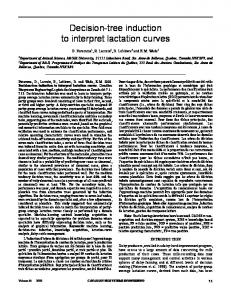
Fig 1.1 Fig1.1. A decision tree for the concept buys computer, indicating whether a customer at All Electronics is likely to purchase a computer. Each internal (nonleaf) node represents a test on an attribute. Each leaf node represents a class (either buys computer = yes or buys computer = no).

(2) if tuples in D are all of the same class, C then

A path is traced from the root to a leaf node, which holds the class prediction for that tuple. Decision trees can easily be converted to classification rules. “Why are decision tree classifiers so popular?” The construction of decision tree classifiers does not require any domain knowledge or parameter setting, and therefore is appropriate for exploratory knowledge discovery.

(6) apply Attribute selection method(D, attribute list) to

3. PROPOSED SYSTEM

(3) return N as a leaf node labeled with the class C; (4) if attribute list is empty then (5) return N as a leaf node labeled with the majority class in D; // majority voting find the “best” splitting criterion; (7) label node N with splitting criterion; (8) if splitting attribute is discrete-valued and multiway splits allowed then // not restricted to binary trees (9) attribute list attribute list _ splitting attribute; // remove splitting attribute

Decision trees can handle high dimensional data. Their representation of acquired knowledge in tree form is intuitive and generally easy to assimilate by humans. The learning and classification steps of decision tree induction are simple and fast. In general, decision tree classifiers have good accuracy. However, successful use may depend on the data at hand. Decision tree induction algorithms have been used for classification in many application areas, such as medicine, manufacturing and production, financial analysis, astronomy, and molecular biology. Decision trees are the basis of several commercial rule induction systems. Algorithm: Generate decision tree. Generate a decision tree from the training tuples of data partition D.

(10) for each outcome j of splitting criterion // partition the tuples and grow subtrees for each partition (11) let Dj be the set of data tuples in D satisfying outcome j; // a partition (12) if Dj is empty then (13) attach a leaf labeled with the majority class in D to node N; (14) else attach the node returned by Generate decision tree(Dj, attribute list) to node N; endfor (15) return N;

Input: Data partition, D, which is a set of training tuples and their associated class labels; attribute list, the set of Most algorithms for decision tree induction also follow such a top-down approach, which starts with a training set of tuples and their associated class labels. The training set is recursively partitioned into smaller subsets as the tree is being built. A basic decision tree algorithm is summarized in Figure 1.1 At first glance, the algorithm may appear long, but fear not! It is quite straightforward.

© 2012, IJARCSSE All Rights Reserved

4. WORKING OF ALGORITHM The strategy is as follows. The algorithm is called with three parameters: D, attribute list, and Attribute selection method. We refer to D as a data partition. Initially, it is the complete set of training tuples and their associated class labels. The parameter attribute list is a list of attributes describing the tuples. Attribute selection method

Page | 428

Volume 2, Issue 4, April 2012 specifies a heuristic procedure for selecting the attribute that ―best‖ discriminates the given tuples according to class. This procedure employs an attribute selection measure, such as information gain or the gini index. Whether the tree is strictly binary is generally driven by the attribute selection measure. Some attribute selection measures, such as the Gini index, enforce the resulting tree to be binary. Others, like information gain, do not, therein allowing multiway splits (i.e., two or more branches to be grown from a node). The tree starts as a single node, N, representing the training tuples in D (step 1).5 If the tuples in D are all of the same class, then node N becomes a leaf and is labeled with that class (steps 2 and 3). Note that steps 4 and 5 are terminating conditions. All of the terminating conditions are explained at the end of the algorithm. Otherwise, the algorithm calls Attribute selection method to determine the splitting Criterion. The splitting criterion tells us which attribute to test at node N by determining the ―best‖ way to separate or partition the tuples in D into individual classes (step 6). The splitting criterion also tells us which branches to grow from node N with respect to the outcomes of the chosen test. More specifically, the splitting criterion indicates the splitting attribute and may also indicate either a split-point or a splitting subset. The splitting criterion is determined so that, ideally, the resulting partitions at each branch are as ―pure‖ as possible. A partition is pure if all of the tuples in it belong to the same class. In other words, if we were to split up the tuples in D according to the mutually exclusive outcomes of the splitting criterion, we hope for the resulting partitions to be as pure as possible. The node N is labeled with the splitting criterion, which serves as a test at the node (step 7). A branch is grown from node N for each of the outcomes of the splitting criterion [7]. The tuples in D are partitioned accordingly (steps 10 to 11). There are three possible scenarios, as illustrated in Figure 1.2 Let A be the splitting attribute. A has v distinct values, f =a1, a2, : : : , avg, based on the training data.1. A is discrete-valued: In this case, the outcomes of the test at node N correspond directly to the known values of A. A branch is created for each known value, aj, of A and labeled with that value (Figure 1.2(a)). Partition Dj is the subset of class-labeled tuples in D having value aj of A. Because all of the tuples in a given partition have the same value for A, then A need not be considered in any future partitioning of the tuples.

© 2012, IJARCSSE All Rights Reserved

www.ijarcsse.com Therefore, it is removed from attribute list (steps 8 to 9). 2. A is continuous-valued: In this case, the test at node N has two possible outcomes, corresponding to the conditions A _ split point and A > split point, respectively, where split point is the split-point returned by Attribute selection method as part of the splitting criterion. Two branches are grown from N and labeled according to the above outcomes (Figure 1.2(b)). The tuples are partitioned such thatD1 holds the subset of class-labeled tuples in D for which A split point, while D2 holds the rest. 3. A is discrete-valued and a binary tree must be produced (as dictated by the attribute selection measure or algorithm being used): The test at node N is of the form ―A 2 SA?‖. SA is the splitting subset for A, returned by Attribute selection method [1] as part of the splitting criterion. It is a subset of the known values of A. If a given tuple has value aj of A and if aj 2 SA, then the test at node N is satisfied. Two branches are grown from N (Figure 1.2(c)). By convention, the left branch out of N is labeled yes so that D1 corresponds to the subset of classlabeled tuples in D that satisfy the test. The right branch out of N is labeled no so that D2 corresponds to the subset of class-labeled tuples [4] from D that do not satisfy the test. The algorithm uses the same process recursively to form a decision tree [2] for the tuple sat each resulting partition, Dj, of D (step 14). The recursive partitioning stops only when any one of the following terminating conditions is true: 1. All of the tuples in partition D (represented at node N) belong to the same class (steps 2 and 3), or 2. There are no remaining attributes on which the tuples may be further partitioned (step 4). In this case, majority voting is employed (step 5). This involves converting node N into a leaf and labeling it with the most common class in D. Alternatively, the class distribution of the node tuples may be stored. 3. There are no tuples for a given branch, that is, a partition Dj is empty (step 12). In this case, a leaf is created with the majority class in D (step 13). The resulting decision tree is returned (step 15).The computational complexity of the algorithm given training set D is O(n_jDj_ log(jDj)), where n is the number of attributes describing the tuples in D and jDj is the number of training tuples in D. This means that the computational cost of growing a tree grows at most n_jDj_log(jDj) with jDj tuples. The proof is left as an exercise for the reader. Incremental versions of decision tree induction have also been proposed. When given new training data, these restructure the decision tree acquired from learning on previous training data, rather than relearning a new tree from scratch.

Page | 429

Volume 2, Issue 4, April 2012

www.ijarcsse.com

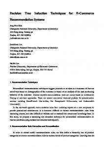
Fig 1.2. Three possibilities for partitioning tuples based on the splitting criterion, shown with examples. Let A be he splitting attribute. (a) If A is discrete-valued, then one branch is grown for each known value of A. (b) If A is continuous-valued, then two branches are grown, corresponding to A _ split point and A > split point. (c) If A is discrete-valued and a binary tree must be produced, then the test is of the form A 2 SA, where SA is the Splitting subset for A. ID3 [10] uses information gain as its attribute selection 4.1 Attribute Selection Measures measure. This measure is based on pioneering work by Claude Shannon on information theory, which studied the An attribute selection measure [3] is a heuristic for value or ―information content‖ of messages. Let node N selecting the splitting criterion that ―best‖ separates a represents or holds the tuples of partition D. The attribute given data partition, D, of class-labeled training tuples [6] with the highest information gain is chosen as the splitting into individual classes. If we were to split D into smaller attribute for node N. This attribute minimizes the partitions according to the outcomes of the splitting information needed to classify the tuples in the resulting criterion, ideally each partition would be pure. The partitions and reflects the least randomness or ―impurity‖ attribute selection measure provides a ranking for each in these partitions. attribute describing the given training tuples. The attribute having the best score for the measure is chosen as the splitting attribute for the given tuples. If the splitting attribute is continuous-valued or if we are restricted to binary trees then, respectively, either a split point or a splitting subset must also be determined as part of the splitting criterion. The tree node created for partition D is labeled with the splitting criterion, branches are grown for each outcome of the criterion, and the tuples are partitioned accordingly. This section describes three popular attribute selection measures—information gain, gain ratio, and gini index. The notation used herein is as follows. Let D, the data partition, be a training set of class-labeled tuples. Suppose the class label attribute has m distinct values defining m distinct classes, Ci (for i = 1, : : : , m). Let Ci,D be the set of tuples of class Ci in D. Let jDj and jCi,Dj denote the number of tuples in D and Ci,D, respectively.

4.1.1 Information gain

© 2012, IJARCSSE All Rights Reserved

Fig 1.3 The attribute age has the highest information gain and therefore becomes the splitting attribute at the root node

Page | 430

Volume 2, Issue 4, April 2012 of the decision tree. Branches are grown for each outcome of age. The tuples are shown partitioned accordingly. Such an approach minimizes the expected number of tests needed to classify a given tuple and guarantees that a simple (but not necessarily the simplest) tree is found. The expected information needed to classify a tuple in D is given by

Where pi is the probability that an arbitrary tuple in D belongs to class Ci and is estimated by jCi, Dj/jDj. A log function to the base 2 is used, because the information is encoded in bits. Info (D) is just the average amount of information needed to identify the class label of a tuple in D. Note that, at this point, the information we have is based solely on the proportions of tuples of each class. Info(D) is also known as the entropy of D.

www.ijarcsse.com having a large number of values. For example, consider an attribute that acts as a unique identifier, such as product ID. A split on product ID would result in a large number of partitions (as many as there are values), each one containing just one tuple. Because each partition is pure, the information required to classify data set D based on this partitioning would be Info product ID(D) = 0. Therefore, the information gained by partitioning on this attribute is maximal. Clearly, such a partitioning is useless for classification. C4.5, a successor of ID3, uses an extension to information gain known as gain ratio, which attempts to overcome this bias. It applies a kind of normalization to information gain using a ―split information‖ value defined analogously with Info(D) as SplitInfoA(D) =

4.1.2 Gain ratio The information gain measure is biased toward tests with many outcomes. That is, it prefers to select attributes This value represents the potential information generated by splitting the training data set, D, into v partitions, corresponding to the v outcomes of a test on attribute A. Note that, for each outcome, it considers the number of tuples having that outcome with respect to the total number of tuples in D.

It differs from information gain, which measures the information with respect to classification that is acquired based on the same partitioning. The gain ratio is defined as above The attribute with the maximum gain ratio is selected as the splitting attribute. Note, however, that as the split information approaches 0, the ratio becomes unstable. A constraint is added to avoid this, whereby the information gain of the test selected must be large—at least as great as the average gain over all tests examined.

4.1.3 Gini index

© 2012, IJARCSSE All Rights Reserved

The Gini index is used in CART [8]. Using the notation described above, the Gini index measures the impurity of D, a data partition or set of training tuples, as

Where pi is the probability that a tuple in D belongs to class Ci and is estimated by jCi, Dj/jDj. The sum is computed over m classes. The Gini index considers a binary split for each attribute. Let’s first consider the case where A is a discrete-valued attribute having v distinct values, fa1, a2, : : : , avg, occurring in D. To determine the best binary split on A, we examine all of the possible subsets that can be formed using known values of A. Each subset, SA, can be considered as a binary test for attribute A of the form ―A 2 SA?‖. Given a tuple, this test is satisfied if the value of A for the tuple is among the values listed in SA. If A has v possible values, then there are 2v possible subsets. For example, if income has three possible values, namely flow, medium, highg, then the possible subsets are flow, medium, high g, flow, medium g, flow, high g, f medium, high g, flow g, f medium g, f high g, and fg. We exclude the power set, flow, medium, high g, and the empty set from consideration since, conceptually, they do not represent a split. Therefore, there are 2v_2 possible ways to form two partitions of the data, D, based on a binary split on A. When considering a binary split, we compute a weighted sum of the impurity of each resulting partition. For

Page | 431

Volume 2, Issue 4, April 2012 example, if a binary split on A partitions D into D1 and D2, the gini index of D given that partitioning is

For each attribute, each of the possible binary splits is considered. For a discrete-valued attribute, the subset that gives the minimum gini index for that attribute is selected as its splitting subset. 4.2 Tree Pruning When a decision tree is built, many of the branches will reflect anomalies in the training data due to noise or

www.ijarcsse.com outliers. Tree pruning methods address this problem of over fitting the data. Such methods typically use statistical measures to remove the least reliable branches. An unpruned tree and a pruned version of it are shown in Figure 1.4. Pruned trees [11] tend to be smaller and less complex and, thus, easier to comprehend. They are usually faster and better at correctly classifying independent test data (i.e., of previously unseen tuples) than unpruned trees. “How does tree pruning work?” There are two common approaches to tree pruning: prepruning and postpruning. In the prepruning approach, a tree is ―pruned‖ by halting its construction early (e.g., by deciding not to further split or partition the subset of training tuples at a given node).

Fig 1.4. An unpruned decision tree and a pruned version of it. 4.3 Scalability and Decision Tree Induction “What if D, the disk-resident training set of class-labeled tuples, does not fit in memory? In other words, how scalable is decision tree induction?” The efficiency of existing decision tree algorithms, such as ID3, C4.5, and CART [3], has been well established for relatively small data sets. Efficiency becomes an issue of concern when these algorithms are applied to the mining of very large real-world databases. The pioneering decision tree algorithms that we have discussed so far have the restriction that the training tuples should reside in memory. In data mining applications, very large training sets of millions of tuples are common. Most often, the training data will not fit in memory!

© 2012, IJARCSSE All Rights Reserved

Page | 432

Volume 2, Issue 4, April 2012

www.ijarcsse.com ―save space‖ included discretizing continuous-valued attributes and sampling data at each node. These techniques, however, still assume that the training set can fit in memory.

Fig1.7

Fig 1.5 An example of sub tree (a) repetition (where an attribute is repeatedly tested along a given branch of the tree, e.g., age) and (b) replication (where duplicate sub trees exist within a tree, such as the sub tree headed by the node ―credit rating?‖).

Fig 1.8 The use of data structures to hold aggregate information regarding the training data are one approach to improving the scalability of decision tree induction.

Fig 1.6 Decision tree construction [1] therefore becomes inefficient due to swapping of the training tuples in and out of main and cache memories. More scalable approaches, capable of handling training data that are too large to fit in memory, are required. Earlier strategies to © 2012, IJARCSSE All Rights Reserved

5. CONCLUSION “What if D, the disk-resident training set of class-labeled tuples, does not fit in memory? In other words, how scalable is decision tree induction?”The pioneering decision tree algorithms that we have discussed so far have the restriction that the training tuples should reside in memory. In data mining applications, very large training sets of millions of tuples

Page | 433

Volume 2, Issue 4, April 2012

www.ijarcsse.com

are common. Most often, the training data will not fit in memory! Decision tree construction therefore becomes inefficient due to swapping of the training tuples in and out of main and cache memories. More scalable approaches, capable of handling training data that are too

large to fit in memory, are required. Earlier strategies to ―save space‖ included discretizing continuous-valued attributes and sampling data at each node. These techniques, however, still assume that the training set can fit in memory.

6. REFERENCES

[11] J. Han, Y. Cai, and N. Cercone. Datadriven discovery of quantitative rules in relational databases. IEEE Trans. Knowledge and Data Engineering, 5:29–40, 1993.

[1] V. K. Vaishnavi, "Multidimensional height-balanced trees," IEEE Trans. Comput., vol. C-33, pp. 334-343, 1984. [2] Tomoki Watanuma, Tomonobu Ozaki, and Takenao Ohkawa. ¯Decision Tree Construction from Multidimensional Structured Data..Sixth IEEE International Conference on Data Mining – Workshop s, 2006.

[12] D. H. Freeman, Jr. Applied Categorical Data Analysis. Marcel Dekker, Inc., New York, NY, 1987.

[3] L. Breiman, J. Friedman, R. Olshen, and C. Stone. Classification of Regression Trees. Wadsworth, 1984. [4] Micheline Kamber, Lara Winstone, Wan Gong, Shang Cheng, Jiawei Han, ¯Generalization and Decision Tree Induction: Efficient Classification in Data Mining., Canada V5A IS6, 1996. [5] J. R. Quinlan. Induction of decision trees. Machine Learning, 1:81–106, 1986. [6] J. R. Quinlan. C4.5: Programs for Machine Learning. Morgan Kaufmann, 1993. [7] L. B. Holder. Intermediate decision trees. In Proc. 14th Intl. Joint Conf. on Artificial Intelligence, pages 1056–1062, Montreal, Canada, Aug 1995. [8] XindongWu · Vipin Kumar · J. Ross Quinlan · Joydeep Ghosh · Qiang Yang · Hiroshi Motoda · Geoffrey J. McLachlan · Angus Ng · Bing Liu · Philip S. Yu · Zhi-Hua Zhou · Michael Steinbach · David J. Hand · Dan Steinberg. A survey paper on ¯Top 10 algorithms in data Mining. 2007. [9] M. Mehta, R. Agrawal, and J. Rissanen. SLIQ: A fast scalable classifier for data mining. In Proc. 1996 Intl. Conf. on Extending Database Technology (EDBT’96), Avignon, France, March 1996. [10] J. Shafer, R. Agrawal, and M. Mehta. SPRINT: A scalable parallel classifier for data mining. In Proc. 22nd Intl. Conf. Very Large Data Bases (VLDB), pages 544– 555, Mumbai (Bombay), India, 1996.

© 2012, IJARCSSE All Rights Reserved

Page | 434