co-simulation of chi and simulink models - CiteSeerX

CO-SIMULATION OF CHI AND SIMULINK MODELS D.A. van Beek1 , A.T. Hofkamp1 , M.A. Reniers2 , J.E. Rooda1 , and R.R.H. Schiffelers1 1

Eindhoven University of Technology, Department of Mechanical Engineering P.O. Box 513 5600 MB Eindhoven, The Netherlands 2 Eindhoven University of Technology, Department of Computer Science P.O. Box 513 5600 MB Eindhoven, The Netherlands [email protected]

(This work has been carried out as part of the Darwin project under the responsibility of the Embedded Systems Institute. This project is partially supported by the Netherlands Ministry of Economic Affairs under the BSIK program, and partially supported by the ITEA project TWINS, number 05004)

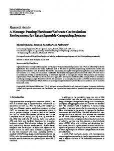
Abstract Using the model-based engineering paradigm for the design of a system, the system is decomposed into several components and models are developed for these components. The models are preferably specified using domain-specific modelling formalisms. By means of co-simulation, the component models can be combined to obtain the overall system behavior. Furthermore, co-simulation enables the reuse and combination of already existing and validated subsystem models without re-entering model data. In this paper, we present a cosimulation framework (see figure at the right) that is based on the S-function interface as present in Matlab Simulink, to simulate models that consist of subsystems modelled using Matlab Simulink and subsystems modelled in the hybrid process algebra Chi (χ ). The principles of the implementation of the framework are described and the framework is illustrated by means of a bottle filling system example.

Simulink Unix process Simulink model a

chi sfunction χ model outputvars = x, y

SimStruct modifications

x y

callback function invocations

callback methods SimStruct modifications

IPC

chi sfunction CMEX

callback function invocations

Python Unix process callback methods TimeStep

chi sfunction Python

Simulate()

χ DE+ simulator TimeStep

GetNextSteps()

DoActionTransition χ model(inputvar a)

Keywords: hybrid systems, model-based engineering, modelling, co-simulation, Chi formalism, Simulink Presenting Author’s Biography Ramon Schiffelers received his Ph.D degree from the Eindhoven University of Technology in February 2006. His thesis was called ’Modelling, Simulation and Verification of Hybrid Systems’. Currently, he is participating in the Darwin project that aims to provide generic methods that will lead to the design of high evolvable systems. He is a member of the (Dutch) Institute for Programming research and Algorithmics (IPA).

1 Introduction In the design cycle of large-scale heterogeneous systems, modelling is a time and labor consuming step. The models generally combine components from many different domains, e.g., hydraulics, thermodynamics, combustion, electronics, supervisory control, scheduling, communication, etc., which have to be described using appropriate formalisms and for which specific software environments exist. Simulation is a popular way of analysing the behavior of the controlled system and it is supported by most of the tools dedicated to hybrid systems. Therefore, in the HYCON NoE [1] as part of work package 3 on tool integration, a study was carried out to provide tool interoperability for simulation purposes. The objective is to increase the modelling efficiency for large-scale heterogeneous systems by enabling • the combination of domain-specific modelling formalisms and component libraries, and • the reuse and combination of already existing and validated subsystem models from different tools without re-entering/re-modelling the model. By means of co-simulation, these objectives can be met. The term co-simulation in this document refers to simulation of a model that consists of different components that may each be simulated by different simulation tools running simultaneously and exchanging information. In literature, the term co-simulation is also used for ‘hardware-software co-simulation’, however such a kind of co-simulation differs from the use in this document. As part of the Darwin project [2], the model-based engineering (MBE) method [3] is used to develop the control system of a patient support system of a MRI scanner. The MBE method is visualized in Figure 1. The system development process is subdivided into multiple (concurrent) component development processes. Subsequently, the resulting components are integrated into the system. Using the MBE approach, the development process of a component C i consists of a requirements definition phase, a design phase, a modelling phase, and a realization phase resulting in the requirements Ri , the design Di , the model Mi , and the realization Z i , respectively. In the development process of a system S that consists of multiple components, e.g. components C1 and C2 , the system requirements R and the system design D precede the development process of the components. The realization of system S is the result of the integration of realizations of Z 1 and Z 2 of the components C1 and C2 by means of infrastructure I12 , denoted by hZ 1 , I12 , Z 2 i. The components might be modelled in several domain-specific modelling formalisms. For example, in case of the patient support system, the physics of the patient support table can be modelled using Simulink [4] (M1 ), and the controller can be modelled using χ [5, 6] (M2 ). By means of co-simulation, the integrated models of the components hM1 , I12 , M2 i can be validated against the system requirements and design.

In this paper, we describe a co-simulation framework based on the S-function interface as available in Matlab Simulink, to simulate models specified in the hybrid process algebra χ. An S-function (system-function) [7] is a computer language description of a MATLAB Simulink block. The form of an S-function is very general and accommodates continuous, discrete, and hybrid systems. The hybrid χ formalism is a hybrid process algebra with a relatively straightforward and elegant syntax and formal semantics that is highly suited to modelling. The intended use of hybrid χ is for modeling, simulation, verification, and real-time control. Its application domain ranges from physical phenomena, such as dry friction, to large and complex manufacturing systems. The semantics of hybrid χ is defined using a structured operational semantics style (SOS) [8]. So far, a χ simulator has been defined and implemented. For this simulator, we derived an implementation from the SOS rules, called the stepper, see [9], and used the symbolic solver from Maple [10]. Based on this same stepper, a χ DE+ (discrete-event-plus) simulator is defined that interacts with Matlab Simulink [4] using an S-function as follows. The DE+ simulator performs (discrete) action transitions until the stepper returns a time step. This time step is returned to Simulink. During the time transition, Simulink solves the equations and monitors the zero-crossings as specified in the time step. At the end of the time transition, the DE+ simulator is called again. This paper is organized as follows. In Section 2, the S-function interface is described. The χ language and the DE+ simulator are described in Section 3. The implementation is described in Section 4, and illustrated by means of an example of a bottle filling system in Section 5. Conclusions are drawn in Section 6.

2

S-function interface

In this section, a brief introduction to S-functions is given, based on [7]. For a comprehensive description of S-functions and their usage with MATLAB Simulink see [7, 4]. An S-function implements a set of methods, called callback methods that together describe the behavior of the (sub) system modelled by means of the S-function. The simulation coordinator, in our case Matlab Simulink, invokes these callback methods during the simulation. 2.1 Specification of an implementation of the Sfunction interface An implementation of the S-function interface must implement the set of callback methods. Some callback methods are optional. The simulation coordinator invokes an optional callback only if the S-function defines the callback. The callback methods perform tasks required at each simulation stage. These tasks performed by the callback methods include: • Initialization. Prior to the first simulation loop, the

Fig. 1 Model-based engineering approach [3]

simulation coordinator initializes the S-function. During this stage: – The SimStruct is initialized. A SimStruct is a simulation structure that contains information about the S-function. – The number and dimensions of input and output ports are set. – The block sample times are set. – The storage areas are allocated. • Calculation of next sample hit. In case a variable sample time block is specified, this stage calculates the time of the next sample hit; that is, it calculates the next step size. • Calculation of outputs in the major time step. After this call is complete, all the output ports of the blocks are valid for the current time step. • Update of discrete states in the major time step. In this call, all blocks should perform once-per-timestep activities such as updating discrete states for next time around the simulation loop. • Integration. This applies to models with continuous states and/or non-sampled zero crossings. If the S-function contains continuous states, the simulation coordinator calls the output and derivative portions of the S-function at minor time steps. In this way, the simulation coordinator can compute the states for the S-function. If the S-function contains non-sampled zero crossings, the simulation coordinator calls the output and zero-crossings portions of the S-function at minor time steps so that the zero crossings can be located. In this paper, we focus on the C implementation of the S-function interface. The main callback functions together with a brief description of their functionality is given in Table 1.

Tab. 1 Functionality of callback methods mdlInitializeSizes Specifies the number of inputs, outputs, states, and parameters and other characteristics of the S-function mdlInitializeSampleTimes Specifies the sample rates mdlInitializeConditions Initializes the state variables mdlOutputs Computes values of the output variables mdlUpdate Updates the state variables mdlDerivatives Computes the derivatives mdlZeroCrossings Updates zero-crossing vector mdlTerminate Performs any actions required at termination of the simulation

S − function, simulation loop S − function, initizalization

Initialization mdlInitializeConditions

mdlInitializeSampleTimes

mdlOutput

To simulation loop

majortimestep

mdlInitializeSizes

mdlUpdate Integration

Fig. 2 Initialization of S-function.

mdlDerivatives

2.2 Interaction of the simulation coordinator with the S-function During simulation, Simulink invokes the predefined set of callback functions of the S-function implementation in order to perform all necessary computations in the right order. Figures 2 and 3 show the order in which the simulation coordinator invokes the callback methods of an S-function, during initialization and simulation respectively. Solid rectangles indicate callbacks that always occur during model initialization and/or at every time step. Dotted rectangles indicate callbacks that may occur during initialization and/or at some or all time steps during the simulation loop.

minortimestep

mdlOutputs

3.1 Syntax A χ model identified by name is of the following form: model name(input i 1 : typei1 , . . . , i k : typeik ) = |[ var s1 : types1 = c1 , . . . , sm : typesm = cm , cont x 1 : typex1 = d1 , . . . , x n : typexn = dn , chan h 1 : typeh 1 , . . . , h q : typeh q , mode X 1 = p1 , . . . , X r = pr :: p ]| Here, typei denotes a type, for instance bool, nat, or real. Notation input i 1 : typei1 , . . . , i k : typeik denotes the declaration of input variables i 1 , . . . , i k . The values of these variables are defined in the environment of the χ model. Notation var s1 : types1 = c1 , . . . , sm : typesm = cm denotes the declaration of discrete variables s1 , . . . , sm with their respective types types1 , . . . , typesm and initial values c1 , . . . , cm . Similarly, notation cont x 1 : typex1 = d1 , . . . , x n : typexn = dn is used to declare continuous variables, and notation chan h 1 : typeh1 , . . . , h q : typehq declares the channels

Zero − crossing detection mdlOutput mdlZeroCrossings mdlTerminate

End Simulation Fig. 3 Simulation stages of S-function.

3 The hybrid χ language and simulator In this section, the syntax and semantics of (a subset of) the hybrid χ language are discussed informally. A more detailed explanation of hybrid χ can be found in [5, 6].

mdlDerivatives

h 1 , . . . , h q . Notation mode X 1 = p1 , . . . , X r = pr declares mode variables X 1 , . . . , X r with their respective statement definitions p1 , . . . , pr . The χ language consists of the following statements p ∈ P:

P

::= | | | | | | | | | | | |

xn := en u delay d X b→P ∗P P; P P8P PkP h ! en h ? xn |[ D :: P ]| lp (en )

(multi-) assignment delay predicate delay statement mode variable guard operator repetition sequential composition alternative composition parallel composition send statement receive statement scope operator process instantiation

Here, xn denotes the (non-dotted) variables x 1 , . . . , x n such that time 6∈ {xn }, en denotes the expressions e1 , . . . , en , u and b are both predicates over variables (including the variable time) and dotted continuous

variables, d denotes a numerical expression, X denotes a mode variable, h denotes a channel, D denotes declarations of local (discrete or continuous) variables, local mode variables, and local channels, and l p denotes a process identifier. The operators are listed in descending order of their binding strength as follows → , ; , {k , 8 }. The operators inside the braces have equal binding strength. For example, x := 1; y := x 8 x := 2; y := 2x means (x := 1; y := x) 8 (x := 2; y := 2x). Parentheses may be used to group statements. To avoid confusion, parenthesis are obligatory when alternative composition and parallel composition are used together. E.g. p 8 q k r is not allowed and should either be written as ( p 8 q) k r , or as p 8 (q k r ). A multi-assignment xn := en denotes the assignment of the values of the expressions en to the variables xn . A delay predicate u, usually in the form of a differential algebraic equation, restricts the allowed behavior of the continuous and algebraic variables in such a way that the value of the predicate remains true over time. A delay statement delay d delays for d time units and then terminates by means of an internal action. Mode variable X denotes a mode variable (identifier) that is defined at the declarations. Among others, it is used to model repetition. Mode variable X can do whatever the statement of its definition can do. The guarded process term b → p can do whatever actions p can do under the condition that the guard b evaluates to true. The guarded process term can delay according to p under the condition that for the intermediate valuations during the delay, the guard b holds. The guarded process term can perform arbitrary delays under the condition that for the intermediate valuations during the delay, possibly excluding the first and last valuation, the guard b does not hold. Repetition ∗ p denotes the infinite repetition of p. Sequential composition operator term p; q behaves as process term p until p terminates, and then continues to behave as process term q. The alternative composition operator term p 8 q models a non-deterministic choice between different actions of a process. With respect to time behavior, the participants in the alternative composition have to synchronize. Parallelism can be specified by means of the parallel composition operator term p k q. Parallel processes interact by means of shared variables or by means of synchronous point-to-point communication/synchronization via a channel. The parallel composition p k q synchronizes the time behavior of p and q, interleaves the action behavior (including the instantaneous changes of variables) of p and q, and synchronizes matching send and receive actions. The synchronization of time behavior means that only the time behaviors that are allowed by both p and q are allowed by their parallel composition.

By means of the send process term h ! en , for n ≥ 1, the values of expressions en (evaluated w.r.t. the extended valuation) are sent via channel h. For n = 0, this reduces to h ! and nothing is sent via the channel. By means of the receive process term h ? xn , for n ≥ 1, values for xn are received from channel h. We assume that all variables in xn are different. For n = 0, this reduces to h ?, and nothing is received via the channel. Communication in χ is the sending of values by one parallel process via a channel to another parallel process, where the received values (if any) are stored in variables. For communication, the acts of sending and receiving (values) have to take place in different parallel processes at the same moment in time. In case no values are sent and received, we refer to synchronization instead of communication. The scope operator |[ D :: P ]| is used to declare a scope consisting of local (discrete or continuous) variables, local mode variables, and local channels. Process instantiation l p (en ) denotes the instantiation of process definition proc l p (fn ) = |[ D :: p ]| that should be defined at the level of the χ model. Here, en and fn denote the actual and formal parameters, respectively. 3.2 Formal semantics The semantics of χ is defined by means of deduction rules in SOS style [8] that associate a hybrid transition system with a χ model as defined in [6]. The hybrid transition system consists of action transitions and time transitions. Action transitions define instantaneous changes, where time does not change, to the values of variables. Time transitions involve the passing of time, where for all variables their trajectory as a function of time is defined. 3.3 Definition of the stepper The stepper computes the set of possible transitions given a χ process. The stepper consists of three main functions: function Sa which returns the set of action steps given a χ process, function Sd which returns the set of time steps given a χ process, and function Tr which returns the set of transitions given a step. Action steps and time steps can be seen as symbolic transitions. They consist of all information needed to determine the transitions that the process from which they are derived can perform. An action step represents zero or more action transitions and a time step represents zero or more time transitions. An action step (c, W, r, l a , p0 ) consists of the condition (guards) c that should hold, the set of variables W that may change, the predicate r describing (restricting) the discrete updates, the performed action label l a , and the resulting process term p0 . A time step (c [0] , c(0,t), c[t] , c[0,t], c, p0 ) consists of the predicate c [0] that should hold at the start point of the time transitions, the predicate c (0,t) that should hold at all time points between the start- and endpoint of the time transitions, the predicate c [t] that should hold at the endpoint of the time transitions, the predicate c [0,t] that should hold at all time points (including the startand endpoint) of the time transitions, the predicate c

that should hold at least at one time point of the time transition, and the resulting process term p 0 . 3.4 DE+ simulator The stepper functions are defined in such a way that it is easy to define the DE+ (discrete-event-plus) simulator. This simulator interacts with Matlab Simulink using an S-function as follows. The DE+ simulator performs action transitions until the stepper returns a time step. This time step is returned to Simulink. During the time transition, Simulink solves the delay predicates as specified in the time step. At the end of the time transition, the DE+ simulator is called again. The DE simulator consists of a function Simulate, which is defined as follows: Simulate(M) = while M 6= X Sdo atrans := astep∈Sa (M) Tr (astep) if atrans 6= ∅ then M := DoActionTrans(pick(atrans)) else dsteps := Sd (M) if dsteps 6= ∅ then return pick(dsteps) else return deadlock endif endif endwhile return stop simulation +

as a generic piece of software, independent of a specific χ model. Also, a tool set exists that translates a χ model to a form usable for the stepper. The generic stepper software together with the translated χ model provides action transitions, termination transitions, and time transitions specific for the χ model. The C programming language [12] was used for connecting to the callback methods in the Simulink program. The following questions thus needed to be answered. • In which language to write the DE+ simulator and the χ S-function callback methods? • How/where to run the Python interpreter?

If the set of action transitions is empty, the possible delay steps (dsteps) that the process can perform are calculated. If the set of delay steps is empty, the process is deadlocked. If the set of delay steps is not empty, a delay step is selected and returned. If the model is terminated (M = X), a request is sent to the simulation coordinator to stop the simulation (stop simulation).

Both the DE+ simulator and the χ S-function callback methods deal with equations and values of variables. They must evaluate expressions in order to decide what reply to give to each callback method. Coding these in C implies that expressions need to be transfered between Python and C. Also, an expression evaluator would need to be implemented in C, functionality already present in the simulator. (Note that like the stepper software, the coupling with the χ S-function methods is generic software, that is, without knowledge about which χ model will be used. Techniques such as compiling expressions to C into the S-function block can therefore not be employed.) Coding the DE+ simulator and the χ S-function callback methods in Python implies that vectors/arrays of reals or integers need to be transfered between Python and C, a problem much more manageable than handling expressions and evaluating them, in C. The decision was thus made to implement both the DE+ simulator and the χ S-function callback methods in Python. In other words, calls received from the S-function methods in C are first forwarded to Python, the Python implementation of the S-function methods computes the answer using the DE+ simulator, and finally, the result is transfered back to C and delivered to Simulink. This solution results in a framework of interfacing to S-function methods in Python which is independent of its application (such as connecting to the DE+ simulator). We may find other uses for this framework in the future.

4 Implementation

The question of how/where to run the Python interpreter boils down to two options.

Given a χ model M, all possible action transitions are calculated and stored in variable atrans. If the set of action transitions is not empty, an action transition is selected (non-deterministically) and performed resulting in the new state M (M := DoActionTrans(pick(atrans))). Then, the simulate function is applied on the new state M.

Realization of the co-simulation means that the stepper for χ models has to be implemented. On top of the stepper functions the DE+ simulator has to be built, and finally callback functions from the S-function interface are implemented using the Simulate() function. The design considerations of the framework are discussed in Section 4.1. In Section 4.2, the implementation of the callback methods of the chi sfunction block is described. 4.1 Design considerations In our case, a simulator using the stepper was already implemented in the programming language Python [11]

• Embed the interpreter in the Simulink program. • Run the interpreter as a separate Unix process. Python is designed to act as glue between other software, so embedding it in other software is in itself no problem. However, you can have only one Python interpreter in a single operating system process. Use of multiple χ S-function blocks (each with its own χ model) in the same simulation can only be supported by running multiple Python threads (inside the interpreter). Such thread information would typically be stored as

part of the Simstruct data, and would need to travel over the C/Python connection, making the generic call forwarding framework more complex. Also, in an earlier experiment, we experienced clashes between the dynamic module loading mechanism of Matlab/Simulink and Python of which we are unsure how to deal with, but we consider this to be a non-critical issue for now. The other alternative, running a Python interpreter as separate Unix process for each S-function block, and connect them to the S-function interface using Inter Process Communication (IPC) is a proven technology explained in many books (for example [13]) that allows as many concurrent χ S-function blocks as the machine allows new processes without any of the threading and/or dynamic loading troubles. In addition, the Python side of the call forwarding framework becomes a normal Python extension, which makes it easier to use and support. The decision was made to have one Python Unix process running the stepper and the DE+ simulator for each χ S-function block. The IPC mechanisms that are potentially useful are • Sockets: Network-enabled, more complex to setup connection, sockets are managed by the operating system. • (Named) pipes: Fast, not over the network, pipes are managed by the operating system. • Shared memory: Very fast, not over the network, needs additional read/write access control, memory blocks need separate management. We selected (named) pipes as IPC mechanism for their simplicity. The additional complexity of sockets gives no additional advantages. If we encounter performance problems due to IPC, we can always switch to shared memory. The result of these decisions together is visualized in Figure 4. Inside the Simulink model, many blocks can be used to model a system, including one or more χ S-function blocks. For each χ S-function block, the call forwarding framework is instantiated. A Python interpreter is started as a separate Unix process, and two pipes are created between them (one for forwarding Sfunction method parameters to the Python interpreter, and one for sending results back). At the Python side, the S-function methods are implemented by using the DE+ simulator, the stepper, and the compiled χ model. 4.2 Implementation of the chi sfunction callback methods The implementation of the callback methods of the chi sfunction block are defined as follows. mdlInitializeSizes The pipes are created, the Python interpreter is initialized (forked) and the χ model is instantiated. The discrete variables of the χ process are mapped to the discrete state variables of the S-function block. The continuous variables and the variable time of the χ process are mapped to the continuous state variables of

Simulink Unix process Simulink model

a

chi sfunction χ model outputvars = x, y

SimStruct modifications

x y

callback function invocations

callback methods SimStruct modifications

IPC

chi sfunction CMEX

callback function invocations

Python Unix process callback methods TimeStep

chi sfunction Python

Simulate()

χDE+ simulator TimeStep

GetNextSteps()

DoActionTransition χ model(inputvar a) Fig. 4 Process model of the framework.

the S-function block. The number of input ports is set to the number of input variables that are specified in the formal parameter list of the χ model. The number of output ports is set to the number of output variables as specified in the parameters of the chi sfunction block. The number of Sample Times is set to 1. The number of zero crossings is set to the number of occurrences of guard operators plus the number of occurrences of inequality delay predicates plus 1 for the time events. Using pseudo code, the implementation of function mdlInitializeSizes is as follows: global TimeStep chimodel = GetChiModel() mapVariables() mdlInitializeSampleTimes The sample time of the S-function is set to a continuous sample time with offset 0. mdlInitializeConditions The initial values for the state variables from the Sfunction are obtained from the valuation from the χ process, using the variable mapping as defined in function mdlInitializeSizes.

where function GetEquations projects the equalities from a time step. mdlZeroCrossings The inequality conditions (zero-crossing conditions) are obtained from the time step. Using pseudo code, the implementation of function mdlZeroCrossings is as follows: ZeroCrossings := GetZeroCrossings(TimeStep), where function GetZeroCrossings projects the inequalities from a time step. mdlTerminate Using this function stops the Python interpreter and closes the pipes.

5

Example

The bottle filling system as shown in Figure 5 consists of a liquid storage tank, two identical bottle filling lines, and a bottle supply (see [6]).

mdlOutputs The values of the discrete and continuous variables and the variable time are copied to the corresponding output variables. If the simulation step is a major time-step, it is determined whether a time event occurred.

Qa

Qu V Q Fl

Q Fr

mdlUpdate If the mdlUpdate function is called for the first time (ssIsFirstInitCond(S) holds, where S denotes the SimStruct), the χ process is simulated using the DE+ simulator. If a time event occurred (IsTimeEvent holds), which is determined in function mdlOutputs, the resulting process is obtained using the end-valuation of the time transition (EndState(TimeStep)). After that, this process is simulated using the DE+ simulator. Using pseudo code, the implementation of function mdlUpdate is as follows: if ssIsFirstInitCond(S) then TimeStep := Simulate(M) else if IsTimeEvent then TimeStep := Simulate(EndState(TimeStep)) endif endif mdlDerivatives The equality conditions from the time step are used to obtain the values for the derivatives of the continuous state variables of the S-function. The χ model is restricted in such way that these equality equations together form an ODE. Using pseudo code, the implementation of function mdlDerivatives is as follows: Equations := GetEquations(TimeStep),

Fig. 5 The bottle filling system.

The bottles are filled with liquid from the storage tank. A control system keeps the volume V in the storage tank between 2 and 10. The liquid supply processes is not modeled, since we consider the liquid always to be available, and we are not interested in the amount of liquid that is used. The Simulink model of the bottle filling system is shown in Figure 6. The dynamics of the liquid storage tank are modelled in Simulink. The volume controller is modelled in χ, see below: model VC(input V : real)= |[ var beta : nat = 0 :: *( V beta := 1 ; V >= 10.0 -> beta := 0 ) ]|

The behavior of the volume controller VC is explained as follows. Initially, the volume V in the storage tank equals 10. If the volume drops below the minimum

, filling

beta

1.5 Qsetu

Qu chi_sfunction Volume controller Chi

Vdot

Subtract

, finished

1 s Integrator

V

, stopped :: get_crate ]|

= QF:=1.0 ; ( V QF := 0.0 ; stopped | Vb >= 1.0 -> QF := 0.0 ; finished ) = n := n - 1 ; ( n = 0 -> get_crate | n >= 1 -> Vb := 0.0 ; filling ) = V >= 0.7 -> filling

]| proc Bottle_Supply(chan bottles! : nat) = |[ *( bottles!6; delay 5.0 ) ]|

QF_l QF_r Vb_l

Vb_l

Vb_r

chi_sfunction Filling Lines Chi

Vb_r

Fig. 6 Simulink model of the bottle filling system.

value 2 (V= Vset -> bottles?n ; Vb := 0.0 ; filling

Model FillingLines consists of two controlled filling lines CLine(Vb l, QF l, bottles, 0.0), CLine(Vb r, QF r, bottles, 5.0) and a bottle supply process Bottle Supply(bottles). Repeatedly the bottle supply process sends 6 bottles via channel bottles (bottles!6), and 5 time units later (delay 5.0), it tries to send 6 bottles again. The behavior of a controlled filling line CLine is explained as follows. In mode get crate, the process waits until the volume in the storage tanks exceeds Vset, and a new crate of bottles arrives, (bottles?n, where n denotes the number of bottles in a crate). Then, the bottle volume is reset to 0 resulting in mode filling. In mode filling, the valve is opened (QF:=1.0) starting the filling process. Filling stops when the volume in the storage tank drops below 0.5 (V QF := 0.0; stopped). In mode stopped, filling resumes when the volume in the storage tank is at least 0.7 (V >= 0.7 -> filling). Filling also stops when the bottle is full (Vb >= 1.0 -> QF := 0.0; finished). In mode finished, the number of bottles to be filled (modelled by variable n) is decreased by 1. If the number of bottles equals 0, a new crate is requested, otherwise the bottle volume is reset, and filling of the new bottle is started. Figures 7 and 8 show the simulation results for the volume V in the liquid storage tank and the incoming flow Q u , respectively.

6

Conclusions

In this paper, we presented a framework to simulate models that consist of subsystems modelled using Matlab Simulink and subsystems modelled in the hybrid process algebra Chi (χ). Its implementation and its use is illustrated by means of a bottle filling system example. Future work entails, amongst others, to explore the possibilities of using this approach in a real-time setting using Matlab Simulinks Real-Time-Workshop. The Sfunction approach, as described in this paper, also enables co-simulation with other simulators that can interface with S-functions. For instance, in the HYCON

NoE, the Modelica language [14, 15] will be extended with an interface to simulate S-functions. In the Darwin project, by means of co-simulation, the integrated models of the components of the patient support table can be validated against the system requirements and design.

7

10 9 8

V

7 6 5 4 3 2 1 0

20

40

60

80

100

time

Fig. 7 Volume V in the liquid storage tank.

1.6 1.4 1.2 Qu

1 0.8 0.6 0.4 0.2 0 0

20

40

60 time

Fig. 8 Incoming flow Q u .

80

100

References

[1] HYCON Network of Excellence. http://www.isthycon.org/, 2005. [2] Darwin project. http://www.esi.nl/site/projects/darwin.html, 2006. [3] N. C. W. M. Braspenning, J. M. van de MortelFronczak, and J. E. Rooda. A model-based integration and testing method to reduce system development effort. Electronic Notes in Theoretical Computer Science, 164:13–28, 2006. [4] The MathWorks, Inc. Using Simulink, version 6. http://www.mathworks.com, 2005. [5] D. A. van Beek, K. L. Man, M. A. Reniers, J. E. Rooda, and R. R. H. Schiffelers. Syntax and consistent equation semantics of hybrid Chi. Journal of Logic and Algebraic Programming, 68(12):129–210, 2006. [6] K. L. Man and R. R. H. Schiffelers. Formal Specification and Analysis of Hybrid Systems. PhD thesis, Eindhoven University of Technology, 2006. [7] The MathWorks, Inc. Writing S-functions, version 6. http://www.mathworks.com, 2005. [8] Gordon D. Plotkin. A structural approach to operational semantics. Journal of Logic and Algebraic Programming, 60-61:17–139, 2004. [9] D. A. van Beek, K.L. Man, M. A. Reniers, J. E. Rooda, and R. R. H. Schiffelers. Deriving simulators for hybrid Chi models. In IEEE International Symposium on Computer-Aided Control Systems Design, pages 42–49, Munich, Germany, 2006. IEEE. [10] MapleSoft. http://www.maplesoft.com, 2005. [11] Python. http://www.python.org, 2005. [12] Brian W. Kernighan and Dennis M. Ritchie. The C programming language. Prentice Hall, second edition, 1988. [13] W. Richard Stevens. Advanced programming in the unix environment. Addison Wesley, 1993. [14] Sven Erik Mattsson, Martin Otter, and Hilding Elmqvist. Modelica hybrid modeling and efficient simulation. In 38th IEEE Conference on Decision and Control, pages 3502–3507, 1999. [15] Modelica Association. Modelica - A Unified Object-Oriented Language for Physical Systems Modeling. http://www.modelica.org, 2002.