Mecánica Computacional Vol XXXIII, págs. 3003-3015 (artículo completo) Graciela Bertolino, Mariano Cantero, Mario Storti y Federico Teruel (Eds.) San Carlos de Bariloche, 23-26 Setiembre 2014
COLLISION PROBABILITIES METHOD EXTENTION FOR SIMPLIFIED 3-D GEOMETRIES Diego Ferraroa and Eduardo Villarinob a
Nuclear Engineering Department, INVAP S.E, Esmeralda 356, Buenos Aires, Argentina,
[email protected]
b
Nuclear Engineering Department, INVAP S.E, Av. Comandante Luis Piedrabuena 4950, Bariloche, Río Negro, Argentina,
[email protected]
Keywords: CONDOR neutronic calculation code, HRM method, Collision Probabilities Abstract. To solve the neutron transport equation at general 2-D geometries the cell-level code CONDOR v. 2.7.01 (E.A. Villarino 2002) uses a method which couples spatial elements using neutron currents, which had been previously calculated by the Collision Probabilities method. Such methodology, usually known as Heterogeneous Response Method (HRM) has been shown as a powerful method to solve complex geometries with high reduction of the computational resources, where the most relevant effort was carried out in past decades to obtain a well-optimized and stable ray-tracing method to perform the CP calculations on each spatial element (E. A. Villarino, R. Stamm´ler, A. Ferri & J. Casal 1992). Nevertheless, the current development of Fuel Assemblies, in-core and ex-core devices (mainly for Research Reactors) with high axial heterogeneity is demanding a 3-D extension of current methods available. Unfortunately, develop a general 3-D HRM method, leads to the development of a complete new ray-tracing scheme and implies a big implementation and validation effort. Furthermore, most calculations at cell level do not need high complex 3-D geometries. The present work, developed in the framework of the Upgrade of INVAP´s proprietary calculation line developed with the contribution of the Argentine National Agency of Technological and Scientific Promotion (Agencia Nacional de Promoción Científica y Tecnológica -ANPCyT), through the funds of the Argentine Technological Funds (Fondo Tecnológico Argentino, FONTAR), presents the basics of an alternative solution for the 3-D problem extension, that considers only an axial extension of the HRM method, in order to be included in CONDOR code in the near future. Furthermore, this method is intended to allow the modeling of most of cases of interest at cell-level Accordingly, the theoretical basis for the HRM extension to simplified 3-D geometries is presented, where the coupling with already optimized 2-D ray-tracing is presented and several proposals for implementation are presented.
Copyright © 2014 Asociación Argentina de Mecánica Computacional http://www.amcaonline.org.ar
3004
1
D. FERRARO, E. VILLARINO
INTRODUCTION
To model, design and optimize complex nuclear core reactors, INVAP uses its ownproprietary developed CONDOR v. 2.7.01 cell-level code (E. Villarino 2002), included into the INVAP reactor calculation package (I. Mochi 2010). This cell code is used to perform neutronic calculations at cell level for fuel assemblies and devices included in the core of a nuclear reactor, in order to produce the required data (such as homogenized and condensed cross-sections) to be used in a reactor core-level code. To solve the neutron transport equation at cell level, CONDOR v. 2.7.01 includes several alternatives based in the Collision Probabilities Method (R. J. J. Stamm’ler and M. J Abbate, 1983). Thus CONDOR v. 2.7.01 includes slab and cylindrical 1-D solver, a cylindrical 2-D solver and a general 2-D geometry solver. The last one, usually named as Heterogeneous Response Method (HRM) is based in the coupling via neutron currents of previously calculated spatial elements calculated by a traditional CP method. This method was firstly introduced in the Helios code (E. A. Villarino, Rudi J. J. Stamm’ler and Aldo A. Ferri 1992) and nowadays is used in several Collision Probabilities cell codes around the world. The HRM methodology has been shown as a powerful method to solve complex geometries with high reduction of the computational resources, where the most relevant effort was carried out in past decades to obtain a well-optimized and stable ray-tracing method to perform the CP calculations on each spatial element. Unfortunately, the current development of Fuel Assemblies, in-core and ex-core devices (mainly for Research Reactors) with high axial heterogeneity is demanding a 3-D extension of the methods available. When this problem is presented, several alternatives can be conceptually analyzed: a) Develop a general 3-D HRM method, where a general 3-D geometry is proposed for each spatial element and then a general coupling is performed. This option leads to a complete new ray-tracing development and a high increase of computational effort. Furthermore, most calculations at cell level do not need highly complex 3-D modeling geometries. b) Develop an axial extension of the well developed HRM 2-D method, where the already optimized 2-D ray tracing is extended to be used in extruded geometries and changes in axial compositions are allowed. Furthermore, this axial heterogeneity allows the modeling of most of cases of interest at cell-level. In the present work, the second option was chosen to be developed, looking for a nearfuture implementation in CONDOR cell code. It should be noted that second option allows an easy adaptation to the actual CONDOR code (I.Mochi 2010) preserving its main capabilities such as Sub-Group Resonant Treatment, Burnup calculations, user-oriented free format input, variational methods, etc. Reader should notice in this point that an axial macroband integration must be considered for this extension, together with an integration scheme to consider the polar angle numerical integration (not performed in 2-D cases). Accordingly, in this work, the main theoretical basis is presented, together with some implementation aspects. 2
AXIAL EXTENSION OF HRM METHOD
2.1 HRM method basics: The local and global problem The Heterogeneous Response Method was developed to solve complex geometry problems in 2-D reducing the computational effort. The approach proposed in the HRM
Copyright © 2014 Asociación Argentina de Mecánica Computacional http://www.amcaonline.org.ar
Mecánica Computacional Vol XXXIII, págs. 3003-3015 (2014)
3005
consists of a first step where the whole geometry is divided in several simple elements to couple them in a second step using the neutron currents. Accordingly, in HRM the whole system is divided into heterogeneous space elements and each heterogeneous element is partitioned in homogeneous regions (namely regions indexed as i,j) where the flat flux approximation is applied (R. J. J. Stamm’ler and M. J Abbate, 1983). In addition, the external surface is also partitioned in segments (indexed with s or t), on which flat coupling currents are calculated, where each segment can be partitioned in azimuthal sectors. Finally, the neutron flux calculation of the system is performed coupling the response fluxes of each element, using the relation presented in matricial notation in Equation 1 (E.A.Villarino, 2002). 𝜙 = 𝑋𝑄 + 𝑌𝑗 (1) Where: : is the volume integrated flux array, where each position i is the integrated flux in region i (for a given Energy group). X: is the matrix of source response fluxes, where the element Xij is the volume integrated flux in region i due to a unit uniform and isotropic source in region j. Q: is the volume integrated source array, where the element Qj is the source in region j. Y: is the matrix of in-current response fluxes, where the element Yis is the volume integrated flux in region i due to a unit in-current through sector s. 𝑗: is the in-current array, where the element 𝑗s is the in-current through sector s. It should be noted here that X and Y are diagonal block matrices, where each block is the local matrix of a previously defined space element. In order to obtain the fluxes by group on each region defined for each element, the Equation 1 is to be solved and two levels of the whole problem emerge: a) Global problem: That consists of coupling the elements, i.e. to calculate the coupling or interfaces currents between previously defined space elements 𝑗. b) Local problem: That consists of solve each element, i.e. to calculate the response fluxes X and Y and multiple collision probabilities of the all space elements. It can be seen here that the extension to a 3-D geometry only implies an effort in the redefinition of the local problem. Afterwards the solution of the global problem should be quite straight forward, where the only apparent implication would be the increase in the computational effort. 2.2 Theoretical Basis for the HRM 2-D case To obtain the collision probabilities for a 2-D element in CONDOR, a 2-D ray tracing is used (E. A. Villarino, Rudi J. J. Stamm’ler and Aldo A. Ferri 1992), which is based in the well known Carlvik method (Carlvik 1965), where a macroband algorithm is applied and a double numerical integration is performed. Afterwards, the program applies normalization schemes on integration chords in order to preserve region volumes and surfaces. This ray-tracing is performed for a given element, where translation and rotations are performed to obtain the optical thicknesses necessary to calculate the surface to region, region to region and surface to surface probabilities. An example is shown in Figure 1, where the nomenclature identifies i and j as regions, k and s as surfaces and i and yi as integration parameters to be used in the double numerical integration.
Copyright © 2014 Asociación Argentina de Mecánica Computacional http://www.amcaonline.org.ar
3006
D. FERRARO, E. VILLARINO
i
ij
j
i
is
s
y
i
j
j
yi i
j
s k
i
s
i
Figure 1 Example of a chord for an integration angle i and position yi
Afterwards, using the thicknesses for each angle and position, the final collision probabilities are obtained just using a weight scheme. For example, to calculate the region to region collision probability, the thicknesses from the left scheme in Figure 1 is used, as it is presented in Equation 2. 𝑝𝑖𝑗 = 𝛼 𝑖 𝑡𝑖 𝑤𝛼 𝑖 𝑤𝑦 𝑖 𝑝𝑖𝑗 (𝛼𝑖 , 𝑦𝑖 ) (2) Here, pij is the probability for a neutron born uniformly and isotropic in region i to suffer its first collision in region j, and wi and wyi represent the weight values for a given angular and position respectively. It should be noted that the same scheme is used to calculate the surface to region probability (middle scheme in Figure 1) and surface to surface probability (right scheme in Figure 1), where instead of pij(i,ti), the pis(i,ti) or pks(i,ti) are calculated. Finally, to calculate pij(i,ti), pis(i,ti) or pks(i,ti), the Equation 3 (R. J. J. Stamm’ler and M. J Abbate, 1983) which represents the probability density function of a neutron emitted in a isotropic line source that travels mean free paths (mfp) without collision, should be integrated using the thicknesses from Figure 1. 𝑝 𝜏, 𝜑, 𝜃 =
cos 𝜃 𝑑𝜃 𝑑𝜑 4𝜋
𝜏
𝑒 (− 𝑐𝑜𝑠𝜃 )
(3)
Here is the polar angle of the chord with the 2-D plane in Figure 1, and it respective azimuthal angle. It should be noted that for a 2-D case, the integration in the angle leads to the well known Bickey order 3 functions. Reader should notice in this point that the region to region collision probabilities will have to be integrated considering chords that sample correctly the volumes of the regions, while the surface to region and surface to surface collision probabilities will need chords that sample the element surfaces. Accordingly, the ray-tracing included in CONDOR v. 2.7.01 consist of two sets of chords constructed for several (i,yi), namely: a) Volume chords: These chords sample preferably the volumes of the regions for the element where the collision probabilities are to be defined (i.e. surfaces for a 2-D case). Additionally, the normalization is chosen as in equation 4. j Voli = j Wj (αi , yi ) thi (4) Copyright © 2014 Asociación Argentina de Mecánica Computacional http://www.amcaonline.org.ar
Mecánica Computacional Vol XXXIII, págs. 3003-3015 (2014)
3007
Here, Voli is the volume of region i, j the total chord number, Wj the weight of each chord (combining i and yi) and thij the sampled thickness of region i in chord j. b) Surface chords: These chords sample preferably the external surface of the element where the collision probabilities are to be obtained (i.e. the perimeter for a 2-D case) Additionally, the normalization is chosen as in equation 5. π Ak = 2 j Wj (αi , yi ) δ(sectorj − sectork ) (5) Here, Ak is the area of sector k (perimeter for a 2-D case), j the total number of chords, and Wj the weight of each chord (combining i and yi), where the sum is over the chords with k as incoming surface (represented as a Kroneker ). Finally, CONDOR uses the volume chords to calculate the region to region collision probabilities through a specific FORTRAN routine (called FREPIJ) and the surface chords to calculate the surface to region and surface to surface probabilities using another one (called TH1GAM). Afterwards the obtained results are normalized in order to satisfy the balances (E. A. Villarino, Rudi J. J. Stamm’ler and Aldo A. Ferri 1992). 2.3 Theoretical Basis for axial extension of the 2-D case In order to extend the method discussed in Sections 2.1 and 2.2 to a 3-D case an axial expansion is proposed. Thus, the original 2-D scheme is extruded in the axial dimension, where only changes in axial composition are allowed, as it is shown in Figure 2. Axial extended 2-D Case
z 2-D Case
Figure 2 Example of an axial extension for a given geometry
As it has been discussed in Section 2.1, the local problem has to be re-defined. To obtain the Collision Probabilities for each axial-extended element, the proposed methodology is to extend the original 2-D chords considering several axial positions and polar angles, as it is shown in Figure 3, where an axial expansion for a given 2-D chord is presented. It can be seen that a new set of regions and surfaces appear when this extension is proposed, where top and bottom surfaces are now considered. Additionally, the integration over the polar angle is not implicit (i.e. Bickley functions are not obtained), thus for each chord, the polar variable must be considered.
Copyright © 2014 Asociación Argentina de Mecánica Computacional http://www.amcaonline.org.ar
3008
D. FERRARO, E. VILLARINO
y
z
k
yi
j
Top surfaces of extension
s
i
i
k
i
s j
Axial expansion for 2-D chord
Bottom surfaces of extension
Figure 3 Example of a chord for an integration angle i and yi extended in axial dimension
2.3.1 Region to Region Collision probabilities for axial extended chords Using the axial extended 2-D chord, the region to region collision probabilities can be obtained from the integration of Equation 6 (E. A. Villarino, Rudi J. J. Stamm’ler and Aldo A. Ferri 1992). 𝑝𝑖𝑗 =
2𝜋 𝑦𝑚𝑎𝑥 𝑦 𝑚𝑖𝑛 2𝜋V i Σ 𝑖 0 1
𝑧 𝑚𝑎𝑥 𝑧 𝑚𝑖𝑛
𝜋/2 𝑡𝑖 −𝜋/2 0
𝑒
−
Σ 𝑖 𝑡 𝑖 −𝑡 +𝜏 𝑖𝑗 cos 𝜃
−𝑒
−
Σ 𝑖 𝑡 𝑖 −𝑡 +𝜏 𝑖𝑗 +𝜏 𝑗 cos 𝜃
cos 𝜃 𝑑𝜃𝑑𝑡𝑑𝑧𝑑𝑦𝑑𝛼
(6)
When the integration over the chord thickness is performed, we obtain the expression we are looking for, presented in Equation 7. 𝑝𝑗𝑖 =
2𝜋 𝑦𝑚𝑎 𝑥 𝑧 𝑚𝑎𝑥 𝑦 𝑚𝑖𝑛 𝑧 𝑚𝑖𝑛 2𝜋V i Σ 𝑖 0 1
𝜋/2 −𝜋/2
𝑒−
𝜏 𝑖𝑗 cos 𝜃
−𝑒
−
𝜏 𝑖𝑗 +𝜏 𝑗 cos 𝜃
+𝑒
−
𝜏 𝑖 +𝜏 𝑖𝑗 +𝜏 𝑗 cos 𝜃
−𝑒
−
𝜏 𝑖𝑗 +𝜏 𝑗 cos 𝜃
cos 2 θ𝑑𝜃𝑑𝑧𝑑𝑦𝑑𝛼
(7)
Besides, to obtain the self-collision probability (i.e. from region i to region i), we can perform the simplification over Equation 6 to obtain Equation 8. 𝑝𝑖𝑖 = 1 −
2𝜋 𝑦𝑚𝑎𝑥 𝑦 𝑚𝑖𝑛 2𝜋V i Σ 𝑖 0 1
𝑧 𝑚𝑎𝑥 𝑧 𝑚𝑖𝑛
𝜋/2 −𝜋/2
1 − 𝑒−
𝜏𝑖 cos 𝜃
cos 2 θ𝑑𝜃𝑑𝑧𝑑𝑦𝑑𝛼
(8)
2.3.2 Surface to Region Collision probabilities for axial extended chords Using the axial extended 2-D chord, the surface to region collision probabilities can be obtained from an integration similar to Equation 6 (E. A. Villarino, Rudi J. J. Stamm’ler and Aldo A. Ferri 1992). Now the incoming surfaces segments (named as sk) are considered. The obtained result is presented in Equation 9, where reader should note that only one azimuthal angle is considered (i.e. no dependence in ), which will lead to couple segments with the white current approximation. 𝜋 𝐴 𝑠 ±𝜋 0 0 0
𝑝𝑠𝑘,𝑖 =
𝜏 𝑖𝑠
𝜏 𝑖𝑠 +𝜏 𝑖
− − cos 𝜃 2 𝑒 cos 𝜃 −𝑒 cos 𝜃
𝑑𝜃 𝑑𝑦𝑑𝜑
𝜋𝐴𝑠 2
(9)
2.3.3 Surface to Surface Collision probabilities for axial extended chords Analogous to Section 2.3.2, using the axial extended 2-D chord, the surface to surface collision probabilities can be obtained from an integration similar to Equation 6 (E. A. Villarino, Rudi J. J. Stamm’ler and Aldo A. Ferri 1992). For this case the incoming and out coming surfaces segments (named as sk and tl respectively) are considered. The obtained result is presented in Equation 10, where reader should note that only one azimuthal angle is considered (i.e. no dependence in ), which will lead to couple segments with the white current approximation.
Copyright © 2014 Asociación Argentina de Mecánica Computacional http://www.amcaonline.org.ar
Mecánica Computacional Vol XXXIII, págs. 3003-3015 (2014)
𝑝𝑠𝑘,𝑡𝑙 = 3
𝜋 𝐴 𝑠 ±𝜋 0 0 0
3009
𝜏𝑠
− cos 𝜃 2 𝑒 cos 𝜃
𝑑𝜃 𝑑𝑦𝑑𝜑
𝜋𝐴𝑠 2
(10)
IMPLEMENTATION
3.1 Main Implementation Equations 7, 8, 9 and 10 are intended to be solved with the available data in CONDOR, without extensive modifications to the main code. Thus, the following scheme was proposed: a) To calculate the region to region probabilities, the original optimized FORTRAN routine FREPIJ (that uses the Bickey functions) was extended to the FREPIJ_3D routine, which includes the extension of the set of 2-D volume chords. b) To calculate the surface to region and surface to surface probabilities for neutrons from the lateral surfaces, the original optimized routine TH1GAM (that uses the Bickey functions) was extended to the TH1GAM_3D routine, which includes the extension of the set of 2-D surface chords. c) To calculate the surface to region and surface to surface probabilities for neutrons from the top and bottom surfaces, the same extended TH1GAM_3D routine was used, but special extended chords were considered, where the original 2-D volume chords where used. τ
For these three cases, the original Bickey functions are replaced by the cos2 𝜃𝑒 − cos 𝜃 term in equations 7, 8, 9 and 10. Besides a numerical integration over the polar angle and axial position appears, thus the scheme presented in Equation 2 has to be extended to Equation 11. 𝑝𝑖𝑗 = 𝜃 𝑖 𝑧 𝑖 𝛼 𝑖 𝑡𝑖 𝑤𝜃 𝑖 𝑤𝑧𝑖 𝑤𝛼 𝑖 𝑤𝑡𝑖 𝑝𝑖𝑗 (𝛼𝑖 , 𝑦𝑖 , 𝜃𝑖, 𝑧𝑖 ) (11) 3.2 Chord Extension The chord extension process was performed considering the original numbering in CONDOR. Thus when an axial extension is proposed, a new set of surfaces and regions appear. The criteria used for the expansion was to number the regions and surfaces as: a) For the regions, the axial region added is numbered just adding the total number of regions (Nregions_2D) in the element to the region in the bottom axial position. b) For the lateral segments, to each sector added in axial dimension the total number of sectors (NsectorsET) is added c) For the top segments the number is built considering the total number of axial zones added (NRegionsaxial) as: 𝑆𝑒𝑐𝑡𝑜𝑟 = 𝑅𝑒𝑔𝑖𝑜𝑛2𝐷 + 𝑁𝑅𝑒𝑔𝑖𝑜𝑛𝑠𝑎𝑥𝑖𝑎𝑙 ∗ 𝑁𝑠𝑒𝑐𝑡𝑜𝑟𝑠𝐸𝑇 + 𝑁𝑟𝑒𝑔𝑖𝑜𝑛𝑠_2𝐷 (12) d) For the bottom segments the number is built as 𝑆𝑒𝑐𝑡𝑜𝑟 = 𝑅𝑒𝑔𝑖𝑜𝑛2𝐷 + 𝑁𝑅𝑒𝑔𝑖𝑜𝑛𝑠𝑎𝑥𝑖𝑎𝑙 ∗ 𝑁𝑠𝑒𝑐𝑡𝑜𝑟𝑠𝐸𝑇 (13) As an example, the Figure 4 presents an axial extension, where one chord is selected and the extended numeration for three axial zones is presented.
Copyright © 2014 Asociación Argentina de Mecánica Computacional http://www.amcaonline.org.ar
3010
D. FERRARO, E. VILLARINO
Regions= 6
Segments= 8
2
1
6
32
5
36
6
35
36
4
8
34
17
14
18
17
18
16
24
9
8
12
11
12
10
16
1
2
6
5
6
4
8
30
29
30
28
26
a)
t
z
b)
Figure 4 Example of an extension for a 2-D case. a) 2-D plot, where the segments (red) and regions (black) numbering is presented and the chord is identified. b) Extended numeration for segments and regions.
3.2.1 Chord Extension for region to region collision probabilities To obtain the region to region probabilities, each chord must be extended considering several axial positions and polar angles in order to sample correctly the thicknesses. To perform this extension, the original 2-D volume chords are chosen. Such chords ensure the correct sampling of 2-D surfaces (i.e. volumes in 3-D extension). Then each 2-D chord is extended considering an angle and axial position, as it is shown in Figure 5, using an ad-hoc developed FORTRAN subroutine (namely EXT_REGION). The axial position includes the axial material zones and integration macrobands for each zone, in order to be able to correctly sample slender cases. Finally, this subroutine is called into a loop that considers all the volume chords for several axial positions and polar angles. Regions= 6
Segments= 8
2
1
6
32
36
5
6
35
36
t
4
8
t’
34
17
14
18
17
18
16
24
9
8
12
11
12
10
16
1
2
6
5
6
4
8
30
29
30
28
26
1
2
6
12
11
12
18
16
z t t’
34
Figure 5 Example of an extension for a 2-D chord, for a given axial position and polar angle.
3.2.1 Chord Extension for surface to region and surface to surface collision probabilities for lateral surfaces The same extension subroutine (EXT_REGION) developed to obtain the region to region collision probabilities can be used to obtain the extended chord for surface to region and
Copyright © 2014 Asociación Argentina de Mecánica Computacional http://www.amcaonline.org.ar
3011
Mecánica Computacional Vol XXXIII, págs. 3003-3015 (2014)
surface to surface collision probabilities. Nevertheless it should be noted that: a) To obtain accurate sampling of incoming surfaces, the original 2-D surface chords should be used (i.e. perimeter in 2-D) instead of volume chords used for region to region collision probabilities calculation. b) This subroutine does not sample the neutron incoming from bottom or top surfaces. 3.2.1 Chord Extension for surface to region and surface to surface collision probabilities for top and bottom surfaces To obtain an extension for an original chord that correctly samples the incoming surfaces for the top or bottom surfaces (i.e. from the regions in a 2-D case), a different approach should be performed. For this case, the polar angle is measured from the original 2-D chord, in order to sample the incoming neutron current. The extended chords should correctly sample the incoming surfaces, but those surfaces are the respective 2-D regions volumes, thus the original 2-D volume chords are used. Afterwards these chords are extended depending on the polar angle in another ad-hoc developed FORTRAN subroutine (namely EXT_CHORD_CAP_TOP), considering in two steps: a) For a polar angle lower than /2 the chord is extended considering the middle point for each original thickness for the bottom surface and the same angle with negative sign for the top surface. b) For a polar angle higher than /2 the chord is reflected and then extended considering the middle point for each original thickness for the bottom surface and the same angle with negative sign for the top surface. This subroutine is called into a loop that considers all the volume chords for polar angles, as it can be shown in Figure 6, where the original chord is the same as the previous sections. For this case, several chords are generated for each original 2-D volume chord. 2
1
32
36
35
6
36
5
6
34
34
17
14
18
17
18
16
24
9
8
12
11
12
10
16
1
2 26
6
5
6
4
30
29
30
28
24
+
16
8
8
=
32
36
4
35
16 10
4 28
36
8
35
t
36
18
17
18
14
17
12
11
12
8
9
6
5
6
2
30
29
30
26
36
1
34
17
14
18
17
18
16
24
9
8
12
11
12
10
16
1
2
6
5
6
4
8
30
29
30
28
26
32
Figure 6 Example of an extension for a 2-D chord, for several polar angles.
3.3 Weight normalization of Chord Extension The weight normalization for the chord extension is constructed in order to preserve the relations set in Equations 4 and 5. Besides, as far as the CONDOR uses an optimized normalization subroutine in order to preserve the balances (E. A. Villarino, Rudi J. J. Copyright © 2014 Asociación Argentina de Mecánica Computacional http://www.amcaonline.org.ar
3012
D. FERRARO, E. VILLARINO
Stamm’ler and Aldo A. Ferri 1992) and this scheme is intended to be kept, a weight scheme was developed for each chord extension. 3.3.1 Chord Extension for region to region collision probabilities To preserve the 2-D weight and normalization scheme and proposing that for a slender geometry the pij calculated in 2-D and extended 2-D should be the same, we can consider the relationship from Equation 14. p 2D ij Vol 2_d
=
p 3D ij
(14)
Vol 3_d
It should be noted here that the volumes in 2-D are the respective areas of the regions, obtained through the relationship from Equation 4. Analyzing then Equation 14, each extended chord should be multiplied by the axial dimension considered (z). 3.3.2 Chord Extension for surface to region and surface to surface collision probabilities for lateral surfaces To preserve the 2-D weight and normalization scheme and proposing that for a slender geometry the pski calculated in 2-D and extended 2-D should be the same, we can consider the relationship from Equation 15. p 2D ski Area 2d
p 3D
= Areaski
3d
and
p 2D sktl Area 2d
p 3D
sktl = Area
3d
(15)
It should be noted here that the Areas in 2-D are the respective perimeters of the sectors, obtained through the relationship from Equation 5. Analyzing Equation 15 each extended chord should be multiplied by the axial dimension considered (z). 3.3.3 Chord Extension for surface to region and surface to surface collision probabilities for top and bottom surfaces For the surface to region and surface to surface chords from bottom and top surfaces the relationship from Equation 15 should be satisfied, but those chords had been obtained through the volume chords (Section 2.2), thus another scheme should be applied. Equation 5 must be satisfied in order to apply the pski and psktl calculations subroutines, but the value to be obtained for area is the same as the volumes for 2-D integrations (i.e. volume regions for 2-D are the areas for top and bottom surfaces in 3-D). Thus, combining this with the relationship from Equation 4, we can obtain the additional weight, presented in Equation 16. As it can be seen the additional weight is just the thickness of the incoming segment in the chord (see Figure 6) and this weight is incorporated directly in the FORTRAN subroutine EXT_CHORD_CAP_BOT. Wj = Wj αi , yi thj (16) Regarding Equation 16, it can be seen that when Equation 5 is applied over those chords we obtain again the relationship from Equation 4, i.e. the volumes for 2-D case, which represent the top and bottom surfaces we are looking for. 3.4 Collision Probabilities integration The collision probabilities pij, pski and psktl are then calculated using only 2 subroutines (TH1GAM_3D and FREPIJ_3D) that have the same optimization scheme as the original 2D ones (E. A. Villarino, Rudi J. J. Stamm’ler and Aldo A. Ferri 1992). The calculation Copyright © 2014 Asociación Argentina de Mecánica Computacional http://www.amcaonline.org.ar
3013
Mecánica Computacional Vol XXXIII, págs. 3003-3015 (2014)
includes an integration in the polar angle (), which is solved using a Gauss integration scheme of variable number of angles (W. Press, S. A. Teukolsky, W. T. Vetterling and B. P. Flannery). Here it has to be noted that the main idea of such implementation is the near future inclusion in CONDOR code, thus all calculation scheme is intended to be preserved. 4
EXAMPLES
4.1 Chord extension As an example, for a 2-D pin cell case a chord is obtained for a given position (yi) and angle (i). Despite this chord may be a surface or volume chord, for understanding purposes, the EXT_REGION and EXT_CHORD_CAP_BOT FORTRAN subroutines were applied considering 3 axial zones (1.1 cm,1.2 m and 1.3 cm) with 12 axial macrobands and 6 angles between -/2 and /2. The obtained results are presented in Figure 7, together with the 2-D plot of the original chord.
1.4
1.2
1.2
1
1 z (axial dimension)
z (axial dimension)
a) 1.4
0.8
0.6
0.8
0.6
0.4
0.4
0.2
0.2
0
0
0
0.2
0.4
0.6
0.8 1 t (original chord)
1.2
1.4
1.6
1.8
0
0.2
0.4
0.6
0.8 1 t (original chord)
1.2
1.4
1.6
1.8
c) b) Figure 7 Example of an extension for a 2-D chord. Blue lines represent extended chords and red lines the geometry limits. a) Original chord in the element b) EXT_REGION result for several height and angles c) EXT_CHORD_CAP_BOT results for several polar angles.
As it can be seen, the number of chords and complexity for a given 2-D chord raises dramatically. The impact over the calculation time will have to be analyzed as a function of axial macrobands polar angle discretization.
Copyright © 2014 Asociación Argentina de Mecánica Computacional http://www.amcaonline.org.ar
3014
D. FERRARO, E. VILLARINO
4.2 Pij calculation In order to conceptually analyze the impact of the extension, a set of volume chords from the same element as Section 4.1 was used to obtain pij considering several axial dimensions. The cross sections were chosen arbitrary in order to evaluate the impact over the Collision Probabilities of diverse axial thicknesses, axial macrobands and angular integration. Results, only for p1j, are presented in Table 1. Case
P11
P12
P13
P14
P15
P16
Axial thickness/ Polar angles /Axial Macrobands
2-D nominal 3-D a 3-D b 3-D c 3-D d
0.629 0.626 0.629 0.614 0.613
0.0052 0.0052 0.0051 0.0049 0.0048
0.0139 0.0139 0.0136 0.0135 0.0135
0.0175 0.0175 0.0171 0.0168 0.0167
0.0715 0.0716 0.0702 0.0702 0.0702
0.0398 0.0399 0.0398 0.0394 0.0394
100 -120 -130 / 22 / 150 100 -120 -130 / 4 / 150 10-20-30 /22 /150 10-20-30 / 22 / 30
Max Difference to 2-D [%] 0.3 2 6 7
Table 1 Schematic example for a pij calculation for different axial thicknesses.
As it can be seen for slender cases the differences with 2-D case are negligible, while the differences emerge with the reduction of the axial dimension (i.e. probabilities to escape from the axial zone rise). Besides, for this simplified analysis it can be seen that the results are dependent with the axial macroband and polar angle discretization. 5
FUTURE WORKS
The methodology presented here is intended to be consolidated, rough tested and then implemented in CONDOR code in order to study the impact in real-calculation cases. As it has been seen in Section 4.1, several sensitivity analyses regarding the axial macroband discretization, together with the angular integration scheme should be performed. Special attention has to be paid for the polar angle integration, as far as the optimization will be compulsory to obtain unbiased results. A balance between computational effort and precision will be compulsory in order to avoid excessive penalization of calculation time for this extended scheme and keep all the advantages of the well proven HRM method implemented in CONDOR code. 6
CONCLUSIONS
The main aspects of a simplified geometrical extension of the well known 2-D HRM method are proposed, intended to be included in CONDOR code in the near future. Theoretical basis are discussed and the main implementation aspects are proposed. Further work is compulsory in order to deeply test the methodology proposed and the compatibility with the actual calculation scheme in CONDOR code. REFERENCES E. A. Villarino, CONDOR Calculation Package in Physor 2002, “International Conference on the New Frontiers of Nuclear Technology: Reactor Physics, Safety and High-Performance Computing”. E. A. Villarino, Rudi J. J. Stamm’ler and Aldo A. Ferri in Nuclear Science and Engineering 1992, Vol 112 “HELIOS: Angularly Dependent Collision Probabilities” I. Mochi. in Science and Technology of Nuclear Installations - Nuclear Activities in Argentina 2010, “ INVAP’s Nuclear Calculation System” Copyright © 2014 Asociación Argentina de Mecánica Computacional http://www.amcaonline.org.ar
Mecánica Computacional Vol XXXIII, págs. 3003-3015 (2014)
3015
R. J. J. Stamm’ler and M. J Abbate, 1983 Academic Press Inc., “Methods of Steady State Reactor Physics in Nuclear Design” I. Carlvik, 1965 “A method for calculating Collision Probabilities in General Cylindrical Geometries and Applicattions to Flux Distributions and Dancoff Factors” in Proc. 3rd Int. Conf. Peaceful Uses of Atomic Energy. W. Press, S. A. Teukolsky, W. T. Vetterling and B. P. Flannery, Numerical Recipes In Fortran 77 & 90 - The Art Of Scientific Computing, 2Ed, Vol. 1 & 2 (Cambridge UP)
Copyright © 2014 Asociación Argentina de Mecánica Computacional http://www.amcaonline.org.ar