Collocation Method using Compactly Supported Radial Basis Function

Caspian Journal of Mathematical Sciences (CJMS) University of Mazandaran, Iran http://cjms.journals.umz.ac.ir ISSN: 1735-0611 CJMS. 6(2)(2017), 77-86

Collocation Method using Compactly Supported Radial Basis Function for Solving volterra’s Population Model 1

Kourosh Parand 1 and Mohammad Hemami Department of Computer Sciences, Shahid Beheshti University, G.C. Tehran 19697-64166, Iran Abstract. In this paper, indirect collocation approach based on compactly supported radial basis function (CSRBF) is applied for solving Volterras population model. The method reduces the solution of this problem to the solution of a system of algebraic equations. Volterras model is a non-linear integro-differential equation where the integral term represents the effect of toxin. To solve the problem, we use the well-known CSRBF: W endland3,5 . Numerical results and residual norm (∥R(t)∥2 ) show good accuracy and rate of convergence. Keywords: Volterras population model, Compact support radial basis functions, Collocation method. 2000 Mathematics subject classification: 65L05, 65L60.

1. Introduction The Volterras model for population growth of a species within a closed system is given in [1, 2] as ∫ t dp 2 = ap − bp − cp p(x)dx, p(0) = p0 , (1.1) dt 0 1 Corresponding author:Member of research group of Scientific Computing. Fax:

+98 2122431653.( k [email protected]) Received: 9 October 2015 Revised: 27 November 2017 Accepted: 7 December 2017 77

78

PARAND , HEMAMI

where a > 0 is the birth rate coefficient, b > 0 is the crowding coefficient and c > 0 is the toxicity coefficient. the coefficient c indicates the essential behaviour of the population evolution before its level falls to zero in the long term. p0 is the initial population and p = p(t) denotes the population at time t. This model includes the well-known terms ∫ t of a logistic equation, and in addition it, includes an integral term cp 0 p(x)dx that characterizes the accumulated toxicity produced since time zero[2, 3]. We apply scale time and population by introducing the non-dimensional variables tc pb t= , u= , (1.2) b a to obtain the non-dimensional problem ∫ t du κ = u − u2 − u u(x)dx, u(0) = u0 , (1.3) dt 0 where u(t) is the scaled population of identical individuals at time t and c κ = ab is a prescribed non-dimensional parameter. The only equilibrium solution of Eq. (1.3) is the trivial solution u(t) = 0 and the analytical solution [2] ∫ ∫ τ 1 t [1 − u(τ ) − u(x)dx]dτ ) (1.4) u(t) = u0 exp( κ 0 0 shows that u(t) > 0 for all t if u0 > 0. The solution of Eq. (1.1) has been of considerable concern. Although a closed form solution has been achieved in [1, 4], it was formally shown that the closed form solution cannot lead to any insight into the behaviour of the population evolution [1]. Some approximate and numerical solutions for Volterras population model have been reported. the successive approximations method was suggested for the solution of Eq. (1.3), but was not implemented. In this case, the solution u(t) has a smaller amplitude compared to the amplitude of u(t) for the case κ ≪ 1. TeBeest [2] obtained several numerical algorithms namely the Euler method, the modified Euler method, the classical fourth-order RungeKutta method and Runge-Kutta-Fehlberg method for the solution of Eq. (1.3). Moreover, a phase-plane analysis is implemented. In [2], the numerical results are correlated to give insight on the problem and its solution without using perturbation techniques. However, the performance of the traditional numerical techniques is well-known in that it using provides grid points only, and in addition, it requires a large amounts of calculations. The series solution method and the decomposition method are implemented independently to Eq. (1.3) and to a related non-linear ordinary differential equation used in [3]. Furthermore, the Pad´e approximations

ICSRBF FOR VOLTERRAS POPULATION MODEL

79

are used in the analysis to capture the essential behaviour of the populations u(t) of identical individuals and approximation of umax and exact value of umax for different κ were compared. Small [4] solved the Volterras population Model by the singular perturbation method. This author scaled out the parameters of Eq. (1.1) as much as possible and c considered four different ways to do this. He considered two cases κ = ab c small and κ = ab large. It is shown in [4] that for the case κ ≪ 1, where populations are weakly sensitive to toxins, a rapid rise occurs along the logistic curve that will reach a peak and then is followed by a slow exponential decay. And, for large κ, where populations are strongly sensitive to toxins, the solutions are proportional to sech2 (t). Adomian decomposition method and Sinc-Galerkin method were compared for the solution of the same integral equation in [5]. This showed that Adomian decomposition method is more efficient and easier to use for the solution of Volterras Population Model. Ramezani [7] applied an approach based upon composite spectral functions approximations. The properties of composite spectral functions consisting of few terms of orthogonal functions utilized to reduce the solution of the Volterras model to the solution of a system of algebraic equations. Rational Chebyshev and Hermite functions collocation approach were compared for the solution of Volterras Population Model growth model of a species within a closed system by Parand et al. [6]. They reduced the solution of this problem to the solution. of a system of algebraic equations. Parand et al. [8] applied two common collocation approaches based on radial basis functions to solve Volterras Population Model. Marzban et al. [9] proposed a numerical method based on Hybrid function approximations to solve Volterras Population Model. These Hybrid functions consist of block-pulse and Lagrange-interpolating polynomials. Also, in [10] Volterras population growth model of a species within a closed system is approximated by collocation method based on two orthogonal functions, Sinc and Rational Legendre functions. Momani et al. [11] and Xu [12] used a numerical and analytical algorithm for approximate solutions of a fractional population growth model, respectively. The first algorithm is based on Adomian decomposition method (ADM) with Pad approximants and the second algorithm is based on homotopy analysis method (HAM). 2. ICSRBF method

80

PARAND , HEMAMI

2.1. CSRBF. The use of the RBF [13, 14] is an one of the popular meshfree method for solving the differential equations [15, 16]. For many years the global radial basis functions such as Gaussian, Multi quadric, Thin plate spline, Inverse multiqudric and etc was used. These functions are globally supported and generate a system of equations with ill-condition full matrix.To convert the ill-condition matrix to a well-condition matrix, CSRBFs can be used instead of global RBFs. CSRBFs[17] can convert the global scheme into a local one with banded matrices, Which makes the RBF method more feasible for solving largescale problem [18]. Wendland’s functions. The most popular family of CSRBF are Wendland functions. This function introduced by Holger Wendland in 1995 [19]. Wendland starts with the truncated power function ϕl (r) = (1−r)l+ which be strictly positive definite and radial on Rs for l ≥ ⌊ 2s ⌋ + 1 , and then he walks through dimension by repeatedly applying the operator I. Definition [20] with ϕl (r) = (1 − r)l+ we define ϕs,k = I k ϕ⌊ 2s ⌋+k+1 ,

(2.1)

it turns out that the functions ϕs,k are all supported on [0,1]. Theorem 1 [20] The function ϕs,k are strictly positive definite (SPD) and radial on Rs and are of the form { ps,k (r) r ∈ [0, 1], ϕs,k (r) = 0 r > 1, with a univariate polynomial ps,k of degree ⌊ 2s ⌋ + 3k + 1. Moreover, ϕs,k ∈ C 2k (R) are unique up to a constant factor, and the polynomial degree is minimal for given space dimension s and smoothness 2k [20]. Wendland gave recursive formulas for the functions ϕs,k for all s, k. We instead list the explicit formulas of [21]. Theorem 2 [20] The function ϕs,k , k = 0, 1, 2, 3, have form ϕs,0 = (1 − r)l+ , . ϕs,1 = (1 − r)l+1 + [(l + 1)r + 1], . 2 2 ϕs,2 = (1 − r)l+2 + [(l + 4l + 3)r + (3l + 6)r + 3], . 3 2 3 2 2 ϕs,3 = (1 − r)l+3 + [(l + 9l + 23l + 15)r + (6l + 36l + 45)r +(15l + 45)r + 15], . where l = ⌊ 2s ⌋ + k + 1, and the symbol = denotes equality up to a multiplicative positive constant. The case k = 0 follows directly from the definition. application of the

ICSRBF FOR VOLTERRAS POPULATION MODEL

81

definition for the case k = 1 yields ∫ ∞ ϕs,1 (r) = (Iϕl )(r) = tϕl (t)dt r ∫ ∞ ∫ 1 l = t(1 − t)+ dt = t(1 − t)l dt r

r

1 = (1 − r)l+1 [(l + 1)r + 1], (l + 1)(l + 2) where the compact support of ϕl reduces the improper integral to a definite integral which can be evaluated using integration by parts. The other two cases are obtained similarly by repeated application of I.[20] We showed the most of wendland functions in table 1 . Wu’s and BuhTable 1.

Wendland’s compactly supported radial function for various choices of k and s=3. ϕs,k ϕ3,0 (r) = (1 − r)2+ . ϕ3,1 (r) = (1 − r)4+ (4r + 1) . ϕ3,2 (r) = (1 − r)6+ (35r2 + 18r + 3) . ϕ3,3 (r) = (1 − r)8+ (32r3 + 25r2 + 8r + 1) . 4 3 2 ϕ3,4 (r) = (1 − r)10 + (429r + 450r + 210r + 50r + 5) . 5 + 2697r 4 + 1644r 3 + 566r 2 + 108r + 9) ϕ3,5 (r) = (1 − r)12 (2048r +

smoothness C0 C2 C4 C6 C8 C 10

SPD R3 R3 R3 R3 R3 R3

mann’s functions are the other kind of CSRBFs[22, 23]. For obtaining Wu’s functions operator D is used on convolution function ϕ(r) = (1 − r2 )l+ , l ∈ N and Buhmann’s functions contain a logarithmic term in addition to a polynomial. Buhmann’s functions have the general form ∫ ∞ r2 (1 − )λ+ tα (1 − tδ )ρ+ dt. ϕ(r) = t 0 where 0 < δ ≤ 0.5 and ρ ≥ 1. α and λ values change on construting SPD functions on Rs for different s[20]. 2.2. Interpolation by CSRBFs. The one-dimensional function y(x) to be interpolated or approximated can be represented by an CSRBF as y(x) ≈ yn (x) =

N ∑ i=1

ξi ϕi (x) = ΦT (x)Ξ,

82

PARAND , HEMAMI

where ∥x − xi ∥ ), rω ΦT (x) = [ϕ1 (x), ϕ2 (x), · · · , ϕN (x)], ϕi (x) = ϕ(

Ξ = [ξ1 , ξ2 , · · · , ξN ]T , (2.2) x is the input, rω is the local support domain and ξi s are the set of coefficients to be determined. By using the local support domain, we mapped the domain of problem to CSRBF local domain. By choosing N interpolate nodes (xj , j = 1, 2, · · · , N ) in domain: yj =

N ∑

ξi ϕi (xj )(j = 1, 2, · · · , N ).

i=1

To summarize the discussion on the coefficients matrix, we define AΞ = Y,

(2.3)

where : Y = [y1 , y2 , · · · , yN ]T , A = [ΦT (x1 ), ΦT (x2 ), · · · , ΦT (xN )]T   ϕ1 (x1 ) ϕ2 (x1 ) · · · ϕN (x1 )  ϕ1 (x2 ) ϕ2 (x2 ) · · · ϕN (x2 )    =  .. . .. .. ..  .  . . . ϕ1 (xN ) ϕ2 (xN ) · · ·

ϕN (xN )

∥xi − xj ∥ ), by solving the system (2.3), the unrω known coefficients ξi will be achieved. Note that ϕi (xj ) = ϕ(

2.3. ICSRBF method. In the indirect method, the formulation of the problem starts with the decomposition of the highest order derivative under consideration into CRBF. The obtained derivative expression is then integrated to yield expressions for lower order derivatives and finally for the original function itself. We approximate du dt for solving the model by ICSRBF: ∑ du ≃u ˆN (t) = ξi ϕi (t) = ΦT (t)Ξ, dt N

i=1

(2.4)

ICSRBF FOR VOLTERRAS POPULATION MODEL

83

∫t by using integral operator Iϑ f (t) = 0 f (x)dx we have ∫ t ∫ t du ≃ u ˆN (v)dv = Iϑ ΦT (t)Ξ, 0

0

u(t) = Iϑ ΦT (t)Ξ + u0 ,

(2.5)

Iϑ2 ΦT (t)Ξ

(2.6)

Iϑ u =

+ u0 t.

{ξi }N i=1

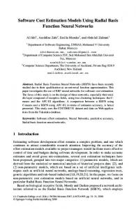
Now, to obtain we define the residual functions by substituting Eqs. (1.4)-(2.6) in Eq. (1.3) ˆ = κΦT (t)Ξ − (Iϑ ΦT (t)Ξ + u0 )(1 − I T (t)Ξ − u0 − I 2 ΦT (t)Ξ − u0 t). R(t) ϑ ϑ (2.7) come from The set of equations for obtaining the coefficients {ξi }N i=1 equalizing Eq. (2.6) to zero at N interpolate nodes {ti }N from tj = j=1 j ρ L( N ) , j = 1, 2, · · · , N where L is a last interpolate node and ρ is a arbitrary parameter. ˆ j ) = 0, j = 1, 2, · · · , N. R(t (2.8) 3. Application We applied the method presented in this paper to examine the mathematical structure of u(t). Table (2) shows the maximum of u(x) for some κ and u0 = 0.1 by using in comparison with exact solution and ADM solution by Wazwaz [3]. The resulting graph of Eq. (1.3) is shown in Fig. (1). Table 2.

A comparison of ADM[3] and the present method with exact values for umax . κ 0.02 0.04 0.1 0.2 0.5

umax 0.9234271 0.8737199 0.7697414 0.6590503 0.4851902

rω 1 1 1 2 2

ρ 1.766000 1.780000 1.811000 1.032770 1.114035

N 15 18 18 18 27

ICSRBF 0.92342716 0.8737193 0.7697414 0.6590493 0.4851903

ADM 0.9234270 0.8612401 0.7651130 0.6579123 0.4852823

The local support domain rω and arbitrary parameter ρ must be specified by the user.An important unsolved problem is to find a approach to determine the optimal size of rω [18]. The accuracy of these CSRBF depends on the choice of rω and ρ. By the meaning of residual function in case of Eq. (2.6), we try to minimize ∥R(t)∥2 by choosing good rω and ρ parameters. We define ∥R(t)∥2 as ∫ L m L∑ L L 2 ∥R(t)∥ = R2 (t)dt ≃ ωj R2 ( sj + ), (3.1) 2 2 2 0 j=0

84

PARAND , HEMAMI

Figure 1. Plot of approximate solutions of Eq. (1.3) for u0 = 0.1 and κ = 0.02, 0.04, 0.1, 0.2, 0.5. Table 3. Minimum value of ∥Res∥2 which is obtained with rω and ρ for ICSRBF. κ ∥Res∥2 -ICSRBF 0.5 2.11e − 08 0.2 2.87e − 07 0.1 1.34e − 07 0.04 7.86e − 05 0.02 4.41e − 05 were ωj =

L (1 −

d s2j )( dx Pm+1 (s)|s=sj )2

, j = 0, 1, · · · , m, Pm+1 (sj ) = 0, j = 0, 1, · · · , m,

Pm+1 (x) is (m + 1)th-order Legendre polynomial. Table (3) show the minimum of ∥R(t)∥2 which is obtained with local support domain rω and arbitrary parameter ρ . 4. Conclusion A method has been presented for solving Volterras population model which is an integro-ordinary differential equation, based on the compactly supported radial basis functions approximation. In this work, we applied two common ICSRBF methods on the Volterras population

ICSRBF FOR VOLTERRAS POPULATION MODEL

85

model without converting it to an ordinary differential equation. We used W endland3,5 function. This function are proposed to provide an effective but simple way to improve the convergence of the solution by collocation method. As appeared from the Figures, we have shown that, c when the constant κ = ab is small, this type of population is relatively insensitive to toxins, and when c = ab is large, population of this type are extremely sensitive to toxins. Additionally, through the comparison with ADM, we have showed that the ICSRBF approach have good reliability and efficiency.

5. References References [1] F. Scudo , Vito Volterra and theoretical ecology, Theor Popul Biol 2 (1971), 1–23. [2] K. TeBeest, Numerical and analytical solutions of Volterras population model, SIAM Rev 39 (1997),484-493. [3] A. M. Wazwaz, Analytical approximations and Pad approximants for Volterras population model, Appl Math Comput 100 (1999),13–25. [4] R. Small, Population growth in a closed system, SIAM Rev 25 (1983) 93–95. [5] K. Al-Khaled, Numerical approximations for population growth models, Appl Math Comput 160 (2005) 865–873. [6] K. Parand , A. Rezaei, A. Taghavi, Numerical approximations for population growth model by Rational Chebyshev and Hermite functions collocation approach: a comparison., Math Methods Appl Sci 33 (2010) 2076–2086. [7] M. Ramezani, M. Razzaghi, M. Dehghan, Composite spectral functions for solving Volterras population model, Chaos Soliton Fract 34 (2007) 588–593. [8] K. Parand, S. Abbasbandy, S. Kazem, J. A. Rad, A novel application of radial basis functions for solving a model of first-order integro-ordinary differential equation, Commun Nonlinear Sci Numer Simulat 16 (2011) 4250–4258. [9] HR. Marzban, S. Hoseini, M. Razzaghi, Solution of Volterras population model via block-pulse functions and Lagrange-interpolating polynomials, Math Methods Appl Sci 32 (2009) 127–134. [10] K. Parand, Z. Delafkar, N. Pakniat, MK. Haji Collocation method using Sinc and Rational Legendre functions for solving Volterras population model, Commun Nonlinear Sci Numer Simul 16 (2011) 1811–1819. [11] S. Momani, R. Qaralleh, N. Pakniat, MK. Haji, Numerical approximations and Pad approximants for a fractional population growth model, Appl Math Model 31 (2007) 1907–1914. [12] H. Xu, Analytical approximations for a population growth model with fractional order, Commun Nonlinear Sci Numer Simul 14 (2009) 1978–1983. [13] J. A. Rad, K. Parand, L. V. Ballestra Pricing European and American options by radial basis point interpolation, Appl Math Comput 251 (2015) 363–377. [14] J. A. Rad, S. Kazem, K. Parand Optimal control of a parabolic distributed parameter system via radial basis functions, Commun Nonlinear Sci Numer Simul 19 (2014) 2559–2567.

86

PARAND , HEMAMI

[15] S. Kazem, J. A. Rad, K. Parand, M. Shaban, H. Saberi The numerical study on the unsteady flow of gas in a semi-infinite porous medium using an RBF collocation method, Int J Comp Math 89 (2012) 2240–2258. [16] S. Kazem, J. A. Rad, K. Parand, A meshless method on non-Fickian flows with mixing length growth in porous media based on radial basis functions: A comparative study, Comp Math Applic 64 (2012) 399–412. [17] M. D. Buhmann, Radial basis functions: theory and implementations, New York: Cambridge University Press (2004). [18] S. M. Wong, Y. C. Hon, M. A. Golberg , Compactly supported radial basis function for shallow water equations, Appl Math Comput 127 (2002) 79–101. [19] H. Wendland, Piecewise polynomial, positive definite and compactly supported radial functions of minimal degree, Adv Comput Math 4 (1995) 389–396. [20] G. E. Fasshauer, Meshfree Approximation Methods With Matlab, World Scientific Publishing Co. (1995) Pte, Ltd 4 389–396. [21] G. E. Fasshauer, On smoothing for multilevel approximation with radial basis functions, An approximation theory IX, Vol. II: Coputational Aspects, CharlesK. Chui and L. L. Schumakher., Vanderbilt University Press. (1999) Pte, Ltd 4 389– 396. [22] Z. Wu, Compactly supported positive definite radial functions, Adv Comput Math 4 283–292. [23] M. D. Buhmann, A NEW CLASS OF RADIAL BASIS FUNCTIONS WITH COMPACT SUPPORT, Math Comput 70 307–318. .