Compact Object Recognition Using Energy-Function-Based Optimization

770

IEEE TRANSACTIONS ON PATTERN ANALYSIS AND MACHINE INTELLIGENCE, VOL. 14,N0. 7,JULY 1992

Correspondence Compact Object Recognition Using Energy-Function-Based Optimization

The automated version of Fua and Hansen’s method seems to break down the process into several stages that are pipelined together. This type of piecemeal approach is an inefficient utilization of the N. S. Friedland and Azriel Rosenfeld available information. The data processing theorem [4], which is a well-known result in information theory, states that the more “black boxes” that are strung together in sequence, the poorer the quality of Abstract-This paper describes a method of recognizing objects whose the information becomes, unless strict coding criteria are met. Since contours can be represented in smoothly varying polar coordinate form. the highest level, and thus most important, decisions are usually made Both low- and high-level information about the object (contour smoothat the last “box,” the performance of a segmented system could be ness and edge sharpness at the low level and contour shape at the high level) are incorporated into a single energy function that defines a l-D, problematic. Backtracking can improve this somewhat, but it requires cyclic, Markov random field (1DCMRF’). This 1DCMFW is based on a the ability to determine if and where an error has been made. polar coordinate object representation whose center can be initialized at In this paper, we present an energy function minimization method any location within the object. The recognition process is based on energy of recognizing a class of objects that we call compact objects. A function minimization, which is implemented by simulated annealing. compact object is a star-shaped object [5], i.e., an object whose entire Index Terms-Markov random field, object detection, object recognicontour is visible from an interior point. In addition, in a compact tion, simulated annealing. object, we require that the radii are not highly variable relative to the size of the object. Such an object’s contour can be represented in I. INTRODUCTION polar form by a smoothly varying radius function. We incorporate the recognition criteria into an energy function The idea of formulating an object recognition problem as an (EF) that equivalently defines a Markov random field (MRF). These optimization problem is of interest because a large family of powerful optimization techniques can be utilized. This paper describes a criteria consist of contour smoothness and edge sharpness at what we call the “low level,” which primarily works on localized regions method of recognizing objects by energy function minimization. The concept of using energy function minimization to find smooth of the raw image data; and contour shape at the “high level,” which compares the entire contour to a set of known geometrical shapes. contours in an image has been explored in the past. Kass et al. [l] presented a class of active contour models called “snakes,” which are Thus, local and global criteria are combined in the same EF, which basically controlled continuity splines. The energy function consisted results in a single-stage recognition process. The optimization method of a linear combination of three components that attract the snake used is simulated annealing, which provides the means of driving the to lines, edges and, terminations. Although the authors do discuss energy to its lowest value and, hence, leads to an MRF state with incorporation of high-level knowledge, it is not obvious how this the highest probability. Our approach differs from those reviewed above in several imporcan be done in the case of global geometrical properties. It is also unclear how much the success of this method is dependent tant respects: on human initialization and interaction. Since energy values result 1) It represents the compact object’s contour in polar form. The from integrating along the entire snake, every part of the solution center of the polar representation can initially be anywhere is dependent on the entire configuration. From a computational inside the contour. The position of the center can then be point of view, this is an expensive procedure that employs matrix iteratively shifted toward the centroid of the contour to provide computations that become more cumbersome as the complexity of the best “view” of the contour. the energy function increases. 2) It operates on raw data and incorporates both local information Fua and Hansen [2], [3] used an approach based on information (contour smoothness and edge sharpness) and global infortheory to perform region extraction. This approach seems superior to mation (object shape) simultaneously during the optimization, the snakes methods because it has the ability to incorporate global resulting in an information-efficient single-stage recognition geometric requirements in its optimization process. It is, however, process. limited in its ability to handle real images. A noise model must 3) These types of information are given weights that change be assumed in order to deal with the difficult task of determining during the course of the optimization. conditional probabilities. It is also assumed that the regions in 4) No noise model assumptions are needed. Conditional probabilquestion are primarily homogeneous in gray level; departures from ities are not calculated explicitly. this assumption, which occurs frequently in real images, will lead to 5) The optimization method is highly parallelizable since it is poor performance. Finally, it is assumed that the region shapes are based on an MRF. highly uncorrelated; this is a very severe constraint that may be too 6) The algorithm outputs a measure of confidence in the object’s limiting in the real world. classification. Thus, unknown objects can be identified as such. 7) A stopping criterion can be imposed once a desired degree of ManuscriptreceivedDecember20, 1989; revisedJuly 18, 1991. This work confidence has been obtained. was supported by the Defense Advanced ResearchProjectsAgency, under ARPA Order 6989, and by the U.S. Army Engineer Topographic Laboratories The basis for the polar representation was developed in an earlier under contract DACA76-89-C-0019. Recommended for acceptance by Assopaper by Friedland and Adam [6] in which an energy function was ciate Editor R. Woodham. used to detect and delineate cavity boundaries in noisy ultrasonic The authors are with the Center for Automation Research, University 01 images. The use of high-level information and the ability to iteratively Maryland, College Park, MD 20742-3411. shift the polar representation’s center are new; we have found that IEEE Log Number 9104991. 0162-8828/92$03.000 1992 IEEE

IEEE TRANSACTIONS ON PATTERN ANALYSIS AND MACHINE INTELLIGENCE, VOL. 14, NO. 7, JULY 1992

they greatly increase the power of this approach. Section II of this paper presents a description of the MRF representation as it relates to our problem. Section III describes our EF, Section IV discusses our choice of optimization technique, Section V presents experimental results, and Section VI contains a discussion.

771

2. Using a 1DCMRF simplifies the segmentation problems that are encountered when a regionwise homogeneous MRF is assumed. Due to the lower dimensionality of the lDCMRF, this segmentation involves only checking for arcwise smoothness of the object’s boundary. C. The Iterative Center Shifts

II. THE POLARMRF REPRESENTATION A. Markov Random Fields and Gibbs Distributions In their 1984 article, Geman and Geman [7] showed how statespace type optimization algorithms that had been developed for statistical physics (see Metropolis et al. [8] and Kirkpatrick et al. [9]) could be used for restoration of degraded images. They showed that an EF that satisfied certain rather simple conditions defined a Gibbs distribution over the state space. They also demonstrated that the existence of the Gibbs distribution is equivalent to the existence of a MRF. It is this property that makes the Gibbs distribution/EF approach such a powerful tool because by defining a proper EF, a consistent conditional probability environment is established. Thus, the difficulty of defining conditional probabilities is overcome, and an extremely versatile and easy to implement method is established. B. The 1-D Cyclic Markov Random Field The difficulties that have arisen in past attempts to apply MRF methods to images have been due to two major causes: 1. It is common practice to define the MRF sites as coinciding with the pixels of the image, as in [7]. Even for a lowresolution image of size 64 x 64, the resultant processing time is enormous. 2. The common assumption of homogeneity in the MRF defined by the pixel gray-level values is unwarranted. Homogeneity can be assumed for local regions, but this localization, being data dependent, is not simple to implement, and boundary conditions must be satisfied between neighboring areas. These problems have led us to propose a different approach to applying MRF methods to the object recognition problem. We use MRF methods at the level of geometric region representation rather than working at the pixel array level. Specifically, we define a 1-D cyclic MRF (1DCMRF) on a polar-coordinate (R. 0) representation of the region relative to a given center. Thus, each radius becomes a random variable and a site in the 1DCMRF. Let R = (~1.. . T,, } be a vector of discrete random variables rl, which represent distances from a given center, and let d = { ri = dl.l.2 = &!.“‘.I-, =&s,, } represent a possible configuration of that vector. Here, d’r is an I’, sample point and d E Q, where f2 is the MRF’s sample space. The 1DCMRF is thus defined as follows:

Our implementation of the 1DCMRF allows the center (from which the radii emanate) to shift. At given intervals in the optimization process, we calculate the centroid of the current 1DCMRF configuration .J. This centroid becomes the new center. Using this new center, the 1DCMRF is regenerated; d is transformed to 2 defined relative to the new center. This ability of the algorithm to shift its origin eliminates the need to choosing a “good” center initially. Our experimental results demonstrate the stability of this center shifting process. From different starting points, the center will stabilize in the same spatial location for a given object. III. THE ENERGY FUNCTION A. General Formulation In the Ising model [lo], the energy function depicts energy relationships between site spins in a solid lattice. A magnetic dipole-dipole interaction field energy relationship exists between neighboring sites on the lattice (local operator), whereas an external field affects each individual site spin regardless of the neighboring values (global operator). Geman and Geman [7] demonstrated that the interaction and external field concept of the Ising model can be replaced with a pseudo-physical environment in which the field relationships are artificially constructed. This new EF concept still generates a legal Gibbs distribution and, equivalently, a legal MRF. The importance of this is that now, all the mathematical tools that were developed to study the original physical process can be implemented for the pseudo-physical system defined by the new EF. The general formulation of our energy function is

VI,ER

vr, ER

where I r is called a potential function. The terms of the first sum are called external field elements of IT, and those of the second sum are called interactive elements. Equation (3) allows complex criteria to be incorporated into the same EF. The potential functions Ii L1 and Ii (,J JEU, 1 can be linear combinations of subfunctions [6], where each incorporates a separate criterion. B. Application to Object Recognition

Our approach to compact object recognition consists of three main stages: and 1. Detection: detecting a candidate “object center” in the image. This center can be anywhere inside the object. P(r, = bull1 rJ = di’): j #i)=P(r,=~~lr,=~,:jES,) (2) 2. Representation: representing the candidate object in polar coordinate form, relative to the center, and identifying the vi E {1.2:... n} andVd E f2 location of its contour along each radius where N, is a neighborhood of P,. For simplicity, we take S, to be 3. Matching: comparing the polar coordinate representation of {i - 1. i + l}, and we use equispaced radii at angular intervals of the object with a set of stored representations. &9 = %. Since we are dealing with a closed contour, r,>+i = ri, We have incorporated the second and third stages into the EF. This has and the neighborhoods are defined modulo II. the advantage that all known information about the possible objects Using this 1DCMRF based on a geometric object representation is utilized simultaneously. has two major advantages over using MRF’s on pixel arrays: We combine the second and third stages by using what we call 1. The MRF is not a 2-D pixel array but a 1-D array of size 11. an adaptive multilevel energy function (AMEF). This EF consists of two processing levels: a low level (LL), consisting of local operators This provides an immense computational advantage. P(R=

J)>

0

Vd E fl

(1)

IEEE TRANSACTIONS ON PATTERN ANALYSIS AND MACHINE INTELLIGENCE, VOL. 14, NO. 7, JULY 1992

772

that examine information at the pixel level and generate a radial representation of the object’s outline, and a high level (HL), which matches the LL radial configuration to a library of existing object configurations. Symbolically n I-(;) = 11-l x ELI>(~) + Ii, x EIIL(;) (4) where H-1. Ii-2 are the adaptive weight functions, and E~,L. EIJL are the LL and HL elements, respectively. d E R is the radial configuration space. The goal is to find a contour that gives a best fit to the pixel data from the LL process while the object classification is a “bonus,” which is gained when the HL participates in the fitting. The weight function II-2 in (4) varies in the course of the optimization and is determined by examining the behavior of the system. The recognition process is initialized by selecting a center location somewhere within a candidate region that the detection process has selected as a possible location of an object. Next, a 1DCMRF R is established by defining n equispaced random radii emanating from this center. A random initial guess configuration R = iv’0 is then assigned to the 1DCMRF so that an initial Gibbs density, which corresponds to the probability density of each site r1 E R, can be calculated (see [6]). Then, the optimization process is allowed to begin. After a given number of sweeps over R, R’s center is shifted to the centroid of d. The resulting configuration R = -C is used to select an object from the data set G ”bJ.B, which provides the best match to it. The selected object will subsequently be used in the EF. At this time, the Gibbs densities are also redetermined. A priori information about object size can define an upper bound rCrf for the radii. This will reduce the amount of computation needed to update the local Gibbs densities. The above cycle is allowed to continue until either a compatible object has been found in the data set G ”hJ,” or an upper bound has been reached on the number of optimization iterations. It is important to stress that throughout the process, we are using the same EF system, although the EF itself is undergoing changes. A conservative but time-consuming method of handling the detection step would be to subdivide the entire image into possibly overlapping regions and to initialize the recognition method in each region. A region would be eliminated if the algorithm failed to detect a relevant object. This approach is the most likely to avoid major detection errors. Its cost may not be prohibitive if the regions can be independently processed in parallel. In the following subsections, we will elaborate on the LL and HL processes and the corresponding parts of the energy function. C. The Low-Level Process The low-level component of the energy function controls contour smoothness and edge sharpness. This is done by examining very localized regions along the contour. Edge sharpness is tested at each radius individually, whereas contour smoothness is achieved by comparing each radius value to its nearest neighbors. This combined process results in contour configurations that are free of spurious edges due to high-frequency noise; at the same time, it maintains high-frequency information about the contour that would have been lost in a post-edge-detection smoothing. The contour smoothness operator is 0 s,,~oothnrs.~~rr Je IrL - ” ’ j.yl.;’ + I”+‘)’

(5)

where r,-1. rc. r,+i are radii/site values, and rtzt is a constant representative of the window size used. The edge sharpness operator is a gray-level step detector

where x(. ) is the local gray-level value at the given radius/site value, and J1 is the half size of the step filter. These two operators are combined linearly into the LL portion of the EF: n

where n 1. oa are constants, and M.44GR.41is the gray-level quantization. The low-level process is also used to extract information about the contrast between the target and the background. This is done by examining the average edge detector value (6) for the radial configuration. This value can be used to determine what the contrast of the edges should be. Edges with the improper contrast are overlooked, allowing the LL to concentrate on relevant edges only. This LL portion of the EF is assigned a constant weight 11-i throughout the optimization. Its initial purpose is to construct an initial approximation of the object’s contour; later, when the HL process becomes more dominant, the LL portion ensures that the HL does not create “artifacts” that are not corroborated by the image data. D. The High-Level Process The HL process consists of the following steps: At every kth step (for some preselected k) of the iterative optimization process, we attempt to match the current radial configuration R = J to a set of stored radial contour representations Gob’,‘, where obj is the object number, and 0 is the object’s orientation. These radial representations are stored in normalized form, i.e., they are divided by the mean of their values and are resealed to R’s mean size for the matching process. In the matching process, the match error is defined by

where r,,,,,,, is the mean value of the current radial configuration R = b’. GobJ.’ IS selected as the contour having the lowest Er value. This error value can be compared with a cutoff threshold to establish a halting criterion for the algorithm. It can also indicate the quality of match attained. Once a data representation contour G ”h’.0 has been selected, a penalty is assigned to R configurations that greatly deviate from it. This is accomplished in the EF’s high-level component as follows:

where r, is the local radius value, Gpb’.’ is the ith radius value of configuration G ”bZ,“, and riZt is a constant representative of the window size. During the course of the optimization, several objects (possibly in several orientations) may be selected. To prevent the selected objects from unduly influencing the low-level, an adaptive weight is used for the high-level component of the EF. The weight Ii, assigned to EHL is inversely dependent on Er”“.“: A Ti:~=a:s x (1 - EI obj.0,, (10) The smaller the error, the larger 11, becomes relative to II;. This is desirable since it implies that the high level becomes more active as its confidence in its match increases. Since all objects in the data set are comuact. all of them will hem the low level attain contour smoothness

IEEE TRANSACTIONS ON PATTERN ANALYSIS AND MACHINE INTELLIGENCE, VOL. 14,NO. 7,JULY 1992

in the initial stages of the optimization. As the optimization reaches its conclusion, i.e., the global minimum of the energy, and the radial representation grows closer to the actual contour in the image, I,IrZ will grow (provided an appropriate object representation appears in G”‘b’.B). As a result, the high level will become more dominant and speed up the final convergence of the optimization. To summarize, the high level is an active participant in the EF and not merely a postprocess. This gives the system top-down qualities-a very important point. In addition, by providing a limit to the number of iterations performed, the high level allows the detection result of “don’t know” to be obtained. E. A Word of Caution No general theoretical basis exists for defining an accurate energy description of a given system. Such a description would result in a physically significant optimum and fully utilize the power of the EF approach. Since this theory, in the general case, is lacking, the EF is defined heuristically. It was demonstrated in [6] that although the EF used was suboptimal, the results attained were very good. To summarize this section, the attractiveness of using an EF approach to a given problem is determined by the ability to describe the system using (3) and its modifications. In some cases, this is a trivial problem; in others, in order to achieve a practical implementation, the dimensionality of the MRF must be reduced through a transformation of some kind. The main advantages of using an EF are that the restrictions that (3) imposes are not great, although it allows a high degree of design freedom to integrate a lot of information into the system. The main disadvantage is the lack of theoretical tools for assessing the quality of the selected EF; this is done by an empirical process of trial and error.

773

In Geman and Geman [7], the optimization was performed using simulated annealing, which is often a very time-consuming algorithm and does not ensure convergence to a global minimum in a finite time. Our own experiments in [6] showed that the algorithm converged well for very noisy data and required a relatively short convergence time due to the reduced dimension of the MRF employed. B. Parallelism In Section II, we pointed out that MRF’s have the property of limited statistical dependence between a given site r, and the rest of the field. This property makes MRF’s very attractive from a parallel implementation point of view. Each site can be assigned a processor whose operation is independent of most of the other sites. Only the defined neighborhood supplies the processor with an updated energy configuration. This type of implementation is not straightforward. Margalit [12] showed that the sets of MRF sites processed at a given time must be separated from one another in order to achieve reasonable convergence. This restriction can be imposed by dividing the field into subarrays whose points are the desired distance apart and applying parallel processing to one subarray at a time. The MRF implemented in our system shares the same neighborhood relationship at each site because the interactive components (5) are identical in each one. Thus, all the parallel processors can be built identically with identical connectivity to neighboring processors. Hence, this algorithm lends itself naturally to parallel implementation, with all its obvious advantages.

V. EXPERIMENTAL RESULTS IV. THE OPTIMIZATIONPROCESS

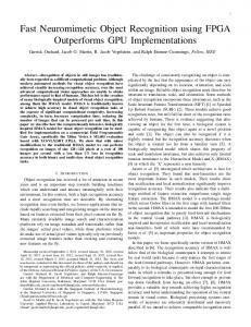
In this section, we demonstrate some of the characteristics of our approach. The data used are images obtained by a forward-looking A. Method infra-red (FLIR) sensor. These images contain a high level of noise Once the MRF is defined by the EF, local perturbation techniques that originates in both the medium and the sensor [13]. It thus cannot can be used to bring the MRF to its highest probability state and, be assumed to be strictly additive in nature. equivalently, the EF to its global minimum. The ability to restrict the The results shown in this section are grouped into ten figures. process to a limited neighborhood is due to the property of the MRF The state space configuration is shown in these figures at every tenth defined in (2), namely, that the probability of site TVattaining value UJ, iteration. The upper left picture in each figure shows the initial image given the entire MRF configuration depends only on a neighborhood window (85 by 85 pixels); the initial location of the center is marked of T,. (This property will become very important when we discuss with a +. The other pictures in each figure have had their gray scales parallel implementations in the next subsection.) compressed from [0,255] to [60,195] for display purposes. A white An example of how local perturbation is used here will now be contour (gray level 255) is superimposed on each picture; it shows presented. Suppose UQ E R is a given configuration of our MRF R, the radial configuration of the 1DCMRF. When the HL process is with the local site attaining the value T, = wt. The corresponding EF active, a black contour (gray level 0) is also superimposed; it shows value is I:(wl ). Now, a new value P, = & is selected for the site. the best matching library object scaled by T,,,,,, and rotated by 0. The resulting state space configuration is LJ~, which in turn yields For cases in which the HL has been shut down, the black contours U (dT). The optimization algorithm can now examine are not displayed. Associated with each iteration are two to four numbers. The a, AiT=ti (wz) - V(4). (11) number in the top left corner designates the current best matching A hill-climbing-type algorithm would accept .rZ = S, values that library object; the objects are three tanks, a truck, a bmp, and a jeep. The number in the upper right corner represents the degree of match render AI’ < 0, whereas stochastic methods may accept, with 1 - Er between the best matching library object and the 1DCMRF. certain probabilities, j, values for any value of AL’. The type These numbers do not appear when the high level has been shut off. of method employed depends greatly on our a priori knowledge The lower numbers represent the contrast between the object and of the EF’s behavior. For example, if we know that the EF is smooth and unimodal, a simple hill-climbing algorithm suffices. The the background (on the left) and the iteration number (on the right). In computational cost of such an algorithm is low, and its convergence order to determine the contrast, at every tenth iteration, the algorithm computes the average edge strength (6). If the absolute value of this is rapid. On the other hand, if the EF is smooth and complex, i.e., multimodal, simulated annealing can be utilized. There are also strength is high (2 10, in our experiments), the algorithm decides on the sign of the contrast (positive for dark objects on light backgrounds classes of functions for which the solution of the minimization and negative for light objects on dark backgrounds), and during the problem is intractable, for example, the golf course problem [ll]. This case can sometimes be avoided by making I:(uJ) as smooth as next ten iterations, the edge-detection process is set to detect only edges with the appropriate sign of contrast. possible with minimal high gradient areas.

Fig. 3.

IEEE TRANSACXIONS ON PATTERN ANALYSIS AND MACHINE INTELLIGENCE,VOL. 14,NO. 7,JULY 1992

177

[2] P. Fua and A. J. Hanson, “Objective functions for feature discrimination: Theory,” in Proc. DARPA Image Understanding Workshop, 1989, pp. 443460. [3] -, “Objective functions for feature discrimination: Applications to semiautomated and automated feature extraction,” in Proc. DARPA Image Understanding Workshop, 1989, pp. 676-694. [4] R. G. Gallager, Information Theory and Reliable Communication. New York: Wiley, 1972, p. 80. [5] A. Rosenfeld and A. C. Kak, Digital Picture Processing. New York: Academic, 1982, p. 270, vol. 2. [6] N. Friedland and D. Adam, “Automatic cavity boundary detection from sequential ultrasound images using. simulated annealing,” IEEE Trans. Med. Imaging, vol. 8, pp.-344-35T3, 1989. [7] S. Geman and D. Geman, “Stochastic relaxation, Gibbs distribution, and the Bayesian restoration of images,” IEEE Trans. Patt. Anal. Machine Zntell., vol. PAMI-6, pp. 721-741, 1984. [S] N. Metropolis, A. W. Rosenbluth, M. N. Rosenbluth, A. H. Teller, and E. Teller, “Equation of state calculations by fast computing machines,” J. Chem. Phys., vol. 21, pp. 1087-1091, 1953. [91 S. Kirkpatrick, C. D. Gelatt Jr., and M. P. Vecchi, “Optimization by simulated annealing,” IBM Res. Rep. RC 9355, 1982. [lOI E. lsing, Zeitschrift Physik, vol. 31, p. 253, 1925; see, for example, C. J. Thompson, Mathematical Statistical Mechanics. New York: Macmillan, 1972. 1111E. B. Baum, “Graph orthogonalization,” to be published in Discrete Mathematics. [121A. Margalit, “A parallel algorithm to generate a Markov random field image on a SIMD hypercube machine,” CS-TR-2050, Cent. Automat. Res., Univ. of Maryland, College Park, 1988. [I31 G. H. Kornfeld, ‘Digital similation of precise sensor degradation including nonlinearities and shift variance,” in Proc. SPZE Infrared Image Processing Enhancement, vol. 781, pp. 63-70, 1987.

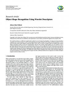
Fig. 10.

On Achievable Accuracy in Edge Localization

Results using LL and HL in which the object is not in the model database.

Ramakrishna

Kakarala

and Alfred

0. Hero

TABLE I ALGORITHM PARAMETERS Definition

Value

low-level weight function

1.0

upper bound on radii

42

edge filter half length

5

smoothnesss operator constant

0.4

edge operator constant

1.0

14-2 coefficient

0.1

matching convergence threshold

90%

maximum grey-level value

255

dimension of 1DCMRF (number of radii)

32

Abstract-Edge localization occurs when an edge detector determines the location of an edge in an image. In this note, we use statistical parameter estimation techniques to derive bounds on achievable accuracy in edge localization. These bounds, known as the Cramer-Rao bounds, reveal the effect on localization of factors such as signal-to-noise ratio (SNR), extent of edge observed, scale of smoothing filter, and a priori uncertainty about edge intensity. By using continuous values for both image coordinates and intensity, we focus on the effect of these factors prior to sampling and quantization. We analyze the Canny algorithm and show that for high SNR, its mean squared error is only a factor of two higher than the lower limit established by the Cramer-Rao bound. Although this is very good, we show that for high SNR, the maximum-likelihood estimator, which is also derived here, virtually achieves the lower bound. Index Terms-Cramer-Rao lower bound, edge detection, edge localization, maximum-likelihood estimator, mean squared error.

ACKNOWLEDGMENT The authors would like to thank B. Kamgar-Parsi comments and suggestions.

for his helpful

REFERENCES [l]

M. Kass, A. Witkin, and D. Terzopoulos, “Snakes: Active contour models,” Int. J. Cornput. Vision, vol. 1, pp. 321-331, 1988.

0162-8828/92$03.00

Manuscript received May 23, 1990; revised August 5, 1991. R. Kakarala is with the Department of Mathematics, University of California, Irvine, CA 92717. A. 0. Hero is with the Department of Electrical Engineering and Computer Science, University of Michigan, Ann Arbor, MI 48019-2122. IEEE Log Number 9107545.

0 1992 IEEE