Comparing clustering methods for market segmentation: A simulation study Received (in revised form): 29th July, 2016
Chad Vidden has a PhD in Applied Mathematics, with expertise in computational mathematics, data science and machine learning. He is currently an assistant professor at the University of Wisconsin – La Crosse, where he leads a data science and mathematical modelling research group that collaborates with local companies. 1009 Cowley Hall, University of Wisconsin – La Crosse, La Crosse, WI 54601, USA Tel: +608 785 5214; E-mail:
[email protected]
Marco Vriens has a PhD in Marketing Analytics, and is a expert in applied analytics. He is currently Chief Research Officer at Ipsos and faculty member at the University of Wisconsin – La Crosse. He has led analytics teams for Microsoft, GE and supplier firms. Marco is the author of three books: The Insights Advantage: Knowing How to Win (2012), Handbook of Marketing Research (2006) and Conjoint Analysis in Marketing (1995). Marco has been published in academic and industry journals and has won several best paper awards including the David K. Hardin Award. Tel: +608 518 8399; E-mail:
[email protected]
Song Chen has a PhD in Applied Mathematics and is an assistant professor at University of Wisconsin – La Crosse. He conducts research in scientific computing and data mining with applications in fields such as marketing. He is director of the data science group at University of Wisconsin – La Crosse and actively leads undergraduate collaborative projects with local industry. 1007 Cowley Hall, University of Wisconsin – La Crosse, La Crosse, WI 54601, USA Tel: +608 785 8826; E-mail:
[email protected]
Abstract This paper compares clustering methods on simulated data sets with different characteristics, such as degree of variance, whether there are overlaps between segments, the nature of the true clusters, and the absence/presence of categorical variables. Specifically, the paper compares K-means with latent class and ensemble analysis. The authors’ findings show that latent class analysis performs best in most cases, both in its ability to recover the true cluster members and in its ability to identify the correct number of clusters. Ensemble methods perform second best. K-means performs reasonably well with continuous variables. The current authors also tested the core member approach that can be applied on top of any clustering method, and found that it improved the identification of the correct cluster members. KEYWORDS: market segmentation, cluster analysis, ensemble analysis, latent class analysis, simulation
© Henry Stewart Publications 2054-7544 (2016) Vol. 2, 3 225–238 Applied Marketing Analytics
225
Vidden, Vriens and Chen
INTRODUCTION Market segmentation is an essential and popular marketing tool that can offer firms insights for growth (ie new product ideas) and efficiency (ie better marketing communication, better focus on the right audience). The risk that a segmentation project may fail is high, though. A Harvard Business paper1 claimed that in the USA, 85 per cent of 30,000 new product launches failed because of poor market segmentation. Both business and analytical considerations play a big role throughout the segmentation development process. Analytics is important, because it is needed to discover whether or not consumers are heterogeneous in a discrete way based on data on a number of variables: eg behaviours, attitudinal statements, life-style variables, values, needs, etc. The choice of variables in and of itself is an important step mainly driven by business considerations. For example, if product development is a key objective, the firm may want to ask about unmet needs and behaviours. Once the firm has data on a set of variables, clustering methods are applied to determine whether consumers differ on these variables. Clustering and related methods have long been the workhorses for commercial market segmentation.2 In practice, the most often used methods, K-means and hierarchical clustering, have several unappealing features3,4 and can be used only for continuous variables (eg ratio or interval scaled variables) but not for categorical variables.5,6 Several developments are offering an alternative to these popular methods. First, latent class analysis methods have become somewhat popular, and represent a statistical model-based alternative to clustering. This approach can handle categorical data. Secondly, the k-modes approach, an extension of the K-means approach, has been proposed to handle categorical or mixed variable type data.7–9 Thirdly, ensemble methods10 have become available. They combine multiple
226
cluster solutions to arrive at a new, and hopefully better, solution. The notion is that by combining over multiple solutions one can increase the stability and quality of the cluster solution. Ensemble methods have been shown to produce more accurate solutions than K-means or hierarchical clustering algorithms.11,12 For example, a user might generate a number of K-means solutions, a number of hierarchical cluster solutions and then combine these solutions into a new ensemble solution. The field of ensemble analysis is an emerging field, and little is known about the precise conditions that will lead to a better final solution. Fourthly, the identification and use of so-called core-cluster members13 has gained some traction in commercial applications. The idea here is that one can increase the validity of the solution by using only those classified members for which we can claim segment membership with confidence: ie we distinguish between members that are close to the centre of the clusters (segments) and those more at the fringe of a given cluster. The use of core members has two steps: (1) we generate a cluster solution; (2) we determine which members are core and which are not, and only use the core members to interpret the cluster solutions. The main motivation is to ignore uncertain classification and focus on certainty. We distinguish between members who have a high likelihood of belonging to the cluster and those who are at the fringe and have a lower probability of belonging to the cluster in which they were classified. Fifthly, SPSS14,15 have introduced a new approach referred to as ‘twostep cluster analysis’. It has the ability to handle mixed variable data and automatically selects an optimal number of clusters. It can be viewed as a combination of K-means and hierarchical clustering. SPSS twostep starts with a fast pre-clustering (K-means-like) approach to create sub-clusters and then in a second stage uses the hierarchical approach.16
Applied Marketing Analytics Vol. 2, 3 225–238 © Henry Stewart Publications 2054-7544 (2016)
Comparing clustering methods for market segmentation
There are several pieces of evidence missing in the literature that we believe would be good for practitioners to know: 1. There have been, to our knowledge, no direct comparisons between ensemble methods and latent class methods. Knowing this is important, as ensemble methods involve an extra step in the clustering process. 2. Ensemble solutions can be created in various ways. In most cases we see K-means being used to create the ensemble. We would expect better results by using latent class analysis or K-modes given that the input data to an ensemble are a set of cluster solutions and hence the input data are categorical. 3. There are only a few papers that have made the comparison between K-means and latent class, so the body of evidence as to what works and when is still fairly thin. K-means and latent class were compared on simulated data with continuous variables only.17 The latent class model resulted in a misclassification rate of 1.3 per cent, whereas K-means resulted in a 5 per cent misclassification rate. Especially little is known about the relative performance of these methods in situations where we have a mix of continuous and categorical variables, and it is important to know if latent class truly works better in such cases. 4. The core paradigm can be applied on any clustering method, but in the studies where this approach worked well it was used only on K-means solutions in unpublished commercial studies. We do not know how the core-member approach performs across a variety of data situations and whether it would improve latent class or ensemble solutions. 5. There are two studies that have investigated SPSS twostep.5 A first study based on two continuous variables, and five clusters of equal size,18 found that SPSS twostep is able to recover the true segments with 100 per cent accuracy,
whereas K-means only achieves a success rate of 56 per cent. A second study included a mix of continuous and categorical variables.5 Some of their simulated segments were overlapping, as they considered these more realistic. SPSS twostep performs well in the case where all variables are continuous, consistent with the first study.18 When the segments were not well separated, the approach did poorly, unable to detect the correct number of segments. In the mixed variable data situations, SPSS twostep performed poorly as well. Given the popularity of SPSS it would be good to know whether or not the use of this approach is well justified or not. In this paper we investigate the five issues using simulated data sets. The methods are being evaluated on their ability to identify the correct number of segments, hit rates and reproducibility rates. SIMULATION STUDY Methods compared We compare the following methods: K-means (KM), SPSS twostep clustering, latent class analysis (LCA), K-means ensemble (KM-E), K-modes ensemble (KMO-E) and latent class ensemble (LCA-E). We also looked at how the use of core members would improve solutions using the cluster uncertainty approach.19 All approaches have been described in the literature and hence are not described here. We only summarise the specifics of how we implemented each approach. As mentioned in the beginning, most methods can be implemented in a variety of ways. To be able to interpret our results we briefly outline in the following how each method was run. Apart from the twostep approach, which is run within SPSS, all methods were implemented in the R programming language using existing R-modules. KM is
© Henry Stewart Publications 2054-7544 (2016) Vol. 2, 3 225–238 Applied Marketing Analytics
227
Vidden, Vriens and Chen
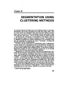
Figure 1: Visual illustration of using core segment membership
implemented through the kmeans R-routine included in the stat programming package. Latent class analysis is implemented using the R package mclust. Ensemble analysis was run by combining all LCA runs and the most reproducible KM runs via the indicator matrix method. This implementation is similar to the approach used by Sawtooth Software.12 Once combined, the (simulated) respondents were classified via KM or LCA. We refer to these methods as KM ensemble (KM-E) and LCA ensemble (LCA-E). Note that this refers to the method used to build the ensemble and not to the input solutions that are combined in the ensemble analysis. In each ensemble implementation we combine a variety of KM and LCA solutions.20 To implement the core approach we calculated for every classified respondent, the distance to all cluster centers. Intuitively, members belong to the uncertainty core group if they lie close to one cluster centre and far from all others. To calculate for a member, find the distance to all other cluster centres. If the distance from the member’s assigned cluster centre is nearly the same as another cluster centre, this member is
228
uncertain and does not belong in the core. To assign the core group, we delete 20 per cent of members that are most uncertain in this way. Figure 1 illustrates visually the effects of looking at core segment members. Evaluation approaches We compare these methods on the following metrics. Hit rates: This is a direct comparison to the true cluster solution, which gives an objective way to gauge how the various approaches are performing relative to each other. Hit rates are calculated through the adjusted Rand index.21,22 In a commercial application we do not know the true clusters of course. In fact, we do not even know whether or not there are any clusters. Instead we use statistics that can help us to determine the optimal number of clusters. That is, statistical measurements are used to guide the choice of the correct number of clusters. The metrics that we use include the following. Reproducibility rates: For KM, KM-E, KMO-E and LCA-E, these are calculated
Applied Marketing Analytics Vol. 2, 3 225–238 © Henry Stewart Publications 2054-7544 (2016)
Comparing clustering methods for market segmentation
as in the Sawtooth’s CCA technical paper.23 For KM we calculated the reproducibility rate by replicating each cluster solution ten times using different initialisations (80 runs in total for each method). For a given number of clusters, all ten runs are compared to each other to determine how consistent they are. If the ten runs agree, then the reproducibility is high. For LCA we use a bootstrap approach so we can calculate reproducibility rates.24 The mclust module that is used to run LCA always produces the same result for a given cluster size, so we used bootstrapping (accomplished by random sampling of the original data set with replacement) as an alternative. These samples were appended to the original data set. For example, a data set of size 1,000 was sampled 1,000 times. Appending these samples to the original set gives a sample of size 2,000. LCA was then run on this data, and the results were kept only for the original 1,000 data points. This allows a way to produce ten distinct LCA clustering solutions for each cluster size 2–9, producing 80 total LCA runs and reproducibility rates are calculated as above. The GAP statistic: This statistic looks at the statistical difference between the clustering results and a completely random data set. A bigger difference indicates that the clustering result has a clearer statistical pattern. The GAP statistic outperforms many other approaches in estimating the number of clusters for KM.25 It also has the ability to identify one cluster solution, ie the situation where the data should not be clustered at all, but can only be used for numerical data. BIC (Bayesian Information Criterion)26: The BIC statistic is based on maximum likelihood estimate and adds a penalty term to prevent overfitting. Models with a lower BIC number indicate a better fit of the data. BIC was used only for the LCA results in the mixed variable case. Each of these metrics were calculated for a 2–9 cluster solution. The results were plotted and through visual inspection we
identified the most likely true segmentation solution. We used three summary statistics to compare the performance of the various methods on three practically relevant criteria: 1. 100 per cent success rate (SR100): This is the percentage of times across the six data sets that a method uniquely correctly identified the correct number of clusters. For example, Figure 2a shows the BIC values across the 2–9 cluster solutions. It clearly indicates only one cluster solution as the best cluster solution: the 3 cluster solution (because reproducibility is at the highest level there). 2. Practical success rate (PSR): In practice it is very common to investigate multiple cluster solutions and use other (non-statistical) criteria to select the optimal cluster solution for a firm such as managerial usefulness. See Figure 1b for an example (showing K-means reproducibility rates for the 2–9 K-means solutions). As this figure shows, several cluster solutions have more or less equal reproducibility levels and would be candidates for the best cluster solution as they both have higher reproducibility rates than other cluster solutions. One of these solutions is the true solution, and given that in a practical situation these will probably both be reviewed we refer to this as the practical success rate. 3. Failure rate (FR): In some cases a metric will uniquely point to a ‘best’ cluster solution for what is actually an incorrect cluster solution. See Figure 1c for an example showing the results for reproducibility across the 2–9 cluster solutions for the K-means ensemble. It shows the 2-cluster solution as uniquely the best cluster solution, only it is the wrong solution. Description of the simulated data We created six simulated data sets using continuous variables only and we created three simulated data sets using a mix of
© Henry Stewart Publications 2054-7544 (2016) Vol. 2, 3 225–238 Applied Marketing Analytics
229
Vidden, Vriens and Chen
230
Applied Marketing Analytics Vol. 2, 3 225–238 © Henry Stewart Publications 2054-7544 (2016)
Comparing clustering methods for market segmentation
Figure 2: (a) Unique identification of correct number of segments using reproducibility values; (b) The correct number of segments is among the likely candidates; (c) Results point uniquely to the incorrect number of segments (true number of segments is 3 in the example) Note: LCA, latent class analysis.
continuous and categorical variables. Each data set was generated using ten variables. The factors and levels in which the data sets differ are shown in Table 1. The mean (or median) values of the ten variables are shown in Table 2a,b.
For the first three data sets, data were generated from three predetermined segment means with no overlap on the means (Table 2a). We generated 1,000 simulated respondents by drawing from a normal distribution with the above means
Table 1: Features of the simulated data sets (N = 1,000) Data sets
Type of variables
Standard deviation
Overlapping means
No. of true segments
True segment sizes
1
Continuous only
2 and 2.5
No
3
100, 300, 600
2
Continuous only
2 and 2.5
No
3
200, 300, 500
3
Continuous only
2 and 2.5
No
3
333, 333, 333
4
Continuous only
1.5 and 2.5
Yes (low)
3
100, 300, 600
5
Continuous only
1.5 and 2.5
Yes (high)
3
600, 300, 100
6
Continuous only
3 and 4
Yes
6
300, 50, 100, 200, 150, 200
7
Mix: 50%/50%
3 and 4
No
3
200, 300, 500
8
Mix: 30%/70%
3 and 4
No
3
200, 300, 500
9
Mix: 70%/30%
3 and 4
No
3
200, 300, 500
© Henry Stewart Publications 2054-7544 (2016) Vol. 2, 3 225–238 Applied Marketing Analytics
231
Vidden, Vriens and Chen Table 2a: Means of the continuous segmentation variables Means of the 10 variables by segment Data sets 1–3 Segment 1
Variable 1
Variable 2
Variable 3
Variable 4
Variable 5
Variable 6
Variable 7
Variable 8
Variable 9
Variable 10
1
2
3
1
2
3
1
2
3
1
Segment 2
2
3
1
2
3
1
2
3
1
2
Segment 3
3
1
2
3
1
2
3
1
2
3
Variable 1
Variable 2
Variable 3
Variable 4
Variable 5
Variable 6
Variable 7
Variable 8
Variable 9
Variable 10
Datasets 4–5 Segment 1
1
2
3
1
2
3
1
2
3
1
Segment 2
2
3
1
2
3
1
2
3
1
2
Segment 3
2
2
1
1
3
3
2
2
1
1
Data set 6
Variable 1
Variable 2
Variable 3
Variable 4
Variable 5
Variable 6
Variable 7
Variable 8
Variable 9
Variable 10
Segment 1
6
4
4
1
10
4
6
1
7
1
Segment 2
4
5
8
5
5
8
7
3
5
2
Segment 3
10
4
4
2
5
10
7
3
4
8
Segment 4
5
2
2
8
8
5
2
4
3
1
Segment 5
2
3
4
9
2
5
5
10
4
10
Segment 6
2
5
10
6
7
10
9
9
3
4
Table 2b: Median and mean values of the categorical/continuous segmentation variables Median Values Data sets 7–9
Variable 1
Variable 2
Variable 3
Variable 4
Variable 5
Variable 6
Variable 7
Variable 8
Segment 1
2
4
6
8
10
10
8
6
4
2
Segment 2
9
7
5
3
1
1
3
5
7
9
Segment 3
1
2
3
4
5
6
7
8
9
1
with standard deviations of 2 and 2.5 (representing a low and high error condition). For these data sets, group population sizes were varied in the following way: ● ● ●
data set 1: S1 = 100, S2 = 300 and S3 = 600 data set 2: S1 = 200, S2 = 300 and S3 = 500 data set 3: S1 = 333, S2 = 333 and S3 = 333
For data sets 4 and 5 we generated 1,000 simulated respondents by drawing from a normal distribution with the ten variable means and standard deviations of 1.5 (low) or 2.5 (high). The group population sizes were varied as follows: ● ●
data set 4: S1 = 100, S2 = 300 and S3 = 600 data set 5: S1 = 600, S2 = 300 and S3 = 100
For data set 6 we generated 1,000 simulated respondents by using standard deviations of 3 (low) and 4 (high). Group population sizes were varied in the following way: N = 300
232
Variable 9 Variable 10
for cluster 1, N = 50 for cluster 2, N = 100 for cluster 3, N = 200 for cluster 4, N = 150 for cluster 5 and N = 200 for cluster 6. For data sets 7–9 with a mixture of continuous and categorical variables, data were generated as follows. First, continuous data were artificially generated from six predetermined group means (similar to the continuous data sets). We simulated 1,000 respondents by drawing first from a normal distribution with standard deviations of 3 (low) or 4 (high). Group population sizes were varied by segment: N = 200 for cluster one, N = 300 for cluster two and N = 500 for cluster three. Once continuous data were created, a portion of the variables were rounded to the nearest integer to create categorical data. The mixing proportions were as shown in Table 2. Table 2b gives the median values and distinguishes continuous from categorical data.
Applied Marketing Analytics Vol. 2, 3 225–238 © Henry Stewart Publications 2054-7544 (2016)
Comparing clustering methods for market segmentation Table 3: Mean hit rates for true segments Low error data set Mean rate
KM
KM-Core
LCA
LCA Core
KM-Ea
KM-E Core
KMO-E
KMO-E Core
LCA-E
LCA-E Core
SPSS 2-Step
35.2%
53.7%
53%
59%
50.3%
60.2%
49.3%
60%
49.8%
56%
43.8%
35%
29.3%
33%
21.3%
High error data set Mean rate
24.6%
31.3%
29.8%
33%
27.8%
35.2%
28%
Note: a The K-means ensemble was run with a combination of K-means and latent class solutions. If we run the K-means ensemble without the latent class solutions the hit rate results (mean rate = 46%) are very similar to the ensemble built including latent class solutions.
RESULTS ON SYNTHETIC DATA WITH CONTINUOUS VARIABLES The hit rates for the correct number of clusters for both the low and high error conditions are shown in Table 3. First, the results show that the ensemble approaches perform best, followed by the LCA core and LCA approaches. Secondly, adding the core element improves the overall performance where it was added. Three, the KMO-E approach does not improve over the simpler KM-E approach. In the high error condition, KM-E core and KMO-E core methods perform best, followed by LCA and LCA-E. The core element again improves the quality of the solution substantially. There is one additional surprising result: the SPSS twostep method does poorly in this high-error condition. Next we compare the different solutions on reproducibility rates (Table 4). First, we note that if we compare Table 4 with Table 3 we see that reproducibility of a solution can be higher even if the hit rate of that solution is the same and vice versa. For example, KM only recovers 35 per cent of the true segments relative to LCA’s 53 per cent yet its reproducibility is higher (98 per cent versus 91 per cent). Overall, in both the low and high error condition all methods perform (very) well.
Of course, in data sets based on real observations we do not know the true number of clusters. Instead, we have to rely on statistics to help us find the most likely cluster solution. For all methods, except SPSS twostep, we ran two to nine cluster solutions. We compared these solutions on statistical metrics one would use in practice to determine the optimal number of clusters. We used the GAP statistic for all methods except the LCA and SPSS twostep. The GAP statistic is a well-known metric that is suitable for situations where we have continuous variables (it is not well suited to mixed variable situations). Also, the GAP statistic is not the best metric for latent class solutions so we use the BIC metric instead, which is a popular statistic in mixture models.26 SPSS twostep arrives automatically at the optimal number of clusters, so we cannot compare across different solutions. The results of these analyses are shown in Table 5 for both the high and low standard deviation conditions. Table 5 shows that LCA is the best overall method in the low error condition, followed by KM-E and KMO-E. All, except SPSS twostep, have very high PSR rates (the percentage of times the method has the correct number of segments among
Table 4: Reproducibility rates for true segments (continuous data) Low error Mean rate (across six data sets)
KM
LCA (bootstrap)
KM-E
KMO-E
LCA-E
98.5%
91.5%
95%
80.5%
87%
95%
74%
85.5%
High error Mean rate (across six data sets)
89%
72%
© Henry Stewart Publications 2054-7544 (2016) Vol. 2, 3 225–238 Applied Marketing Analytics
233
Vidden, Vriens and Chen Table 5: True segment identification (using statistics best suitable given method) Low error data set KM
LCA
KM-Eb
KMO-E
LCA-E
SPSS twostep
R/GAP
BIC/GAP
R/GAP
R/GAP
R/GAP
Automatic
SR100a
33%b
58%
49.5%
49.5%
41%
33%
PSR
100%
100%
91.5.%
91.5%
100%
33%
0%
0%
8%
8%
0%
66%
FR
High error data set SR100
a
PSR FR
24.5
24.5
33%
16%
33%
33%
100%
91.5%
91.5%
50%
74.5%
66%
0%
8%
8%
50%
24.5%
33%
Notes: a1 = solution uniquely identifies correct segment. 2 = solution identifies the correct solution among a set of solution that could be all feasible. 3 = solution uniquely identifies the incorrect solution. SR100: the percentage solution fully and uniquely identifies the correct number of segments. PSR: the percentage of times method has the correct number of segments among the likely candidates. FR: failure rate, the percentage of times the method convincingly points to the incorrect number of segments. For all methods except SPSS two step we used the reproducibility numbers and the GAP statistic across different segment solutions. b The K-means ensemble solution was run with a combination of K-means and latent class solutions. If we run the K-means ensemble without the latent class solutions the ability to identify true segments as measured by SR100 should be 49.5% (low error condition) and 50% (high error condition) which are both slightly better.
the likely candidates). SPSS twostep is the worst, as it achieves the lowest PSR and the highest failure rate (FR; 66 per cent). In the high error condition KM-E is the best performer in terms of SR100. The LCA and KM methods are second best. The LCA and ensemble methods are second best. RESULTS ON SYNTHETIC DATA WITH MIXED VARIABLE TYPE DATA Table 6 shows the hit rates for the correct number of clusters for the three data sets with categorical variables for both low and high error conditions. As expected, the performance of KM is now poor, but, very
interestingly, the KMO-E performance is very good. This is a nice proof point for the claim that the ensemble really can improve a solution if the input solutions are low quality. The best overall performance is by KM-E core, followed by KMO-E core and then LCA-E core. These methods, including LCA, all outperform KM very dramatically. Interestingly, performance of LCA is not better than the KM-E method. Due to the extremely good performance of LCA we wondered if KM-E would still do well even if LCA was not one of its input solutions. To test this, KM-E was run on only KM inputs, and the results were poor, similar to the above KM results. This tells us two
Table 6: Raw hit rates for true segments for mixed data Low error data set KM Mean rate 21.6%
KM Core
LCA
27%
61.7%
LCA Core KM-E 65.4%
59%
KM-E Core KMO-E KMO-E Core LCA-E LCA-E Core 77.3%
65.7%
SPSS twostep
75.3%
64%
69%
43%
53.6%
47.3%
51%
Fail (in all three data sets)
High error data set Mean rate 10.3%
13.3%
47.3%
51.4%
48.3%
54.6%
47.3%
Note: The K-means ensemble was run with a combination of K-means and latent class solutions. If we run the K-means ensemble without the latent class solutions the hit rates for KM-E drops to 22.3 in the low error condition to 11 in the high error condition.
234
Applied Marketing Analytics Vol. 2, 3 225–238 © Henry Stewart Publications 2054-7544 (2016)
Comparing clustering methods for market segmentation Table 7: Reproducibility rates for true segment solution Low error data sets Mean rate
KM
LCA Bootstrap
KM-E
KMO-E
LCA-E
91%
96%
89%
87%
87%
82%
85%
High error data sets Mean rate
93%
82%
100%
things: (1) it helps to create an ensemble and (2) it helps if the ensemble includes a good input solution. SPSS twostep performs reasonable well, although not as well as LCA, but a lot better than KM. SPSS twostep breaks down in the high error condition. Table 7 presents the raw reproducibility rates. All methods perform very well. Next, we compare the various methods in terms of their ability to identify the correct number of clusters. We use the metrics reproducibility, BIC and bootstrap. GAP was not used for these data sets as the GAP statistic was developed for continuous data. The results are shown in Table 8. In the low error condition LCA outperforms the other methods: yielding the best results in terms of SR100 and in terms of PSR (though the BIC statistic identifies the incorrect number of clusters in one data set). The ensemble methods perform second best,
and KMO-E does very well in the low error condition. KM does not perform well in the low error condition but achieves a 100 per cent PSR in the high error condition. We need to note, however, that KM only classifies fewer than 25 per cent of the units correctly. This means that even if the number of clusters is identified correctly, the identified segments will probably have the incorrect profile. Interestingly, the use of core members can really mitigate this and get the hit rates up to a level that is equal to or better than the LCA hit rates. SPSS twostep performs as well as the KM approach. In the high error condition the latent class approach performs best, followed by KM-E. The SPSS twostep approach breaks down completely. We note that the solid performance of KM-E is likely caused by the inclusion of LCA in the ensemble as without it the SR100 drops to 0 per cent.
Table 8: True segment identification (using statistics best suitable given method) Low error data sets KM-Eb
KMO-E
33%
33%
0%
0%
100%
66%
100%
100%
100%
0%
33%
0%
0%
0% 0%
Data sets
KM R
BIC
SR100a
0%
66%
100% 0%
PSR FR
LCA
LCA-E
R
SPSS twostep Automatic
High error data sets SR100a
33%
66%
66%
33%
33%
PSR
100%
100%
100%
66%
100%
0%
0%
0%
0%
33%
0%
100%
FR
Notes: a1 = solution uniquely identifies correct segment, 2 = solution identifies the correct solution among a set of solutions that could all be feasible, and 3 = solution uniquely identifies the incorrect solution. SR100: the percentage solution fully and uniquely identifies the correct number of segments. PSR: the percentage of times method has the correct number of segments among the likely candidates. FR: failure rate, the percentage of times the method convincingly points to the incorrect number of segments. b The K-means ensemble was run with a combination of K-means and latent class solutions. If we run the K-means ensemble without the latent class solutions the ability to identify the true segments for SR100 = 0% and for PSR = 100%, which is somewhat comparable.
© Henry Stewart Publications 2054-7544 (2016) Vol. 2, 3 225–238 Applied Marketing Analytics
235
Vidden, Vriens and Chen
DISCUSSION The reality of segmentation analytics is not always guided by best practices. Our paper aims to address one particular part by showing which clustering approaches are most likely to uncover valid and more usable segmentation insights from one’s analytical efforts. We set out to answer a number of practical questions. First, to our knowledge no empirical evidence exists that has compared state-of-the art LCA methods with the relative new approaches that have emerged from the machine learning field such as ensemble analysis. Secondly, ensembles can be created via KM, KMO and LCA, and we set out to understand which of these would be better. Thirdly, a relative new approach, called the core approach, has emerged from practical research and has been applied with commercial success, but no systematic study for this approach has existed until now. Even though both KM and LCA approaches have been around for quite a while, surprisingly few systematic empirical comparisons are available. We believe this may have been one of the reasons why KM has remained so popular in commercial practice — it is fast, easy to run and believed good enough. Our study reveals a number of interesting findings. First, overall, LCA performs better than the other approaches. It performs better than KM, and in mixed variable situations it performs a lot better than KM, especially in terms of identifying the correct cluster members (Table 6). This finding is consistent and extends the findings of previous research. LCA also outperforms the ensemble approaches in most of the analyses in this study. Second, our results with respect to the various ensemble solutions are mixed. We recommend ensemble analysis, although KM-E and KMO-E seem to perform better than LCA-E. Thirdly, the core method does not help in determining the correct number of segments but it does indeed help in improving the percentage of
236
units that are allocated to the right cluster. This is an especially attractive feature in business applications where the clusters (segments) are often profiled further. The impact is dramatic in the mixed variable cases for KM. Hence, we recommend adopting this approach. Fourthly, SPSS twostep needs to be used with some caution. In the case where we have only continuous variables this approach had the highest average failure rate. In the mixed variable case in the high error condition it completely fails. The various methods discussed in this paper differ not only in terms of analytical performance but also in complexity, required implementation time and the availability of easy-to-use software. KM and SPSS twostep are easiest to use (being part of an easy-to-use software package and less complex than the other alternatives), but decisions need to be made such as whether or not to standardise the clustering variables. Latent class requires a specific software package like Latent Gold27 or R. The analyses in both cases will proceed fairly quickly, and latent class handles mixed variable situations well and does not require any pre-standardisation of the data. For bigger data sets, however, the analysis will take substantially longer than KM. The use of the core method requires an extra step and as such will be more time-consuming, but the additional step is a simple one and does not materially add to the complexity of the analysis. Ensemble analysis requires specific software (eg R or Sawtooth Software’s CCEA package), which also adds to the complexity as one not only needs to decide on the input variables but also on what input solutions to use for the ensemble: this adds time and complexity. There are several areas suitable for further research. First, throughout our comparison we have assumed that we know the true variables on which the clusters are defined and that this set is the same across segments. In real applications we do not know the set
Applied Marketing Analytics Vol. 2, 3 225–238 © Henry Stewart Publications 2054-7544 (2016)
Comparing clustering methods for market segmentation
of variables on which the segments can best be identified, or whether this set is consistent across segments. It is not uncommon to have dozens of potential variables, many of which may be correlated. Recently, some attempts have been made to address this analytical challenge.28 It will be particularly interesting to know if it is in this area that ensemble methods could offer a unique contribution. Secondly, ensemble methods can potentially have a big advantage when we are dealing with different segmentation bases, eg needs, behaviours and life style. In such cases we can run cluster analysis on each of these bases and then use ensemble to combine the various solutions. We have done so in a number of commercial studies. It would be useful to demonstrate how well this works vis-à-vis just running one overall analysis. Thirdly, the performance of ensemble methods was shown to be very sensitive to the input solution. This is an area that warrants further research. We leave these topics for further research.
8.
9. 10.
11.
12.
13.
14.
15.
References and Notes 1.
2.
3. 4.
5.
6. 7.
16.
Christensen, C. M., Cook, S. and Hall, T. (2005) ‘Marketing malpractice: The cause and the cure’, Harvard Business Review, Vol. 83, No. 12, pp. 74–83. Wedel, M. and Kamakura, W. A. (2000) ‘Market Segmentation: Conceptual and methodological Foundations’, Kluwer Academic Publishers, Dordrecht, the Netherlands. Duda, R. O., Hart, P. E. and Stork, D. G. (2001) ‘Pattern Classification’, J. Wiley & Sons, New York, NY. Bradley, P. S. and Fayyad, U. M. (1998 ) ‘Refining initial points for K-means clustering’, In: ICML ‘98 Proceedings of the Fifteenth International Conference on Machine Learning, Morgan Kaufmann, San Francisco, CA, pp. 91–99. Bacher, J., Wenzig, K. and Vogler, M. (2004) ‘SPSS TwoStep cluster — a first evaluation’, available at: http://www.statisticalinnovations.com/products/ twostep.pdf (accessed 15th February, 2008). Han, J., Kamber, M. and Pei, J. (2012) ‘Data Mining: Concepts and Techniques’, 3rd edn, Morgan Kaufmann, MA. Huang, Z. (1997) ‘A fast clustering algorithm to cluster very large categorical data sets in data mining’. In: Proceedings of the SIGNMOD Workshop on Research Issues on Data Mining and Knowledge Discovery, Department of Computer Science, The University of British Columbia, Canada, pp. 1–8.
17.
18.
19.
20.
Huang, Z. (1997) ‘Clustering large datasets with mixed numerical and categorical values’. In: Proceedings of the First Pacific Asia Knowledge Discovery and Data Mining Conference, Singapore, World Scientific, pp. 21–34. Ahmad, A. and Dey, L. (2007) ‘A k-mean clustering algorithm for mixed numeric and categorical data’, Data & Knowledge Engineering, Vol. 63, pp. 503–527. Strehl, A. and Gosh, J. (2002) ‘Cluster ensembles — A knowledge reuse framework for combining multiple partitions’, Journal of Machine Learning Research, Vol. 3, pp. 583–617. Iam-On, N. and Boongoen, T. (2015) ‘Diversity-driven generation of link-based cluster ensemble and application to data classification’, Expert Systems with Applications, Vol. 42, No. 21, pp. 8259–8273. Orme, B. and Johnson, R. (2008) ‘Improving K-means cluster analysis: Ensemble analysis instead of highest reproducibility replicates’, Sawtooth Software Paper, available at: https://www.sawtoothsoftware. com/download/techpap/improvingkmeans.pdf (accessed 7th October, 2016). Anderson, L and Ho, C. (2011) ‘Life is iterative, so is segmentation’, IPSOS point of view, available at: http://www.spss.ch/upload/1122644952_The%20 SPSS%20TwoStep%20Cluster%20Component.pdf (accessed 7th October, 2016). SPSS Inc. (2001) ‘The SPSS TwoStep cluster component. A scalable component to segment your customers more effectively’, White paper — technical report, SPSS, Chicago, IL. SPSS Inc. (2004) ‘TwoStep cluster component’, Technical report, SPSS, Chicago, IL. Zhang, T., Ramakrishnon, R. and Livny, M. (1996) BIRCH: An efficient data clustering method for very large databases’. In: Proceedings of the ACM SIGMOD Conference on Management of Data, Montreal, Canada, pp. 103–114. Magidson, J. and Vermunt, J. (2002) ‘Latent class models for clustering: A comparison with K-means’, Canadian Journal of Marketing Research, Vol. 20, No. 1, pp. 36–43. Chiu, T., Fang, D., Chen, J., Wang, Y. and Jeris, C. (2001) ‘A robust and scalable clustering algorithm for mixed type attributes in large database environments’. In: Proceedings of the 7th ACM SIGKDD International Conference on Knowledge Discovery and Data Mining, pp. 263–268. We actually looked at two ways of calculating core members: the uncertainty approach and the radius approach. The results were better for the uncertainty approach so we only report on that approach in this paper. The above KM method was run for 2–9 cluster solutions for ten replicated runs each. This provides a total of 80 KM runs per data set. Given that the mclust produces a single, unique run for each cluster size (2–9), there are only eight LCA runs to choose from. For ensemble analysis, the most reproducible run for each clustering 2–9 was taken (eight total) and combined with the eight LCA runs to form the indicator matrix. This indicator matrix was then
© Henry Stewart Publications 2054-7544 (2016) Vol. 2, 3 225–238 Applied Marketing Analytics
237
Vidden, Vriens and Chen used as input data for the KM routine, yielding what we call a KM-E solution. In addition, the indicator matrix was used as input for a kMO analysis to arrive at a KMO ensemble (KMO-E). The indicator matrix was also used as input for the discrete LCA R module polka, producing what we call LCA ensemble clustering (LCA-E). Unlike mclust, the poLCA module does not produce a unique LCA clustering for a given cluster size. Both KME and LCA-E were run ten times for each clustering of size 2–9, resulting in 80 runs each. 21. Rand, W. M. (1971) ‘Objective criteria for the evaluation of clustering methods’, Journal of the American Statistical Association, Vol. 66, No. 336, pp. 846–850. 22. Hubert, L. and Arabie, P. (1985) ‘Comparing partitions’, Journal of Classification, Vol. 2, No. 1, pp. 193–218. 23. Sawtooth Software (1998) ‘Convergent cluster analysis system’, Sawtooth Software Technical Paper,
238
24. 25.
26. 27. 28.
available at: http://www.sawtoothsoftware.com/ download/techpap/ccatech.pdf (accessed 7th October, 2016). Efron, B. and Tibshirani, R. J. (1994) ‘An Introduction to the Bootstrap’, CRC Press, Chapman and Hall/ CRC, New York, USA. Tibshirani, R., Walther, G. and Hastie, T. (2001) ‘Estimating the number of clusters in a data set via the Gap statistic’, Journal of the Royal Statistical Society: Series B, Vol. 63, No. 2, pp. 411–423. Schwarz, G. (1978) ‘Estimating the dimension of a model’, The Annals of Statistics, Vol. 6, No. 2, pp. 461–464. Vermunt, J. K. and Magidson, J. (2016) ‘Technical Guide for Latent GOLD 5.1: Basic, Advanced, and Syntax’, Statistical Innovations Inc., Belmont, MA. Friedman, J. H. and Meulman, J. (2004) ‘Clustering objects on a subset of attributes’, Journal of the Royal Statistical Society, Series B, Vol. 66, No. 4, pp. 815–849.
Applied Marketing Analytics Vol. 2, 3 225–238 © Henry Stewart Publications 2054-7544 (2016)