M PRA Munich Personal RePEc Archive
Comparison between Static and Dynamic Forecast in Autoregressive Integrated Moving Average for Seasonally Adjusted Headline Consumer Price Index Emerson Abraham Jackson Bank of Sierra Leone, University of Birmingham
11 January 2018
Online at https://mpra.ub.uni-muenchen.de/86180/ MPRA Paper No. 86180, posted UNSPECIFIED
ARIMA Forecast Comparison
Comparison between Static and Dynamic Forecast in Autoregressive Integrated Moving Average for Seasonally Adjusted Headline Consumer Price Index
Emerson Abraham Jackson1 Senior Research Economist, Research Department, Bank of Sierra Leone Research Scholar, University of Birmingham
Abstract This empirical study has provided interpretive outcome from a univariate forecast using BoxJenkins ARIMA methodology. The HCPI_SA seasonally adjusted data for Sierra Leone shows a robust model outcome with three months ahead prediction based on the STATIC method result. Test results like Autocorrelation and also comparative values for MAPE and the Inverted Root values have indicated that the model is a good fit. Despite better choice of outcome from the STATIC result in comparison to DYNAMIC forecast, the conclusion a cautious means of advice when using results for policy outcomes and with comparative forecasts highly recommended a way forward in guiding policy makers’ decision.
Keywords: ARIMA, Forecast, Headline Consumer Price Index [HCPI], Sierra Leone
Jel Classification: C52; C53
1. Introduction Forecasting is a highly topical discourse in both the academia and also practice-base environment across the world; the process itself is not necessarily the best in terms of decisions taken by policy makers, but it serve as a guide in enabling objective decisions to be made, given the possibility of margin of errors in the final forecast outcomes (Ericsson, 2016). The use of forecasting is becoming more predominant in research-based institutions across the world, particularly in central banks to address core objective(s) of price stability, as in the case with the Bank of Sierra Leone.
1
Email:
[email protected] /
[email protected] Disclaimer: The views express in this work are those of the author and do not reflect that of any of the aforementioned institutions. 1
ARIMA Forecast Comparison
The methodology of forecasting can incorporate the use of both univariate (as seen in the case with this study) and also complex multivariate use of variables in ARIMAX, VAR and DSGE models (Etuk et al, 2013 and Giacomini, 2014).
Forecasting in economic sciences study would always adhere to strict scientific means empirical outcomes which is mostly done using robust Poperian style methodological approach(es) as a way of proving its scientific existence (Jackson, 2016). Mostly for institutions like central banks, the process of forecast is normally done using high end aggregation of data connection with Inflation, Gross Domestic Product and in some cases, disaggregated level where comparison is likely to be made between sectors of an economy or institutional performances. The precision of forecast as a means of making judgment about (economic) performances is one that has come under great scrutiny lately by professionals across the world (Friedman, 2013 and Batchelor, 2000).
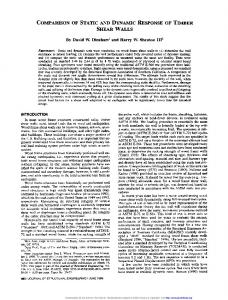
1.1. Stylise Facts about HCPI in Sierra Leone (Post-2017 Data) Headline Consumer Price Index (HCPI), a proxy for Inflation is very topical in Sierra Leone and more so, a primary objective of the central bank in maintaining stability to general prices of goods and services in the country (Jackson et al, forthcoming). As seen in Figure 1 below, the chart provide high frequency data for HCPI since 2007M01 to 2017M09; this is a representation of composite of all items in the basket which are weighted by the Central Statistical Office in Freetown. Prior to 2007, HCPI data were disaggregated for those in the capital city and the provincial towns. As seen, the highly time series data (normal and seasonally adjusted) shows upward / deterministic trend in inflation and this is as a result of the predominance of tradable influence of the CPI basket driven by the country’s reliance on the importation of basic commodity goods needed for consumption in the country. In order to keep track of the bank’s objective of monitoring price stability, staff in the research department would normally (quarterly) make use of econometric applications like EVIEWS to carry empirical study on simple methodology like the Box-Jenkins Autoregressive Moving Average and Autoregressive Integrated Moving Average [ARIMA] to forecast inflation dynamics which is fed into policy judgment for rates fixing in the country.
Figure 1: Graph Showing Plot of HCPI and HCPI_SA 2
ARIMA Forecast Comparison
220 200 180 160 140 120 100 80 07
08
09
10
11
12
HCP I
13
14
15
16
17
HCP I_S A
1.2. Hypothetical Question and Objective The main question that is set to be answered here is: Does STATIC forecast provide a better results than that of DYNAMIC forecast in ARIMA model? In this vein, the main objective here is to investigate the accuracy of the out-of-sample forecast for both Static and Dynamic approaches using HCPI variable. In addition to the aforementioned introduction, the rest of the paper is structure as follows: Section two present the Theoretical Framework and Methodology, which is also sub-divided into Time series models, Methodology, test description, and Data usage. Section three addresses the Empirical Results and discussion, while section four provide conclusion on the outcome and with some suggestions for policy makers in terms of a country’s peculiarity.
2. Theoretical Framework and Methodology
2.1. Time Series Model Literature Time series model is more common in using past movement of variable as a way of predicting future values / events. Unlike structural models which relates to the model at hand to forecast, time series models are not necessarily rooted on economic theory, while the reliability of the estimated equation is normally based on out-of-sample forecast performance as first observed by Stock and Watson (2003). Times series are mostly expressed by Autoregressive Moving Average (ARMA) models which was first produced by Slutsky (1927) and Wold (1938) as expressed in the following equation: 3
ARIMA Forecast Comparison
Yt = et – θ1et-1 – θ2et-2 – θ3et-3 - ………- θqet-q
[1]
Such a series is referred to as a moving average of order q, with the nomenclature MA(q); where Yt is the original series and et as error term in the series. As Yule (1926) suggested, the autoregressive process of the moving average series can be expressed as: Yt = ϕ1Yt-1 + ϕ2Yt-2 + ϕ3Yt-3 + …………. + ϕpYt-p +et
[2]
It is assumed that t, is independent of Yt−1, Yt−2, Yt−3, ... Yt−q . In this model, we are trying to fit the Box-Jenkins Autoregressive Integrated Moving Average (ARIMA) model, which is the generalised model of the non-stationary ARMA model represented by ARMA(p,q) and this can be written as: Yt = ϕ1Yt-1 + ϕ2Yt-2 + ϕ3Yt-3 + …+ ϕpYt-p +et – θ1et-1 - – θ2et-2…..- – θpet-p
[3]
Where, Yt is the original series, for every t, we assume that is independent of: Yt−1, Yt−2, Yt−3, …, Yt−p .
According to Hamjah (2014: 170-171), the following steps are worth considering when auctioning the Box and Jenkins approach to ARIMA forecasting: i. Preliminary analysis: Data at hand should conform to a stationary stochastic process. ii. Identification: specify the orders p, d, q of the ARIMA model so that it is clear the number of parameters to estimate and also recognition of the importance of autocorrelation functions in the model. iii. Estimate: efficient, consistent, sufficient estimate of the parameters of the ARIMA model (maximum likelihood estimator). iv. Diagnostics: Model to be checked for appropriateness using tests on the parameters and residuals of the model. Even when the model is rejected, still this is a very useful step to obtain information to improve the model. v. Usage of the model: Once tests outcomes are sufficiently passed or satisfies specification, it can then be used to interpret a phenomenon based on forecast outcome(s).
Other procedures worth using and more so, applied in this study include the following: -
Check normality assumption, proceed to the “Jarque-Bera” test, which measure goodness of fit from normality, based on the sample Kurtosis and skewness.
4
ARIMA Forecast Comparison
-
The “Ljung-Box” test can also be applied under the hypothesis that there is no autocorrelation in the residuals.
-
Autocorrelation Function [ACF] and Partial Autocorrelation Function [PAC] can also be used to detect the order of difference of Stationarity conditions.
-
Use of Akaike Information Criterion (AIC) and Bayesian Information Criterion (BIC) for model selection criterion.
2.2. Empirical Literature Chatfield (2001: 11), defined time series as an observed sequential data computed over a period of time; in many cases, such observation may be done for a single (univariate) or many (multi-variate) variables. For the purpose of this study, emphasis is paid to univariate time-series observation / analysis. In this vein, a univariate time-series refers to an observation that consists of single observations recorded sequentially through time, for example, the monthly unemployment rate (Klose, Pircher and Sharma, 2004).
In many cases, there is an underlying assumption when doing a time-series analysis, which is to do with the regularities expected of data as in the case with multivariate study. Klose et al (2004) carried sound univariate study as applied in the case with Austria; in this, they made use of Autointegrated Moving Average [ARIMA] model which proved to be a more robust means for forecast in comparison to a singular study on VAR model. They also provided some limitations, but on the whole, ARIMA was concluded to be a suitable choice of model.
Kelikume and Salami (2014) carried out independent investigation of inflation rate in Nigeria using VAR and ARIMA. They made use of CPI data obtained from the National Bureau of Statistics and the Central Bank Nigeria (CBN) during 2003 to 2012 to predict movements in the general price level. The study highlighted limitations in terms of its reliance on univariate analysis, but also brought to the fore some positive outcomes of using ARIMA model. It also outlined the limitation of using a single variable which may not necessarily have anything to compare with unless based on its past values. Bokhari and Feridun (2006) also carried out investigation using comparative univariate analysis of VAR and ARIMA to forecast inflation in Pakistan. In their analysis, ARIMA was seen to have 5
ARIMA Forecast Comparison
produced a better outcome in the forecast than that of a singular VAR study. Despite the fact that the study was able to unearth some issues around macroeconomic forecasting, it also brought to the fore the implication of such forecast technique for small scale macroeconomic model. The use of Univariate studies is also found to be very important and applicable in different areas of studies dealing with time series data; Taylor (2008) made use of this using ARIMA to forecast trends associated with intra-day arrivals by operators at a retail bank call centre in the UK. The study confirmed use of methods like "seasonal ARIMA modelling and AR modelling, an extension of Holt-Winters exponential smoothing for the case of two seasonal cycles, robust exponential smoothing based on exponentially weighted least absolute deviations regression and dynamic harmonic regression, a form of unobserved component state space modeling". The use of Univariate forecast is quite prominent given its quick response in finding solution to problems, as manifested in Taylor's (2003) research in forecasting short-term electricity demand using double exponential smoothening technique. Bianchi et al. (1998), in their Univariate study also made use of ARIMA modelling technique in determining seasonal forecasting daily arrivals at a telemarketing call center. In this study, supplemented their technique with intervention analysis as a way of controlling the presence of outliers, for which the resultant forecasts manifested an out-performance of the standard HoltWinters seasonal exponential smoothing. In as much as the positive side of using ARIMA model for forecasting univariate study is considered soundly echoed in modeling time series data, it was shown in Meyler, Kenny and Quinn (1998) study that ARIMA perform poorly compared to stand-alone VAR when applied to volatile and high frequency data. On a more positive note, Ho and Xie (1998) complemented ARIMA to be a more viable alternative model in terms of predicting performances.
2.3. Data Data used were extracted from the Statistics Sierra Leone database source for HCPI from 2007M1 to 2017M10. In order to smoothen out the series, data were seasonally using EVIEWS to remove issues of seasonality.
6
ARIMA Forecast Comparison
3. Empirical Results and Discussion The process commenced with a test of Stationarity for HCPI_SA using Phillips-Perron at 1st level as shown in Table 1; with the application of absolute value concept, the result indicate that ARIMA is the appropriate methodology to be applied as opposed to ARMA. 3.1. Table1: Unit Root Result for Headline Consumer Price Index D(HCPI_SA)
Phillips-Perron test statistic Test critical values:
Adj. t-Stat
Prob.*
-5.580481
0.0000
1% level
-4.031899
5% level
-3.445590
10% level
-3.147710
This is an indication of the method to be proceeded by determining the order of the AR and MA processes and the suitability of best model that will bring about the best forecast outcome given the nature of data used. At first level, the variable is highly significant with its probability value equal to 0.
3.2.Selection and Iteration for Best Model Estimation Using the automated ARIMA forecast process, EVIEWS have made the best model selection of (6,0)(0,0) as shown in Figure 2.
Figure 2: Automatic ARIMA Model Estimation Choice
7
ARIMA Forecast Comparison
This is based on the use of a single variable, which is HCPI and for which the lag of it is used to determine future occurrences. The estimation output below (4,1,0) in Table 2 is considered the best after series of iterations, with the lowest AIC value and an Inverted AR Root value