Comparison of Implementations of Gaussian Mixture. PHD Filters. Michele Pace, Pierre Del Moral and François Caron. INRIA Bordeaux Sud Ouest. Institut de ...
Comparison of Implementations of Gaussian Mixture PHD Filters Michele Pace, Pierre Del Moral and Fran¸ cois Caron INRIA Bordeaux Sud Ouest Institut de Math´ematiques de Bordeaux Bordeaux, France {Michele.Pace; Pierre.Del-Moral; Francois.Caron}@inria.fr Abstract – The Probability Hypothesis Filter, which propagates the first moment, or intensity function, of a point process has become more and more popular to address multi-tracking problems. Under linear-Gaussian assumptions, the intensity function takes the form of a mixture of Gaussian kernels. As the number of elements increases exponentially over time, deterministic pruning and merging steps are commonly used to keep the complexity bounded. In this paper, we study alternative stochastic strategies. The different strategies are compared on different scenarios. A new pruning strategy that maintains confirmed targets is also proposed.
techniques are generally used to keep the complexity bounded. Such deterministic procedures, however, lead to biased estimates of the weights, and we study here an alternative stochastic procedure. This procedure can be seen as a stochastic version of both N-best and thresholding deterministic procedures. We also propose in Section 5 a multitarget-tracker adapted pruning that maintains over time a list of confirmed targets to avoid the pruning of existing targets when undetected.
2
GMPHD Filter
2.1 Keywords: Multi-Target Tracking, Resampling, Probability Hypothesis Filter, Gaussian Mixture.
1
Introduction
Multi-target tracking aims at estimating the states of a possibly unknown number of targets in a given surveillance region. The available sensors generally collect several measurements which may correspond to some clutter or to the targets of interest, if detected. The sensors typically lack the ability to associate each measurement to its originating target or to the clutter. Hence, one has to solve simultaneously three problems: data association, the estimation the number of targets if this number is unknown and estimate their states. Numerous algorithms have been proposed in the literature to address such problems [1]. Among these algorithms, the Probability Hypothesis Filter [7, 8] has gained a lot of popularity over the past years. The filter propagates the first moment of a point process and thus gives an alternative and elegant solution to the data association problem. When the single target dynamics and measurement models are linear and Gaussian, or can be approximated by linear-Gaussian models, the Gaussian Mixture PHD filter [13] (GMPHD) represents the first moment of the point process by a Gaussian mixture. As the number of elements increases over time, pruning and merging
Notations
The set of targets tracked at time t is modeled as a point process [7, 14, 8]. We note Xt = {Xt,1 , . . . , Xt,Kt } ∈ F(X ) the set of targets at time t, where F(X ) is the set of finite subsets of X . Let ( ) Xt = ∪x∈Xt−1 St|t−1 (x) ∪ (∪x∈Xt−1 Dt|t−1 (x)) ∪ Nt (1) where • St|t−1 (x) is the random set of targets that survived at time t from targets x ∈ Xt−1 , • Dt|t−1 (x) is the random set of target that spawn from x ∈ Xt−1 and • Nt is the random set of targets born at time t.
To simplify the exposition, we will assume in the following that there is no spawning, hence Dt|t−1 (x) = {∅}. Let Yt = {Y1 , . . . , YNt } the set of measurements at time t and Yt = Γt ∪ (∪x∈Xt Gt (x))
(2)
where Gt (x) is the random set of measurements coming from target x ∈ Xt and Γt is the set of measurements coming from clutter at time t.
A random set X ∈ F(X ) can be equivalently represented by a counting measure NX on the space of borelians of X, defined by ∑ NX (S) = 1S (x) = |X ∩ S| (3) x∈X
where 1S (x) = 1 if x ∈ S, 0 otherwise, and |A| is the number of elements in the set A. Using this representation, the first moment, or intensity measure, of X ∈ F(X ) is defined by V (S) = E [N (S)]
(4)
The intensity V (S) in a region S provides the mean number of elements X in S. The density ν : X → [0, +∞[ of the intensity measure V w.r.t. the Lebesgue measure is called the intensity function. It is also known in the tracking community as the ∫ “Probability Hypothesis Density” or PHD. We have S ν(x)dx = E [N (S)] = E [|X ∩ S|]. The maxima of ν correspond to points in X with high local concentration of targets. The intensity function can therefore be used to estimate X. This post-processing, which is crucial in PHD-based algorithms, will be left aside in this paper, and we will focus on the faithful approximation of the intensity function ν.
2.2
PHD filter
The PHD filter propagates the first moment of the posterior distribution of the point process Xt . Let νt|t and νt|t−1 be respectively the intensity functions associated to the posterior point processes Xt |Y1:t = y1:t and Xt |Y1:t−1 = y1:t−1 . We have the following recursions [7] ∫ νt|t−1 (x) = pS,t ft|t−1 (x|u)νt−1|t−1 (u)du+γt (x) (5) X
where ft|t−1 (x|u) is the evolution density of a single target at time t, pS,t is the survival probability of a target and γt (x) is the birth intensity function of new targets at time t and
2.3
PHD recursions Gaussian case
the
linear-
The recursions (5) and (6) imply the computation of integrals that cannot generally be calculated analytically. Under some linear-Gaussian assumptions, detailed later in this paragraph, posterior intensity functions take the form of a mixture of Gaussian densities [13]. We assume that ft|t−1 (xt |xt−1 ) = N (xt ; Ft xt−1 , Qt ) gt (yt |xt ) = N (yt ; Ht xt , Rt ) where N (x; µ, Σ) is the Gaussian pdf of mean µ and covariance matrix Σ evaluated in x. Ft , Ht , Qt and Rt are respectively known evolution, observation and noise covariance matrices. We further assume that pS,t (x) = pS,t pD,t (x) = pD,t and that the birth intensity takes the form of a mixture of Gaussian ∑
mγ,t
γt (x) =
πγ,t,k N (x; µγ,t,k , Σγ,t,k )
k=1
where mγ,t , πγ,t,k , µγ,t,k et Σγ,t,k are fixed parameters. Assume at time t − 1 the posterior intensity takes the form of mixture of Gaussians ∑
mt−1
νt−1|t−1 (x) =
πt−1,k N (x; µt−1,k , Σt−1,k )
k=1
We have therefore the following prediction and update steps: • Prediction ∑
mt−1
νt|t−1 (x) = pS,t
πt−1,k N (x; µS,t|t−1,k , ΣS,t|t−1,k )
k=1
∑
mγ,t
+
νt|t (x) = (1 − pD,t (x))νt|t−1 (x) ∑ pD,t (x)ht (y|x)νt|t−1 (x) ∫ + (6) κt (y) + X pD,t (u)ht (y|u)νt|t−1 (u)du y∈Y
πγ,t,k N (x; µγ,t,k , Σγ,t,k )
k=1 mt|t−1
:=
∑
πt|t−1,k N (x; µt|t−1,k , Σt|t−1,k )
k=1
t
where ht (y|x) is the single target likelihood, pD,t (x) is the probability of detection and κt is the clutter intensity at time t. These recursions are based on the hypothesis that the processes Xt|t et Xt|t−1 can be well approximated by Poisson processes. This simplification allows an analytical expression for the posterior intensity function recursions, but implicitly makes the assumption that the higher order moments are negligible [8]. Proofs of these recursions can be found in [7, 12].
in
(7) where the pairs (µS,t|t−1,k , ΣS,t|t−1,k ) are calculated from (µt−1,k , Σt−1,k ) using a Kalman filter prediction step. • Estimation νt|t (x) = (1 − pD,t )νt|t−1 (x) +
t|t−1 ∑ m∑
y∈Yt
k=1
πt,k (y)N (x; µt,k (y), Σt,k (y))(8)
where the weights are given by πt,k (y) =
Gaussian to survive the following steps. Basically, the algorithm automatically sets a threshold value of 1/c; all the weights above this threshold are kept, while the others are resampled. The resampling scheme is described in Algorithm 1.
pD,t πt|t−1,k qt,k (y) ∑mt|t−1 κt (y) + pD,t l=1 πt|t−1,l qt,l (y)
qt,l (y) = N (y; ybt|t−1,l , St|t−1,l ) and the pairs (µt,k (y), Σt,k (y)) et (b yt|t−1,l , St|t−1,l ) using a Kalman Filter update step.
3
Algorithm 1 Fearnhead-Clifford resampling algorithm ⋆ • Let πt,k be the N normalized weights at time t. Calculate the unique solution c of N = ∑M ⋆ min(π , 1) t,k k=1
Sampling-Resampling strategies for GM-PHD filters
⋆ • For k = 1, . . . , M , if πt,k > 1/c then place it in set 1; otherwise place it in set 2. Assume there are L elements in set 1.
The total number mt of elements in the Gaussian mixture follows the recursion: mt = (mt−1 + mγ,t )(1 + |Yt |)
where |Yt | denotes the number of measurements at time t. Although the number of elements increases at a lesser rate than in the classical data association problem, it is nonetheless necessary to make approximations, and we will assume in the following that we want to keep the overall number of elements at time t equal to a fixed number N . General methods use deterministic pruning and merging. We propose in this section to study the use of an unbiased resampling strategy as proposed in [5]. Assume that we have M Gaussian terms with weights πt,k and we want to obtain M Gaussian terms with weights π et,k such that only N among them have nonzero weights.
3.1
Deterministic resampling for GMPHD
The main approach consists in using two steps of pruning and merging to keep the number of Gaussian terms bounded. Gaussians whose Mahalanobis distance is less than a given threshold U are fused, and the N Gaussians with highest weights among them are kept. Assume that we rank the weights, then we have { π et,k = πt,k If rank(πt,k ) ≤ N π et,k = 0 Otherwise The error made by using this strategy has been studied in [3]. Clearly, this pruning strategy is biased as E[e πt,k ] ̸= πt,k for lower weights. We propose in the following section to use an unbiased resampling scheme that leaves a chance for lowest weights to be selected.
3.2
• Use the stratified sampling of Carpenter et al. [2] to resample N − L Gaussians from set 2. The expected number of times that each particle is resampled is proportional to its weight.
(9)
• The new set of Gaussians consists of the L elements in set 1, each given its original weight, and the N − L elements in set 2, each assigned a weight 1/c.
The average running time of the algorithm is O(N ). The resampling scheme has the following properties [5] (a) E[e πt,k ] = πt,k (unbiasedness) (b) The support of π et has no more than N points [∑ ] M 2 (c) E (e π − π ) is minimized k,t k=1 t,k
4 4.1
Experiments Models
For illustration purposes, consider a monodimensional scenario with an unknown and time varying number of targets observed in clutter over the surveillance region [-100,100]. The state of each target xt = [pt , p˙t ] consists of position and velocity, while the measurement is a noisy observation of the position component. Each target has a survival probability pS,t = 0.995, a probability of detection pD,t = 0.95 and follows a linear Gaussian dynamics. The process model is as follows: [ ] [ ] 1 T 0 xt+1 = xt + ut (10) 0 1 T with ut ∼ N (0, σu2 ) and σu = 0.7. Each target, if detected, generates an observation according to:
Optimal resampling GM-PHD
We propose here to use the stochastic resampling algorithm proposed by Fearnhead and Clifford [5]. This procedure is quite similar to the N -best and thresholding strategies, but it will leave a chance to some low-weight
yt =
[
1 0
]
xt + vt
(11)
The sampling period T = 1 and vt ∼ N (0, σv2 ) with σv = 1. The birth intensity is defined as γb = 0.35N (.; xb , Qb ) where xb = [0, 0]T and
[ Qb =
20 0 0 1
]
reports the errors for the first 6 time steps using the complete intensity as reference function.
The clutter is Poisson with intensity λc . If a target exits from the surveillance region it is eliminated from the simulation. Each simulation lasts 100 time steps and to avoid short-living targets the latest birth-time is set to the 30th time step. While the structure of this model is simple, the clutter intensity and the number of miss detections make the filtering of the scenarios non trivial. Figure 1 shows a realization of a scenario.
Time step T=1 T=2 T=3 T=4 T=5 T=6
Time
T=1 T=2 T=3 T=4 T=5 T=6 T=7 T=8 T=9 T=10
x
50
0
−50
0
10
20
30
40
50
60
70
80
90
Figure 1: True target positions (green) and clutter (black).
In order to assess the effect of different resampling strategies we consider the L2 norm of the error function between the posterior PHD intensity νt|t provided by the GMPHD filter, and a reference function νref : |νt|t − νref |2 dµ
E(νt|t ,νref ) =
8 20 79 171 311 612 1227 2333 5622 8327
I.
PT 10−10
I.
0.07498 0.45724 1.0614 1.5245 1.4247 1.8215 2.5848 2.9292 2.9972 2.1249
mer. 5 4 5 14 19 19 26 28 25 35 36
0.07498 0.45697 1.3956 1.5632 1.3206 1.793 2.3956 2.9556 3.031 2.1434
Table 2: Number of Gaussian terms (column 2 and 4) and integral of the posterior PHD with pruning and merging.
Reference function
(∫
PT 10−10
100
time step
4.2
I. 0.07498 0.45724 1.0614 1.5245 1.4247 1.8215
Table 1: Number of terms in the first GMPHD posteriors using a test scenario with 2 targets and λc = 5. No pruning or merging are used.
100
−100
N.Gaussian Terms 8 36 407 2448 12245 73476
) 21 (12)
S
The integral is computed numerically on a bidimensional grid where S covers a sufficiently large subset of the domain. One natural choice for the reference function would be the posterior intensity obtained without pruning and merging, but the computational burden of this approach leads to the necessity of finding good substitutes. In order to compare possible reference functions, it is possible to consider the complete posterior on a limited number of time steps. Table 1 reports the number of Gaussian terms and the mass of the PHD intensity on a test scenario with two targets and clutter intensity λc = 5 when no merging and no pruning is used. Despite their rapid explosion, most of the terms give no contribution at all, as their weights fall under machine precision rapidly. The elimination of these terms by using a small pruning threshold (for example 10−10 as in Table 2), determines a sharp reduction in the number of modes and an error under machine precision. When merging is used, their number decreases even more, but errors begin to be noticeable. Table 3
Time
err PT 10−10
err. PT 10−10 , MT=5
T=1 T=2 T=3 T=4 T=5 T=6
1.1065e-038 2.456e-034 7.9324e-021 1.3978e-019 4.652e-019 5.311e-018
2.2738e-008 0.001125 0.0062382 0.02316 0.04974 0.060487
Table 3: Errors w.r.t the reference function of Table 1. The computational cost of building reference functions using only pruning is still too high on long scenarios, especially for Monte Carlo validations. Results using different merging thresholds suggest that a good compromise between the computational load and the error is obtained by using a pruning threshold P T = 10−10 and a merging threshold M T = 1.
4.3
Results
The following resampling methods are evaluated: • N-Best: After the GMPHD update, the N terms with greater weight are kept. All the other terms are eliminated. The resulting Gaussian mixture is used as input for the next step. • Threshold : After the GMPHD update, all the terms whose weight is above a pre-defined threshold are kept. • Fearnhead-Clifford resampling: The Fearnhead-Clifford resampling is used to resample M terms from the updated mixture. M =
{5, 10, 20}. If the mixture has less than M terms, all of them are kept. Num terms in posterior PHD.
Reference NBEST−5 NBEST−10 P.TRESHOLD−01 P.TRESHOLD−001 FC−5 FC−10 FC−20
100
80
60
40
20 10 5 0
0
10
20
30
40
50
60
70
80
90
100
Time step
Figure 2: Number of Gaussian terms in the posterior PHD with different resamplig strategies (100 iterations, birth intensity 0.35)
Error w.r.t reference function
0.25 NBEST−5 NBEST−10 P.TRESHOLD−01 P.TRESHOLD−001 FC−5 FC−10 FC−20
0.2
0.15
0.1
0.05
0
0
10
20
30
40
50
60
70
80
90
100
Time step
Figure 3: Error in the posterior PHD with different resamplig strategies w.r.t the reference function. (100 iterations, birth intensity 0.35) 0.14
Error w.r.t reference function
The results are obtained by processing randomlygenerated scenarii with a number of targets N ∈ [2 . . . 5], and clutter intensity parameter λc ∈ [2 . . . 5]. The target dynamics and the birth intensity have the same parameters as described in section 4.1. The reference function is computed for each scenario using pruning threshold P T = 10−10 and merging threshold M T = 1. The average number of terms in the PHD approximation and the average error for the different resampling methods are reported in Figures 2 and 3. When the same parameter is used, the deterministic methods always outperforms the stochastic resampling in terms of computational cost and quality of the results. Using a pruning threshold generally provides better results, but the threshold has to be chosen carefully, by considering the clutter level and the miss-detection probability. The performance of the Threshold strategy is also influenced by the level of the birth intensity (Figure 4 and 7). Similar conclusions has been reported in [13] and [9] where it is observed that selecting the highest peaks (corresponding to the N-Best resampling) may generate unreliable state estimates due to terms with very small weights. As we measure the error w.r.t a reference function the better result obtained by setting a threshold is due to the contribution of all the additional terms that are sufficiently significant to be above the pruning threshold but not enough to be selected by the N-Best. Figures 2 and 3 report the average number of terms which are selected by the different methods and the average errors on a Monte Carlo simulation. The Fearnhead-Clifford resampling and the NBest maintain the computational cost bounded as they produce a posterior PHD with a fixed number of terms. As the targets may disappear with probability 1 − pS,t and are eliminated when they exit from the surveillance zone, their number tends to decrease over time, and so does the average error. The stratified resampling used in the Fearnhead-Clifford algorithm degrades the performance in a way that the error introduced by using a parameter N is comparable with the error of N-Best with parameter N/2.
120
NBEST−5 NBEST−10 P.TRESHOLD−01 P.TRESHOLD−001 CF−5 CF−10 CF−20
0.12
0.1
0.08
0.06
0.04
0.02
0
0
10
20
30
40
50
60
70
80
90
100
Time step
One disappointing result is indeed the poor performance of the Fearnhead-Clifford resampling compared to the simpler deterministic methods. The unbiasedeness of the choice of the Gaussian terms at a greater computational cost does not provide any advantage in terms of the approximation error. Fig. 5 plots the weights of the updated Gaussian terms at different time steps and the Fearnhead-Clifford threshold. Once again, after the update step most of the terms have very low weights, which cause a waste of computational time if not correctly pruned.
Figure 4: Error in the posterior PHD using different resamplig strategies w.r.t the reference function. (100 iterations, birth intensity 0.15)
4.4
Resampling efficiency
As the error is an inverse measure of the quality of the posterior and the cost is proportional to the number terms it has, we measure the resampling efficiency with η = 1/(et Nt ), where et is the error w.r.t the reference
0.2 3
10
0.15
NBEST−5 NBEST−10 P.TRESHOLD−01 P.TRESHOLD−001 FC−5 FC−10 CF−20
0.1 0.05 0
2
10
0
10
20
30
40
50
60
70
80 Efficiency.
0.2 0.15 0.1
1
10
0.05 0
0
10
20
30
40
50
60
70
80
90
0.4 0
10
0.3
0
10
20
30
40
50 Time step
60
70
80
90
100
0.2 0.1 0
0
10
20
30
40
50
60
70
80
90
Figure 5: Fearnhead-Clifford threshold and weights of the terms in the posterior Gaussian mixture at different time steps. function and Nt the number of Gaussian terms in the posterior PHD approximation. If a method produces no terms in the posterior Nt = 0 the efficiency is not computed. Figure 6 reports the efficiencies in a logarithmic scale for the methods discussed. The deterministic acceptance of all the terms above a threshold provides the best cost-quality ratio. The Fearnhead-Clifford resampling has, on the contrary, a poor performance. 3
10
NBEST−5 NBEST−10 P.TRESHOLD−01 P.TRESHOLD−001 FC−5 FC−10 FC−20
2
Efficiency
10
1
10
0
10
−1
10
0
10
20
30
40
50
60
70
80
90
100
Time step
Figure 6: Efficiency of different resamplig strategies w.r.t the reference function. (100 iterations, birth intensity 0.35)
Figure 7: Efficiency of different resamplig strategies w.r.t the reference function. (100 iterations, birth intensity 0.15) sian terms that have generated the estimates. In order to perform the peak-to-track association as a post processing operation the GMPHD recursion is modified to maintain and propagate the labels associated to the Gaussian terms. The information about confirmed tracks can be exploited during the GMPHD resampling to alleviate the loss of targets in case of miss detections. The rapid fall of the weights below the pruning threshold may cause the elimination of an active target and a delay of several time steps before its reactivation. These errors can be avoided by preventing the Gaussian terms to be pruned if they correspond to confirmed tracks until they reach a more conservative deactivation threshold. In order to evaluate this target-tracker-adapted pruning criterion we consider the Optimal Subpattern Assignment (OSPA) Metric with cutoff parameter c = 20. As it penalizes both the relative differences in cardinality estimate as well as the distance of true targets from their estimates, it is generally considered a good and consistent measure of the quality of a filter output. Moreover it is independent from the geometry of the scenario and well defined in case of zero-cardinality Random Finite sets. Details on this metric can be found in [11]. We focus especially on the cardinality error component of the OSPA, defined as: (c)
e¯p,card (X, Y ) := (c)
5
Multitarget-tracker pruning
adapted
As the GMPHD filter does not provide identities of individual state estimates, techniques to construct the tracks from the posterior mixture are required. These techniques as well as different implementations of multitarget trackers have been investigated in [6], [10], [4]. Multi-target trackers maintain at each time step a list of confirmed targets as well as the labels of the Gaus-
( cp (n − m) ) p1 n (c)
if m ≤ n, and e¯p,card (X, Y ) := e¯p,card (Y, X) if m > n. X = {x1 , . . . , xm } and Y = {y1 , . . . , yn } are the subsets of ground-truth positions and target estimates and p = 2 the order of the metric. Figure 9 reports the average OPSA distance and the average cardinality error in a Monte Carlo evaluation of 500 scenarios. The target detection probability has been lowered to pD,t = 0.9, the probability of target survival pS,t = 0.995 and the birth intensity is a Gaussian mixture composed by three terms centered respectively in [−50, 0]T , [0, 0]T and [50, 0]T with σp = 20 and σv = 1. The weights
of birth intensity’s terms are lowered to 0.15 to make it more difficult for the GMPHD filter to catch new targets or to recover from miss-detections. Each simulation contains a random number of targets N ∈ [2 . . . 5], and a Poisson number of false observations with mean λc ∈ [2 . . . 5] uniformly distributed over the surveillance zone. Pruning threshold is set to 0.1; targets are extracted from the posterior Gaussian mixture if their weights are above 0.5. By using the information about the active targets which is provided by the multi-target tracker, it is possible to avoid the pruning of Gaussian terms corresponding to confirmed tracks until their weights reach the elimination threshold (10−3 in the simulation).
Figure 8: Schematic representation of the target confirmation and elimination events triggered by the growth of the Gaussian weight. An elimination threshold is added in order to avoid the pruning of confirmed terms until they reach a more conservative level.
keep the algorithm computationally feasible. We have evaluated the stochastic resampling method proposed by Fearnhead and Clifford which provides an automatically chosen threshold and guarantees the uniqueness and unbiasedness of the resampled elements. Moreover, it leaves a probability to low-weighted Gaussian terms to survive. Unfortunately, Monte Carlo validations on different scenarios and with different parameters have demonstrated that deterministic strategies always outperform the Fearnhead-Clifford resampling in approximating the posterior PHD Gaussian mixture. One issue with current deterministic algorithms is that when a target goes undetected the mass of the corresponding term decreases rapidly and once deleted it may take several time steps to be reactivated, especially if the clutter process is intense and the detection probability relatively low. We proposed to tackle the problem using the multi-target tracker algorithm. The information on confirmed tracks can be effectively exploited in the pruning step to postpone the elimination of Gaussian terms until their weights reach a value corresponding to the almost sure target disappearance. Monte Carlo validations by using the OSPA metric confirmed the improvement of the filtering results when this strategy is adopted. Acknowledgments The authors would like to thank Dann Laneuville and J´er´emie Houssineau from DCNS-SIS for the fruitful discussions which provided us with more insights on the application of PHD filters to real naval scenarios.
References OSPA distance
20 Without MT−Tracker With MT−Tracker 15
10
5
OSPA Cardinality Error
0
0
10
20
30
40
50
60
70
80
90
100
15 Without MT−Tracker With MT−Tracker
[2] J. Carpenter and P. Clifford and P. Fearnhead, “Improved particle filter for nonlinear problems” IEE Proceedings Radar Sonar and Navigation, 1999, Vol. 146, pp. 2–7.
10
5
0
0
10
20
30
40
50
60
70
80
90
100
Time steps
Figure 9: OSPA error and cardinality error in 500 simulated scenarios using a target-tracker-adapted pruning criterion.
6
[1] Y. Bar-Shalom and X. Rong Li, “Multitargetmultisensor tracking: principles and techniques” YBS Publishing, 1995.
Conclusions
In this paper we analyzed deterministic and stochastic pruning strategies for the GMPHD filter in order to
[3] D. Clark and B.N. Vo, “Convergence analysis of the Gaussian mixture PHD filter” IEEE Transactions on Signal Processing, 2007, Vol. 55, pp. 1204– 1212. [4] D. Clark and J. Bell, “Data Association for the PHD Filter” International Conference on Intelligent Sensors, Sensor Networks and Information Processing, 2005, Vol. 55, pp. 217–222. [5] P. Fearnhead and P. Clifford, “Online Inference for Hidden Markov models” Journal of the Royal Statistical Society Series B, 2003, Vol. 65, pp. 887– 899.
[6] K. Panta and D. Clark and B.N. Vo, “An Efficient Track Management Scheme for the GaussianMixture Probability Hypothesis Density Tracker” Intelligent Sensing and Information Processing, 2006, pp. 230–235. [7] R. Mahler, “Multi-Target Bayes filtering via firstorder multi-target moments” IEEE Transactions on Aerospace and Electronic Systems, 2003, Vol. 39, pp. 1152–1178. [8] R. Mahler, “PHD filters of higher order in target number” IEEE Transactions on Aerospace and Electronic Systems, 2007, Vol. 43, pp. 1523–1543. [9] K. Panta, “Multi-Target Tracking Using 1st Moment of Random Finite Sets” Ph.D. dissertation, Department of Electrical and Electronic Engineering, University of Melbourne, 2007. [10] N. Pham and W. Huang and S. Ong, “Maintaining track continuity in GMPHD filter” International Conference on Information, Communications and Signal Processing, 2007. [11] D. Schuhmacher and B.T. Vo and B.N. Vo, “A Consistent Metric for Performance Evaluation of Multi-Object Filters” IEEE Transactions on Signal Processing, 2008, Vol. 56, pp. 3447–3457. [12] S.S. Singh and B.N. Vo and A. Baddeley and S. Zuyev, “Filters for spatial point processes” SIAM Journal of Control Optimization, 2009, Vol. 48, pp. 2275–2295. [13] B. Vo and W. K. Ma, “The Gaussian mixture Probability Hypothesis Density Filter” IEEE Transactions on Signal Processing, 2006, Vol. 54, pp. 4091–4104. [14] B. Vo and S. Singh and A. Doucet, “Sequential Monte Carlo methods for Bayesian Multi-target filtering with Random Finite Sets” IEEE Transactions on Aerospace and Electronic Systems, 2005, Vol. 41, pp. 1224–1245.