will define the different kinds of matrices of a graph, namely the adjacency matrix, the Laplacian ... The greatest integer r such that G contains an independent set of size .... of some term, i.e. they are the maximum, minimum of some function: 10 ...
Diploma Thesis:
Comparison of Spectral Methods Through the Adjacency Matrix and the Laplacian of a Graph
Philipp Zumstein
submitted 28. February 2005 at ETH Z¨ urich
Prof. Dr. Emo Welzl
Dr. Tibor Szab´o
2
Contents 0 Preface
5
1 Preliminaries 1.1 Graph Theory . . . . . . . . . . . . . 1.2 Matrix Theory . . . . . . . . . . . . 1.2.1 Basics about Eigenvalues . . . 1.2.2 Symmetric Matrices . . . . . 1.2.3 Positive Semidefinite Matrices 1.3 Asymptotic notations . . . . . . . . .
. . . . . .
. . . . . .
. . . . . .
. . . . . .
2 Spectral graph theory 2.1 Definitions and Basic Facts . . . . . . . . . . 2.1.1 The Adjacency Matrix . . . . . . . . 2.1.2 The Laplacian . . . . . . . . . . . . . 2.1.3 The normalized Laplacian . . . . . . 2.1.4 Relations between the Adjacency and 2.2 The theory of nonnegative matrices . . . . . 2.3 Trace of a Matrix . . . . . . . . . . . . . . . 2.4 Eigenvectors . . . . . . . . . . . . . . . . . . 2.5 Rayleigh quotient . . . . . . . . . . . . . . . 2.6 Interlacing . . . . . . . . . . . . . . . . . . . 2.6.1 Interlacing Theorems . . . . . . . . . 2.6.2 Interlacing for Independent Set . . . 2.6.3 Interlacing for Hamiltonicity . . . . . 2.7 Gerschgorin’s Theorem . . . . . . . . . . . . 2.8 Majorization . . . . . . . . . . . . . . . . . . 2.9 Miscellaneous . . . . . . . . . . . . . . . . .
. . . . . .
. . . . . .
. . . . . .
. . . . . .
. . . . . .
. . . . . .
. . . . . .
. . . . . .
. . . . . . . . . . . . . . . . . . . . . . . . . . . . . . . . the Laplacian . . . . . . . . . . . . . . . . . . . . . . . . . . . . . . . . . . . . . . . . . . . . . . . . . . . . . . . . . . . . . . . . . . . . . . . . . . . . . . . . . . . . . . . .
. . . . . . . . . . . . . . . . . . . . . .
. . . . . .
7 7 9 9 10 11 12
. . . . . . . . . . . . . . . .
13 13 13 16 19 21 23 27 32 36 39 39 41 42 42 44 45
3 Cauchy-Schwarz and other Inequalities 47 3.1 Cauchy-Schwarz Inequalitiy . . . . . . . . . . . . . . . . . . . 47 3.2 An inequality . . . . . . . . . . . . . . . . . . . . . . . . . . . 48 3
3.3
Some Spectral Technique . . . . . . . . . . . . . . . . . . . . . 50
4 Pseudo-random graphs 4.1 Models . . . . . . . . . . . . . . . . . 4.2 Basics about Pseudo-random graphs 4.3 Edge Connectivity . . . . . . . . . . 4.4 Maximum Cut . . . . . . . . . . . . . 4.5 Vertex Connectivity . . . . . . . . . . 4.6 Independent Set . . . . . . . . . . . . 4.7 Colorability . . . . . . . . . . . . . . 4.8 Hamiltonicity . . . . . . . . . . . . . 4.9 Small subgraphs . . . . . . . . . . . .
. . . . . . . . .
. . . . . . . . .
. . . . . . . . .
. . . . . . . . .
. . . . . . . . .
. . . . . . . . .
. . . . . . . . .
. . . . . . . . .
. . . . . . . . .
. . . . . . . . .
. . . . . . . . .
. . . . . . . . .
. . . . . . . . .
. . . . . . . . .
55 55 56 63 66 68 70 72 73 73
5 Tur´ an’s Theorem 5.1 Classical Tur´an’s Theorem . . . . 5.2 Generalization to (n, d, λ)-graphs 5.3 Comments about Chung’s paper . 5.3.1 Lemmas . . . . . . . . . . 5.3.2 Negligence of the λ2 -term
. . . . .
. . . . .
. . . . .
. . . . .
. . . . .
. . . . .
. . . . .
. . . . .
. . . . .
. . . . .
. . . . .
. . . . .
. . . . .
. . . . .
83 83 85 86 87 89
. . . . .
. . . . .
Appendix 91 List of Definitions . . . . . . . . . . . . . . . . . . . . . . . . . . . . 91 List of Theorems . . . . . . . . . . . . . . . . . . . . . . . . . . . . 92 Maple-Code . . . . . . . . . . . . . . . . . . . . . . . . . . . . . . . 93 Bibliography
96
4
Chapter 0 Preface Graph theory and linear algebra are two beautiful fields of mathematics and spectral graph theory lies in their intersection. More exactly, spectral graph theory deals with the properties of a graph in relationship to the eigenvalues and eigenvectors of some associated matrix. First, in chapter 1 we will collect the preliminaries of graph and matrix theory and introduce the usual asymptotic notations. Then in chapter 2 we will define the different kinds of matrices of a graph, namely the adjacency matrix, the Laplacian and the normalized Laplacian. After some basic facts we will describe different methods that exist in spectral graph theory and give some applications. In chapter 3 we will state the Cauchy-Schwarz and other inequalities. We will also discover spectral techniques using the Cauchy-Schwarz Inequality. After that we are ready to discuss pseudo-random graphs. Pseudo-random graphs are graphs which behave like random graphs. In chapter 4 we will define the concept of pseudo-random graphs via eigenvalues. There are two approaches to do that. One considers the spectrum of the adjacency matrix and the other the spectrum of the normalized Laplacian. The first approach is mostly easier to apply but only adaptable for d-regular graphs. We will then generalize some statements of the survey paper about pseudo-random graphs by Krivelevitch and Sudakov [18] for the normalized Laplacian. Finally, in chapter 5 we will discuss Tur´an’s Theorem and some attempts to extend this theorem for pseudo-random graphs.
5
Acknowledgement. I would like to thank my advisor Dr. Tibor Szab´o and Prof. Emo Welzl. Also, I would like to thank everyone who read parts of this thesis and made suggestions to its improvement.
6
Chapter 1 Preliminaries 1.1
Graph Theory
Most of the material of graph theory is taken from West [30] and Jukna [15]. A (simple) graph is a pair G = (V, E) consisting of a set V , whose elements are called vertices, and a family E of 2-element subsets of V , whose members are called edges. A directed graph is pair G = (V, E) consisting of a set V (vertices) and a set E (edges) of ordered pairs of V . The first vertex of the ordered pair is the tail of the edge and the second is the head ; together they are called endpoints. In the following the concept of directed graph is rarely needed. We continue now the discussion about (simple) graphs. A subgraph of G = (V, E) is a pair H = (W, F ) such that W ⊆ V, F ⊆ E. An induced subgraph of G = (V, E) is a set of vertices W and all edges from G which have both endpoints in W ; the induced subgraph of G spanned by the vertices is denoted by G[W ]. A vertex v is incident with an edge e if v ∈ e. Two vertices u, v of G are adjacent, or neighbors, if {u, v} is an edge of G. We denote the set of all neighbors of u by N (u). We will write u ∼ v if u and v are adjacent. A vertex which has no neighbors is called isolated. The number du of neighbors of a vertex u is its degree. A graph is called d-regular if all degrees are d. The maximum degree of a graph G is denoted by ∆(G) (or simply ∆) and the minimum degree by δ(G) (or simply δ).
7
Lemma 1.1 Let G = (V, E) be a graph. Then X dv = 2|E|. v∈V
A walk of length k in G is a sequence v0 , e1 , v1 , ..., ek , vk of vertices and edges such that ei = {vi−1 , vi } for all i. A walk without repeated vertices is a path. A cycle is a closed path, i.e. a path with an edge from the first vertex to the last one. A component in a graph is a maximal set of vertices such that there is a path between any two of them. A graph is connected if it consists of one component. Mutatis mutandis: A directed graph is strongly connected if there exists a directed path between any two of the vertices. A Hamiltonian cycle of a graph G = (V, E) is cycle of length n = |V |, i.e. the cycle goes through all vertices once. A graph is called Hamiltonian if it consists a Hamiltonian cycle. An independent set in a graph is a set of vertices with no edges between them. The greatest integer r such that G contains an independent set of size r is the independence number of G, and is denoted by α(G). A complete graph or clique is a graph in which every pair of vertices is adjacent. The complete graph on n vertices is denoted by Kn . A graph is bipartite if its vertex set can be partitioned into two independent sets. The complete bipartite graph is denoted by Kn,m where n is the size of one part and m is the size of the other part. The star Sn = K1,n−1 is the complete bipartite graph on n vertices in which one part has size 1. More generally, a graph is r-partite if its vertex set can be partitioned into r independent sets. Lemma 1.2 G is bipartite ⇐⇒ G contains no odd cycle. Let G be a graph and S a subset of vertices. G − S is the graph obtained from G by deleting the vertices S (and all edges incident to some vertex from S). The connectivity of G, written κ(G), is the minimum size of a vertex set S such that G − S is disconnected. The connectivity of the complete graph Kn is defined as n−1. A graph G is k-connected if its connectivity is at least k A disconnecting set of edges is a set F ⊆ E(G) such that G−F has more than one component. A graph is k-edge-connected if every disconnecting set has at least k edges. The edge-connectivity of G, written κ0 (G), is the minimum size of a disconnecting set. 8
Theorem 1.3 (Whitney) If G is a simple graph, then κ(G) ≤ κ0 (G) ≤ δ(G). A proper coloring of G is an assignment of colors to each vertex so that adjacent vertices receive different colors. The minimum number of colors required for that is the chromatic number χ(G) of G. A perfect matching M in a graph G is a set of disjoint edges such that every vertex is incident to (exactly) one edge from M . Thus, a necessary condition for the existence of a perfect matching is that there is an even number of vertices. Theorem 1.4 (Tutte’s 1-Factor Theorem) A graph G has a perfect matching if and only if the number of odd components of G − S is at most as big as |S| for every subset S of vertices.
1.2
Matrix Theory
We assume that the reader is familiar with the concepts of a matrix and vector. One should also be acquainted with the operations on matrices and vectors, such as addition, multiplication, transposition (denoted by T ), trace (denoted by tr(·)), inner product and determinant. Here we will only repeat some facts about the eigenvalues of a matrix. For a more detailed discussion we refer to the book “Matrix analysis” by Johnson and Horn [26]. We consider m × n matrices over the real numbers. We are mostly looking at square matrices, i.e. m = n. The vectors v, w are orthogonal (denoted by v ⊥ w) if their inner product vanishes, i.e. v T w = 0.
1.2.1
Basics about Eigenvalues
Let A be a n × n-matrix. λ ∈ C is called an eigenvalue of A if there exists a (complex) vector v 6= 0 such that Av = λv. This vector v is called an eigenvector of A associated with the eigenvalue λ. The set of all eigenvalues of A is called the spectrum of A, denoted by spec(A). Lemma 1.5 Let p(·) be a given polynomial. If λ is an eigenvalue of A, while x is an associated eigenvector, then p(λ) is an eigenvalue of the matrix p(A) and x is an eigenvector of p(A) associated with p(λ). 9
The characteristic polynomial of A is defined by χA (t) := det(tI − A). Facts: The roots of the characteristic polynomial χA are exactly the eigenvalues of A. By the Fundamental Theorem of Algebra we know that every polynomial with degree n has exactly n complex roots (counted with multiplicities). So every matrix has n (complex) eigenvalues (counted with multiplicities).
Lemma 1.6 Let A be a n × n-matrix with eigenvalues λ1 , ..., λn . Then tr(A) =
n X
λi .
i=1
1.2.2
Symmetric Matrices
A square matrix A over the real numbers is symmetric if AT = A, i.e. the ith column of A is equal to the ith row of A. (For complex matrices there is the corresponding concept of Hermitian, which we will not use further.)
Lemma 1.7 Let A be a symmetric real matrix. Suppose v and w are eigenvectors of A associated with the eigenvalues λ and µ respectively. If λ 6= µ then v ⊥ w, i.e. v and w are orthogonal. Theorem 1.8 (Spectral Theorem) Let A be a n × n symmetric real matrix. Then there are n pairwise orthogonal (real) eigenvectors vi of A associated with real eigenvalues of A. We can order the eigenvalues of a symmetric matrix because all eigenvalues are real by the Spectral Theorem 1.8. We will denote the eigenvalues of a symmetric matrix A by λ1 (A) ≤ . . . ≤ λn (A). Some of these eigenvalues can be equal; we say that those eigenvalues have multiplicity greater than 1. ¯ [m1 ] , . . . , λ ¯ [mk ] , where Thus we will write the spectrum of A also in the form λ 1 k ¯ i is an eigenvalue with multiplicity mi . λ The eigenvalues of symmetric matrices can be expressed as an extremal value of some term, i.e. they are the maximum, minimum of some function: 10
Theorem 1.9 (Rayleigh-Ritz) Let A be an n × n real symmetric matrix, and let λ1 ≤ λ2 ≤ ... ≤ λn be the eigenvalues of A. Then xT Ax = max xT Ax, x6=0 xT x xT x=1 xT Ax = min T = min xT Ax. x6=0 x x xT x=1
λn = max λ1
The expression R(A; x) := xT Ax/xT x is called the Rayleigh quotient. The theorem above gives us an extremal characterization of the largest and smallest eigenvalue of a symmetric matrix. There exists a more general theorem: Lemma 1.10 Let A be a n × n real symmetric matrix with eigenvalues λ1 ≤ λ2 ≤ ... ≤ λn and corresponding eigenvectors v1 , v2 , ..., vn such that they are pairwise orthogonal. Then for all integers 1 ≤ k ≤ n − 1: λk+1 =
min
x6=0 x⊥v1 ,...,vk
xT Ax = xT x
xT Ax,
min
xT x=1
x⊥v1 ,...,vk
T
λn−k =
max
x6=0 x⊥vn ,...,vn−k+1
x Ax = xT x
max
xT x=1
xT Ax.
x⊥vn ,...,vn−k+1
Eigenvectors must be known explicitly to apply this theorem. If one does not known the eigenvectors, one can use the following theorem: Theorem 1.11 (Courant-Fischer) Let A be an n × n real symmetric matrix with eigenvalues λ1 ≤ λ2 ≤ ... ≤ λn . Then for a given integer k such that 1 ≤ k ≤ n: λk = λk =
1.2.3
w1 ,...,wn−k ∈Rn
max n
x∈R −0 x⊥w1 ,...,wn−k
xT Ax ; xT x
max
min n
xT Ax . xT x
min
w1 ,...,wk−1 ∈Rn
x∈R −0 x⊥w1 ,...,wk−1
Positive Semidefinite Matrices
An n × n symmetric matrix is said to be positive semidefinite if xT Ax ≥ 0 for all x ∈ Rn Theorem 1.12 (positive semidefinite matrices) Let A be a real symmetric matrix. The following conditions are equivalent: • The matrix A is positive semidefinite. • All eigenvalues of A are nonnegative. 11
1.3
Asymptotic notations
Some of the results are asymptotic, and we use the standard asymptotic notation: Let f and g be two functions over R. We write f = O(g) if there are constants C > 0, n0 ∈ R such that |f (n)| ≤ C|g(n)| for all n ≥ n0 . We write f = o(g) or equivalently f � g if f /g → 0 as n → ∞. We write f = Ω(g) if g = O(f ), i.e. there are constants C > 0, n0 ∈ R such that |f (n)| ≥ C|g(n)| for all n ≥ n0 . Finally we write f = Θ(g) if f = O(g) and f = Ω(g). The variable n will most of the time be the number of vertices of a graph. So we will look at families of graphs with more and more vertices and make there some asymptotic assertions.
12
Chapter 2 Spectral graph theory In the following chapter we will first define the different kinds of matrices of a graph, namely the adjacency matrix, the Laplacian and the normalized Laplacian. These definitions may be found in section 2.1 where we will also state and prove some basic facts that follow naturally. Sections 2.2 till 2.8 will deal with the different methods that exist in spectral graph theory. We will describe these methods, give some applications and show for which kinds of matrices one may use a specific method. In the last section we will mention some other stuff about spectral graph theory.
2.1
Definitions and Basic Facts
In the following we will often consider a graph on n vertices. To simplify notations, we will suggested that these vertices are {1, 2, ..., n}.
2.1.1
The Adjacency Matrix
Definiton 2.1 (adjacency matrix) Let G be a simple graph on n vertices. The adjacency matrix A(G) is a matrix of dimension n × n. The ij-th entry of A(G) is 1 if the vertices i and j are connected by an edge, otherwise it is 0, i.e. A(G)ij :=
�
1, if i ∼ j; 0, otherwise.
The adjacency matrix of a graph contains the same information as the graph itself. So it is a possibility to store a graph in a computer.
13
([4], p.164f ): Two graphs X and Y are isomorphic if there is a bijection, φ say, from V (X) to V (Y ) such that x ∼ y in X if and only if φ(x) ∼ φ(y) in Y . We say that φ is an isomorphism from X to Y . Thus, an isomorphism can be viewed as an relabeling of the vertices. It is normally appropriate to treat isomorphic graphs as if they were equal. The adjacency matrix of two isomorphic graphs X, Y is in general not the same, but there is a permutation matrix Φ such that ΦT A(X)Φ = A(Y ). Since permutation matrices are orthogonal, ΦT = Φ−1 , the characteristic polynomial of A(X) and A(Y ) is the same, i.e. χA(Y ) (t) = det(tI − A(Y )) = det(tΦ−1 IΦ − Φ−1 A(X)Φ) = det(Φ−1 ) det(tI − A(X)) det(Φ) = χA(X) (t). Thus, also the eigenvalues of the adjacency matrix are indifferent under isomorphic transformations. Definiton 2.2 (adjacency eigenvalues) The eigenvalues of A(G) are called the adjacency eigenvalues of G. The set of all the adjacency eigenvalues are called the (adjacency) spectrum of the graph G. Example 2.3 We look at the graph G = K3 : adjacency matrix: 0 1 1 1 0 1 1 1 0
characteristic polynomial: χ(x) = x3 − 3x − 2 adjacency eigenvalues: 2, 1, 1
We notice that A(G) is a symmetric real-valued matrix. So we know from the Spectral Theorem 1.8 that all the adjacency eigenvalues are real and we have n such eigenvalues (counted with multiplicity). So we can assume that the eigenvalues of a graph G are ordered λ1 ≤ λ2 ≤ . . . ≤ λn . We note that this is an abbreviated notation for the adjacency eigenvalues, i.e. λi = λi (A(G)).
Next, we determine the range of the adjacency eigenvalues. Lemma 2.4 ([3] p.51, [29] p.6) Let G be a graph on n vertices. i) The maximum eigenvalue of G lies between the average and the maximum degree of G, i.e. d¯ ≤ λn ≤ ∆. 14
ii) The range of all the eigenvalues of a graph is −∆ ≤ λ1 ≤ λ2 ≤ . . . ≤ λn ≤ ∆. Proof: i) We will show that the Rayleigh quotient for some special vector is ¯ This suffices to get the first inequality, because the maximum greater than d. of the Rayleigh quotient is λn (cf. Rayleigh-Ritz Theorem 1.9). The other inequality in i) follows from the second point. Set x = (1, 1, ..., 1)T . The Rayleigh quotient for this vector equals: Pn P Pn Pn Pn di i=1 j:j∼i 1 i=1 j=1 xi Aij xj ¯ Pn 2 = = i=1 = d. n n i=1 xi (1) ii) We have to show that the absolute value of every eigenvalue is less than or equal to the maximum degree. Let u be an eigenvector corresponding to the eigenvalue λ, and let uj denote the entry with the largest absolute value. We have X X |λ||uj | = |λuj | = |(Au)j | = ui ≤ |ui | ≤ dj |uj | ≤ ∆|uj |. xT Ax R(A; x) = T = x x
i∼j
i∼j
Thus we have |λ| ≤ ∆ as required.
�
Corollary 2.5 ([3], p.14) Let G be a d-regular graph. Then: i) λn = d is the greatest eigenvalue with eigenvector (1, 1, ..., 1)T . ii) For any eigenvalue λi of G, we have |λi | ≤ d. Proof: We note that the average degree in a d-regular graph is d and also the maximum degree is d. So the greatest eigenvalue λn has to be d by Lemma 2.4 part i). Moreover, d is an adjacency eigenvalue with associated eigenvector (1, . . . , 1)T because every row of A(G) contains exactly d ones. The second part follows immediately by Lemma 2.4 part ii). � Remark 2.6 Two graphs which have the same spectrum are called isospectra. But the spectra of a graph G does not characterize the graph uniquely. There are non-isomorphic graphs with the same spectra. Look for example at the following two graphs:
15
0 1 0 1 0
1 0 1 0 0
0 1 0 1 0
1 0 1 0 0
0 0 0 0 0
0 0 0 0 1
0 0 0 0 1
0 0 0 0 1
0 0 0 0 1
1 1 1 1 0
The characteristic polynomial of both of this matrices is equal to χ(x) = x5 − 4x3 So the adjacency eigenvalues of these two graphs are 0 with multiplicity 3, 2 and −2, i.e. spec = 0[3] , 2, −2 We notice that the graph on the left is disconnected while the graph on the right is connected. So this pair of iso-spectra graphs tells us that the connectivity (in general) is not deducible from the adjacency spectrum.
2.1.2
The Laplacian
Definiton 2.7 (Laplacian) Let G be a graph. We denote the diagonal matrix with the degrees as diagonal elements by D(G). The Laplacian matrix or Laplacian L(G) is the difference between D(G) and the adjacency matrix A(G), i.e. di , if i = j; −1, if i ∼ j; L(G)ij := 0, otherwise.
There is another view of the Laplacian matrix. We can think of the Laplacian as the sum of some matrices L(u, v) which look like the expansion of the Laplacian of an edge, i.e. 16
..
. ..
. 1 · · · −1 .. .. L(u, v) := . . −1 · · · −1 . .. . . .
where the diagonal elements corresponding to u and v are 1, the (u, v) and (v, u) entries are -1 and the rest is fill up with 0. Lemma 2.8 ([27]) The Laplacian matrix is equal to the following sum: X L(u, v) L(G) = {u,v}∈E(G)
Proof: First, we look at the diagonal elements: X X L(u, v) = L(u, v)ii = |N (i)| = di = L(G)ii . {u,v}∈E(G)
ii
{u,v}∈E(G)
The non-diagonal elements are −1 if there is an edge and 0 otherwise. This holds for the Laplacian and for the sum of these matrices. � Lemma 2.9 The Laplacian matrix is positive semidefinite, i.e. xT L(G)x ≥ 0 for all vectors x. Proof: Let x be any vector. First, we check that the matrix L(u, v) is positive semidefinite: xT L(u, v)x = x2u + x2v − 2xu xv = (xu − xv )2 ≥ 0. Now, we will look at the Laplacian matrix: X xT L(G)x = xT L(u, v) x = {u,v}∈E(G)
=
X
{u,v}∈E(G)
(xu − xv )2 ≥ 0.
X
xT L(u, v)x
{u,v}∈E(G)
(2) �
17
Definiton 2.10 (Laplacian eigenvalues) The eigenvalues of L(G) are called the Laplacian eigenvalues. The set of all the Laplacian eigenvalues are called the (Laplacian) spectrum of the graph G. Example 2.11 We look at the graph G = K3 : characteristic polynomial:
Laplacian matrix: 2 −1 −1 −1 2 −1 −1 −1 2
χ(x) = x3 − 6x2 + 9x Laplacian eigenvalues: 0, 3, 3
The vector v = (1, 1, ..., 1)T is always an eigenvector of the eigenvalue 0. We know that all the Laplacian eigenvalues are nonnegative because the Laplacian is positive semidefinite. We will bound the Laplacian eigenvalues from above in the next lemma. Lemma 2.12 ([27]) Let G be a graph on n vertices with Laplacian eigenvalues λ1 = 0 ≤ λ2 ≤ ... ≤ λn and maximum degree ∆. Then 0 ≤ λi ≤ 2∆. And λn ≥ ∆. Proof: All eigenvalues are nonnegative by Theorem 1.12 and Lemma 2.9. Let u be an eigenvector corresponding to the eigenvalue λ, and let uj denote the entry with the largest absolute value. We have X X |λ||uj | = |λuj | = dj uj − ui ≤ dj |uj | + |ui | ≤ 2dj |uj | ≤ 2∆|uj |. i∼j
i∼j
Thus, we have |λ| ≤ 2∆ as required.
Let j be the vertex with maximal degree, i.e. dj = ∆. We define the characteristic vector x: � 1, if i = j; xi := 0, otherwise. 18
Now, the desired inequality follows: λn
(Thm. 1.9)
=
x˜T x˜ xT Lx (2) max T ≥ T = x ˜6=0 x ˜ x˜ x x
P
{u,v}∈E (xu
1
− xv )2
= ∆. �
2.1.3
The normalized Laplacian
The normalized Laplacian matrix is the Laplacian matrix with a normalization of the degree matrix. This normalization will force the eigenvalues to be in the interval [0, 2]. Suppose G is a graph with no isolated vertices. Then the diagonal matrices D1/2 and D−1/2 are uniquely determined by taking the square root of each entry and the (−1/2)-power of each entry, respectively. If G has an isolated vertex i then D 1/2 and D−1/2 are not uniquely determined because di = 0. Definiton 2.13 (normalized Laplacian) Let G be a graph without isolated vertices. The normalized Laplacian of G is the matrix L(G) = D −1/2 LD−1/2 i.e.
if i = j and i 6= 0; 1, 1 √ , if i ∼ j; − L(G)ij := d i dj 0, otherwise.
Remark 2.14 i) The following equality holds
L(G) = D −1/2 LD−1/2 = I − D−1/2 AD−1/2 .
(3)
ii) Let us for a moment look at a graph with isolated vertices. Now we define the matrix D −1/2 as the diagonal matrix with entries √1 if dj 6= 0 and 0 dj
otherwise. We can now extend the definition of the normalized Laplacian to graphs with isolalted vertices, i.e. L(G) = D −1/2 LD−1/2 . However, the problem is now that equation (3) is not true in general. To see this, we let i be an isolated vertex. Then the ith row and ith column of D −1/2 consisting only zeros. So L(G)ii = (D−1/2 LD−1/2 )ii = 0
but (I − D−1/2 AD−1/2 )ii = 1. 19
This problem occurs in Chung’s book [6] as an oversight. To avoid this difficulty we make the following convention. Convention: Every graph in the following has no isolated vertices. Definiton 2.15 (normalized Laplacian eigenvalues) The eigenvalues of the normalized Laplacian are called the normalized Laplacian eigenvalues. Since L is symmetric, its eigenvalues are real and we can assume that they are ordered, i.e. λ1 ≤ λ2 ≤ . . . ≤ λn . (But we do not know yet if they are negative or not.) (Note that we count the eigenvalues from 1 to n and not from 0 to n − 1 as Chung does.) Example 2.16 We look at the graph G = K3 : norm. Laplacian 1 − 12 −1 1 2 − 12 − 21
matrix: − 12 − 12 1
characteristic polynomial: 9 χ(x) = x3 − 3x2 + x 4 norm. Laplacian eigenval.: 3 3 0, , 2 2
√ √ The vector D 1/2 1 = ( d1 , . . . , dn )T is in general an eigenvector to the eigenvalue 0: L · D1/2 1 = D−1/2 LD−1/2 · D1/2 1 = D−1/2 L1 = 0. To get general bounds for the eigenvalues we look at the Rayleigh quotient. Let x be any real vector and y = D(G)−1/2 x. xT Lx xT D−1/2 LD−1/2 x y T Ly = = . xT x (D1/2 D−1/2 x)T (D1/2 D−1/2 x) (D1/2 y)T (D1/2 y) Here we have used some tiny facts about linear algebra: Diagonal matrices are symmetric, i.e. (D −1/2 )T = D−1/2 ; matrix multiplication is associative and (M z)T = z T M T . Now, we continue the calculation P 2 xT Lx (2) {u,v}∈E (yu − yv ) P (4) R(L; x) = T = 2 x x u∈V du yu Lemma 2.17 The normalized Laplacian L is positive semidefinite. 20
Proof: The Rayleigh quotient is always nonnegative by (4). Then also xT Lx ≥ 0 for all x, i.e. L is positive semidefinite. � Lemma 2.18 ([6], p.6) Let G be a graph on n vertices with normalized Laplacian eigenvalues λ1 = 0 ≤ λ2 ≤ ... ≤ λn . Then 0 ≤ λi ≤ 2
And
n n−1 Proof: All the eigenvalues are nonnegative by Lemma 2.17 and Theorem 1.12. We have seen before that 0 is an eigenvalue with eigenvector D 1/2 1. For the upper bound on the eigenvalues we are looking at the Rayleigh quotient as it was derived in (4) and then use Lemma 1.11: P P P 2 2 2 2 i di x2i i∼j (xi − xj ) i∼j 2xi + 2xj P P ≤ = P ≤ 2. 2 2 2 i d i xi i d i xi i d i xi λn ≥
The trace of the normalized Laplacian is equal to n. Thus, by Lemma 1.6 also the sum of all eigenvalues has to be n. The desired inequality follows from the following calculation: n n X X n= λi = 0 + λi ≤ (n − 1)λn . i=1
i=2
�
2.1.4
Relations between the Adjacency and the Laplacian
For all three kinds of eigenvalues we know that the spectrum of G is the union of the spectra of the components of G. This will let us assume in some theorems without loss of generality (w.l.o.g.) that G is connected. Lemma 2.19 Let G be a graph with components V1 , ..., Vk . Then spec(A(G)) = spec(L(G)) = spec(L(G)) =
k [
i=1 k [
i=1 k [
spec(A(G[Vi ])), spec(L(G[Vi ])), spec(L(G[Vi ])),
i=1
where G[Vi ] denotes the induced subgraph of G on the vertices Vi . 21
Proof: After a relabeling of the vertices the three matrices A(G), L(G) and L(G) are block matrices with nonzero blocks in the diagonal and all other blocks are zero-blocks. The non-zero blocks are corresponding to the associated matrices of one of the components of G. By a straightforward calculation one can see that the spectrum of such a (diagonal) block matrix is the union of the spectra of its blocks. � We will list the three different kinds of eigenvalues in the following table. adjacency Laplacian normalized Laplacian
matrix A L=D−A L = D −1/2 LD−1/2
eigenvalues −∆ ≤ λi (A)) ≤ ∆ 0 ≤ λi (L) ≤ 2∆ 0 ≤ λi (L) ≤ 2
We have now defined three different matrices and three different types of eigenvalues. There are relations among them. The simplest case is when we look at d-regular graphs. Then the knowledge of any of the three spectra would provide us the others via linear functions. Theorem 2.20 (Relations for d-regular graphs) Let G be a d-regular graph on n vertices. Then λi (L(G)) = d − λn−i+1 (A(G)), λi (L(G)) = λi (L(G))/d, λi (I − L(G)) = λi (A(G))/d. Proof: The degree matrix D(G) is equal to the d-multiple of the identity matrix. So every eigenvector of the adjacency matrix is an eigenvector of the Laplacian (and also of the normalized Laplacian). The indices are shifted because we have to preserve the order. � Lemma 2.21 Let G be a graph on n vertices with largest degree ∆, adjacency matrix A, Laplacian L and normalized Laplacian L. Then ∆ − λn (A) ≤ λn (L) ≤ ∆ − λ1 (A). λi (L)δ ≤ λi (L) ≤ λi (L)∆. Proof: We look at the Rayleigh quotient: R(L; x) =
xT Lx xT Dx xT Ax = − T = R(D; x) − R(A; x). xT x xT x x x 22
Then we conclude λn = max R(L; x) ≤ max R(D; x) − min R(A; x) = ∆ − λ1 (A). x6=0
x6=0
x6=0
Let x˜ 6= 0 be the eigenvector of D associated with the eigenvalue ∆. Then λn (L) = max R(L; x) ≥ R(L; x˜) = R(D; x˜) − R(A; x˜) ≥ ∆ − λn (A). x6=0
For the second line let us first have a look at the Rayleigh quotient: P P 2 2 (4) i∼j (xi − xj ) (2) R(L; x) i∼j (xi − xj ) −1/2 P P ≥ = R(L; D x) = . 2 ∆ i x2i ∆ i d i xi
Now, we use the characterization of the eigenvalues given by the CourantFisher Theorem. λk (L) =
min
w1 ,...,wn−k ∈Rn
≤ ∆
min
max
x∈Rn −0 x⊥w1 ,...,wn−k
w1 ,...,wn−k ∈Rn
max
R(L; x)
x∈Rn −0 x⊥w1 ,...,wn−k
R(L; D−1/2 x).
We note that: x ⊥ w, x 6= 0 ⇐⇒ x0 ⊥ w0 , x0 6= 0
where x0 = D−1/2 x and w0 = D1/2 w. Also we know that D 1/2 is invertible. So we can continue λk (L) ≤ ∆
min
0 w10 ,...,wn−k ∈Rn
max
x0 ∈Rn −0 0 x0 ⊥w10 ,...,wn−k
R(L; x0 ) = ∆λk (L).
In the same way we get λk (L) ≥ δλk (L).
2.2
�
The theory of nonnegative matrices
Definiton 2.22 (nonnegative, positive matrices) A matrix M is called nonnegative, if all elements are nonnegative. A matrix M is called positive, if all elements are positive. The adjacency matrix is a nonnegative matrix but it is not positive because the diagonal entries are zero. Perron’s classical Theorem (see e.g. Gantmacher [11], p.398, Satz 1) deals with positive matrices. Thus we cannot apply this theorem to the adjacency matrix. There is a generalization of this theorem which is called Frobenius’s Theorem. It deals with indecomposable (=unzerlegbaren) matrices: 23
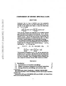
Definiton 2.23 (incomposable/decomposable) ([11], p. 395f ) A matrix M is called decomposable if it has (up to a permutation of the rows and columns) the following form � � B 0 M= C D where B and D are square matrices. Otherwise the matrix M is called indecomposable. The meaning of this definition is the following: We associate a directed graph GM to the matrix M such that there is a directed edge from i to j iff Mij > 0. Clearly, the matrix M is indecomposable iff the graph GM is strongly connected. We note that a symmetric matrix M is indecomposable iff the associated graph GM is connected. Example 2.24 Look at the following matrix M and the associated directed graph GM :
1 1 1 0 1 0 0 1 1 1
2
3
The matrix M is decomposable because of the the decomposition shown on the left. The graph GM is not strongly connected, because there is no (directed) path from 1 to 3. Theorem 2.25 (Perron-Frobenius) Suppose M is a real nonnegative indecomposable matrix. Then: 1. There exists a positive real simple eigenvalue of M and an associated eigenvector whose entries are all positive. Let λP F be such an eigenvalue. 24
2. All eigenvalues λ of M satisfy |λ| ≤ λP F , i.e. λP F is the largest eigenvalue (in absolute value). In particular λP F is unique. 3. If θ is an eigenvalue of M and |θ| = λP F , then θ/λP F is an mth root of unity and e2πir/m λP F is an eigenvalue of M for all r. Remark 2.26 i) A simple eigenvalue is an eigenvalue with multiplicity 1. ii) The eigenvalue λP F is called the Perron-Frobenius eigenvalue of M . iii) Let M be some real nonnegative symmetric indecomposable matrix and assume we have a positive eigenvector v for some eigenvalue λ. We claim that the eigenvalue λ is equal to the Perron-Frobenius eigenvalue. Otherwise assume λP F (A(G)) 6= λ. There is a positive eigenvector vP F corresponding to the Perron-Frobenius eigenvalue. Then v T vP F > 0, i.e. they are not orthogonal despite they correspond to different eigenvalues. Contradiction to Lemma 1.7. We will now look at some applications of Theorem 2.25 to spectral graph theory. The following lemma contains two statements which we know already. The first statement is one part from Lemma 2.5 and the second statement one part from Lemma 2.12. However, the method used here to derive the statement is another. Lemma 2.27 i) For d-regular graphs G on n vertices: |λi (A(G))| ≤ d,
1 ≤ i ≤ n.
If G is also connected then d is a simple eigenvalue. ii) For graphs G on n vertices: λi (L(G)) ≤ 2∆,
1 ≤ i ≤ n.
Proof: i) The adjacency matrix is real and nonnegative. W.l.o.g. we can assume that the graph G is connected. Then the adjacency matrix of G is also indecomposable. We know that the vector (1, 1, ..., 1)T is an eigenvector to the eigenvalue d. By the remark above, we know that λP F = d. The second part in the theorem gives us the desired inequality. ii) (Mohar [22], p.10) W.l.o.g. we can assume that the graph G is connected. Then the matrix M := ∆I − L(G), where I is the identity matrix, is real nonnegative and indecomposable. We know that the vector (1, 1, ..., 1)T is an eigenvector to the eigenvalue ∆ of M . By the remark above we have 25
λP F = ∆. Perron-Frobenius Theorem implies that ∆ is greater or equal than the absolute value of all the eigenvalues of M , i.e. ∆ ≥ |∆ − λi |. In particular, ∆ ≥ λi − ∆ as claimed. � The Perron-Frobenius Theorem 2.25 leads to a very interesting theorem that characterizes bipartite graphs by their adjacency spectrum: Theorem 2.28 (eigenvalues of bipartite graphs) ([4], p.178) Let G be a connected graph with adjacency matrix A and adjacency eigenvalues λ1 ≤ λ2 ≤ ... ≤ λn . Then the following are equivalent: 1. G is bipartite 2. The spectrum of the adjacency is symmetric about the origin, i.e. λi = −λn−i+1 , for all 1 ≤ i ≤ n. 3. λ1 = −λn . Proof: 1 =⇒ 2: Suppose G is bipartite. Then the adjacency matrix looks like this (perhaps after a permutation of the vertices): � � 0 B A= BT 0 where B is some square matrix. If the partitioned vector (x, y) is an eigenvector of A with eigenvalue θ, then (x, −y) is an eigenvector of A with eigenvalue −θ. This means that the spectrum is symmetric about the origin. 2 =⇒ 3: clear. 3 =⇒ 1: Suppose we have a graph with adjacency eigenvalues λi such that λn = −λ1 and let v and w denote an eigenvector to the eigenvalue λn and λ1 , respectively. These two eigenvectors are orthogonal by Lemma 1.7. The largest eigenvalue of A2 is λ21 = λ2n because of Lemma 1.5. If the matrix A2 has an Perron-Frobenius eigenvalue then it would be λ21 = λ2n . This eigenvalue is not simple because it has two linearly independent eigenvectors v, w. This would be a contradiction to the first point of the Perron-Frobenius Theorem. Since A2 is real and nonnegative it has to be decomposable. So we can write � � � � �2 � A21 + A2 AT2 A1 A2 B 0 A1 A2 + A 2 A3 2 = = A =: C D AT2 A3 AT2 A1 + A3 AT2 AT2 A2 + A23 Specially A1 A2 + A2 A3 = 0. Since G is connected we conclude that A2 6= 0. All these matrices are nonnegative matrices. Thus A1 = 0 and A3 = 0, i.e. G is bipartite. � 26
2.3
Trace of a Matrix
In this section we try to connect the trace of the three matrices A(G),L(G), and L(G) of a graph G to some of the properties/paramters of G. Then we can also relate these properties/parameters to the eigenvalues of G since by Lemma 1.6 the trace of a matrix is equal to the sum of its eigenvalues. First let us look at the adjacency: Lemma 2.29 ([4], p.165) Let G = (V, E) be a graph with adjacency eigenvalues λ1 , ..., λn . Then n X
j=1 n X
j=1 n X
λi = tr(A(G)) = 0, λ2i = tr(A2 (G)) = 2e, λ3i = tr(A3 (G)) = 6t;
j=1
where e is the number of edges and t is the number of triangles, formally t = |{{a, b, c} ∈ V 3 ; {a, b} ∈ E, {b, c} ∈ E, {c, a} ∈ E}|. There is a more general theorem about the number of walks in a graph which we will mention here: Theorem 2.30 (Number of Walks) ([4], p.165) Let G be a graph with adjacency matrix A(G). The number of walks from u to v in G with length r is (Ar )uv . By using Theorem 2.30 we can reprove some parts of Theorem 2.28: Theorem 2.31 The following are equivalent statements about a graph G on n vertices with adjacent eigenvalues λ1 ≤ ... ≤ λn . 1. G is bipartite 2. The adjacency spectrum is symmetric about the origin, i.e. λi = −λn−i+1 for all 1 ≤ i ≤ n. Proof: ([30], p.455) 1 =⇒ 2: See proof of Lemma 2.28. 27
2t−1 2 =⇒ 1: If λi = −λn−i+1 , then λi2t−1 = −λn−i+1 for every positive integer t. And n n X � 1 X 2t−1 2t−1 2t−1 = 0. λi + λn−i+1 λi = 2 i=1 i=1 P k Because λi counts the closed walks of length k in the graph (from each starting vertex), we get from the above equation, that G does not contain any closed walk of odd length. So G does not contain an odd cycle, since an odd cycle is an odd closed walk. Hence G is bipartite by Lemma 1.2. �
We will now look at the trace of the Laplacian: Lemma 2.32 Let G be a graph on n vertices with Laplacian L. Then n X
λ(L) = tr(L) = vol1 (G)
i=1 n X
λ2 (L) = tr(L2 ) = vol2 (G) + vol1 (G)
i=1
n X i=1
λ3 (L) = tr(L3 ) = vol3 (G) + 3 vol2 (G) − 6t.
where t is (again) the number of triangles in G and volk (G) =
n X
dki .
i=1
Proof: The diagonal elements of L are the degrees. Thus tr(L) =
n X
di = vol1 (G).
i=1
We will now calculate the matrix L2 . L2ij =
n X k=1
Lik Lkj = di Lij −
X
Lkj .
k:k∼i
By distinguish three different cases, we get: 2 if i = j; di + d i , −di − dj + codeg(i, j), if i ∼ j; L2ij = codeg(i, j), otherwise. 28
where codeg(i, j) is the codegree of i and j, i.e. the number of common neighbors. So we get 2
tr(L ) =
n X
d2i + di = vol2 (G) + vol1 (G).
i=1
Furthermore, the diagonal elements of L3 are L3ii
=
n X k=1
=
d3i
=
d3i
Lik L2kj = di L2ii −
+
d2i
+
d2i
+
X k∼i
X
L2ik
k:k∼i
di + dk − codeg(k, i) X
+ d2i +
k∼i
dk −
X
codeg(k, i)
k∼i
Finally 3
tr(L ) =
n X
L3ii
= vol3 (G) + 2 vol2 (G) +
n X X i=1 k∼i
k=1
|
{z
dk −
=vol2 (G)
}
n X X
i=1 k:k∼i
|
codeg(i, k) . {z
=6t
}
�
Lemma 2.33 Let G be a graph on n vertices with with normalized Laplacian L. Then n X
λi (L) = tr(L) = n
i=1
n X i=1
n X i=1
λ2i (L) = tr(L2 ) = n + e−1 (G, G)
(1 − λi (L))2 = tr((I − L)2 ) = e−1 (G, G)
where e−1 (G, G) =
n X X i=1
1 . d i dk k:k∼i
Proof: We calculate n X i=1
λ2i (L) = tr(L2 ) =
n n X X i=1 j=1
Lij Lji =
n X i=1
29
X 1 1+ dd j∼i i j
!
= n + e−1 (G, G).
And n X i=1
2
(1 − λi (L)) =
n X i=1
1−2
n X
λi (L) +
i=1
n X i=1
λi (L)2 = e−1 (G, G). �
Definiton 2.34 (strongly regular graph) A strongly regular graph with parameters (n, d, η, µ) is a d-regular graph on n vertices in which every pair of adjacent vertices has exactly η common neighbors and every pair of nonadjacent vertices has exactly µ common neighbors. Proposition 2.35 ([18], p.16) Let G be a connected strongly regular graph with parameters (n, d, η, µ). Then the adjacency eigenvalues of G are: λ1 = d with multiplicity s1 = 1 and � p 1� 2 η − µ ± (η − µ) + 4(d − µ) λ2,3 = 2
with multiplicities
s2,3
1 = 2
(n − 1)(µ − η) − 2d n−1± p (µ − η)2 + 4(d − µ)
!
.
Proof: We use Theorem 2.30 to compute the matrix A2 . The walks of length 2 from a vertex to itself must go over one of its neighbors. Thus we have d such walks. A walk of length 2 which connects two different vertices must go over one of theirs common neighbors. So we have η such walks for adjacent vertices and µ for non-adjacent vertices respectively. Altogether we can write: A2 = (d − µ)I + µJ + (η − µ)A, where J is the n × n all one matrix and I is the (n × n) identity matrix. We know that the vector w = (1, 1, ..., 1)T is an eigenvector of A associated with the eigenvalue d (see Lemma 2.5). Moreover, d is a simple eigenvalue because G is connected (see Perron-Frobenius Theorem). All other eigenvectors have to be orthogonal to w (see Lemma 1.7). Let v 6= 0 be an eigenvector with eigenvalue λ which is orthogonal to w, i.e. Jv = 0. Then λ2 v = A2 v = (d − µ)v + (η − µ)λv Since v 6= 0 we get
λ2 − (d − µ) − λ(η − µ) = 0. 30
This equation has two solution λ2 and λ3 as defined in the proposition formulation. If we denote by s2 and s3 the respective multiplicities of λ2 and λ3 , we get 1 + s2 + s3 = n,
tr(A) = d + s2 λ2 + s3 λ3 = 0.
Solving the above system of linear equations for s2 and s3 we obtain the assertion of the proposition. � Example 2.36 • The 5-cycle C5 is a strongly regular graph with parameters (5,2,0,1). So the eigenvalues of C5 are √ ![2] √ ![2] −1 + 5 −1 − 5 2, , . 2 2 • The Petersen graph is a strongly regular graph with paramters (10,3,0,1). So the eigenvalues are 3, 1[5] , −2[4] . Lemma 2.37 Let G be a graph on n vertices and normalized Laplacian eigenvalues λ1 , ..., λn−2 , x, y. Suppose we know all eigenvalues but two x, y. Then we can compute the remaining two eigenvalues in the following manner p 1 (α + 2β − α2 ) x = 2 p 1 y = (α − 2β − α2 ) 2
where
α = n−
n−2 X
λi
i=1
β = n + e−1 (G, G) −
n−2 X
λ2i .
i=1
Proof: We solve the following system of equations X λi + x + y = n X λ2i + x2 + y 2 = n + e−1 (G, G).
31
�
2.4
Eigenvectors
We will construct in this section some explicit eigenvectors for some special graphs. The first time we see a graph we can look for some special structures, e.g. twins, which will help us to determine some of the eigenvalues of the graph. Definiton 2.38 (twins) Two vertices i, j are called twins if for all other vertices k k ∼ i ⇐⇒ k ∼ j. Lemma 2.39 Let G be a graph and suppose there are two nonadjacent twin vertices i, j, i.e. N (i) = N (j). We define the (Faria) vector v as if k = i; 1, −1, if k = j; vk := 0, otherwise.
Then
1. λ = 0 is an eigenvalue of the adjacency with eigenvector v; 2. λ = di = dj is an eigenvalue of the Laplacian with eigenvector v; 3. λ = 1 is an eigenvalue of the normalized Laplacian with eigenvector v. Proof: We get X (Av)k = vl , l∼k
(Lv)k = dk vk −
X l∼k
vl ,
(Lv)k = vk −
X l∼k
√
vl . d k dl
Since any vertex k 6= i, j is either connected to both i and j or to none of them, we have (Av)k = (Lv)k = 0. We also obtain (Lv)k = 0 because di = dj . Clearly (Av)i = (Av)j = 0 since i and j are not adjacent. There remains two calculations: (Lv)i = di , (Lv)i = 1 and the same for j. � Lemma 2.40 Let G be a graph and suppose there are two adjacent twin vertices i, j, i.e. N (i) − {j} = N (j) − {i}. We define the (Faria) vector v as if k = i; 1, −1, if k = j; vk := 0, otherwise. Then
32
1. λ = −1 is an eigenvalue of the adjacency with eigenvector v; 2. λ = di + 1 = dj + 1 is an eigenvalue of the Laplacian with eigenvector v; dj +1 dj
3. λ = did+1 = i eigenvector v.
is an eigenvalue of the normalized Laplacian with
Proof: The proof is the same as in Lemma 2.39.
�
Example 2.41 We can now easily compute the normalized Laplacian eigenvalues of some special graphs: • The first example will be the complete graph Kn . Every pair of vertices are twins in the complete graph which are adjacent and have degree n − 1. By Lemma 2.40 each of these pairs is defining an eigenvector associated to the eigenvalue n/(n−1) but not all of them are linearly independent. We can chose the eigenvectors of the form (1, 0, ..., −1, ..., 0)T where the j th entry is -1 for all j from 2 to n. We get n-1 such eigenvectors associated to eigenvalue n/(n − 1) which are linearly independent. Also 0 is an eigenvalue with eigenvector (1, 1, ..., 1)T . So we have derived the whole normalized Laplacian spectrum of Kn . spec(L(Kn )) = 0,
�
n n−1
�[n−1]
.
• Second, we look at the star Sn with n vertices. Every pair of noncentered vertices are non-adjacent twins. By Lemma 2.39 each of these pairs is defining an eigenvector associated to the eigenvalue 1 but not all of them are linearly independent. We can chose the eigenvectors of the same form as above and get n − 2 linearly independent eigenvectors associated to the eigenvalue 1. Also 0 is an eigenvalue. We receive the last eigenvalue by looking at the trace (cf. Lemma 2.33). The sum of all eigenvalues is equal to n. So the last eigenvalue must be 2. spec(L(Sn )) = 0, 1[n−2] , 2. Example 2.42 We look at some graph G and glue a triangle in some vertex. The resulting graph is shown in the following picture:
33
x
G
y
Now from the Lemma 2.40 we know that this graph has a normalized Laplacian eigenvalue 3/2 with an eigenvector which assigns x to 1 and y to -1 and all other vertices to 0. This eigenvalue is determined locally. Next, we look at a generalization of the Lemma 2.39. Lemma 2.43 Suppose we have two disjoint subsets U+ and U− of the vertices such that |N (x) ∩ U+ | = |N (x) ∩ U− |,
∀x ∈ V.
This means that the number of neighbors of x in U+ is the same as the number of neighbors of x in U− for all vertices x (also for vertices in U+ and U− ). Then 1 is an eigenvalue of the normalized Laplacian with eigenvector √ dx , x ∈ U+ ; √ fx := − dx , x ∈ U − ; 0, otherwise. Proof: We consider first the following sum for any vertex x: p p X X fy X dy dy p p p = − dy dx dy dx y∼x,y∈U− dy dx y:y∼x y∼x,y∈U+ =
|N (x) ∩ U+ | |N (x) ∩ U− | √ √ − = 0. dx dx 34
So (Lf )x = fx −
f p y = fx . d y dx y:y∼x X
This means that 1 is an eigenvalue of L with eigenvector f .
�
Question: Are there other eigenvectors for the normalized Laplacian possible associated to the eigenvalue 1? - We don’t know. Definiton 2.44 (k-blow-up) Let G be a graph on n vertices. The k-blowup of G, denoted by G(k), is obtained by replacing each vertex of G by an independent set of size k and connecting two vertices of G(k) by an edge if and only if the corresponding vertices of G are connected by an edge. Lemma 2.45 Let G be a graph on n vertices with normalized Laplacian eigenvalues λ1 , ..., λn . Then the eigenvalues of the k-blow-up of G are 1 with multiplicity n(k − 1) and λ1 , ..., λn Proof: We will only sketch a proof. The eigenvalues 1 are derived via Lemma 2.39. There are n(k − 1) linearly independent eigenvectors of the form (. . . , 1, . . . , −1, . . .). Each eigenvalue of G is also an eigenvalue of G(k) since the eigenvector can be “blown up”. Finally we can check that we have enough eigenvalues n(k − 1) + n = nk. � Example 2.46 We can now compute the whole spectrum of the complete k-partite graph Km,...,m where n = km. We notice that Km,...,m is the mblow-up of the complete graph Kk . The normalized Laplacian spectrum of Kk is given by k [k−1] spec(L(Kk )) = 0, . k−1 By using the Lemma 2.45 we get the normalized Laplacian spectrum of Km,...,m k [k−1] [k(m−1)] . spec(L(Km,...,m )) = 0, 1 , k−1
We have also seen applications of the eigenvector-method in section 2.1: The vector (1, 1, ..., 1)T is an eigenvector of the adjacency of a d-regular graph and of the Laplacian of any graph. We can use the eigenvector-method for graphs with a special appearance as we have seen in this section. But for general graphs we can’t say much. 35
2.5
Rayleigh quotient
The Rayleigh quotients for the adjacency, Laplacian and normalized Laplacian of some graph G are P 2 i∼j xi xj Pn 2 (5) R(A; x) = i=1 xi P 2 i∼j (xi − xj ) Pn 2 R(L; x) = (6) i=1 xi P 2 i∼j (xi − xj ) Pn R(L; D−1/2 x) = . (7) 2 i=1 di xi
The Rayleigh-Ritz Theorem and also the Courant-Fisher Theorem give us the connection between the eigenvalues and the Rayleigh quotient. We can bound the eigenvalues of G by calculating the Rayleigh quotient for some vector x. So almost all of the time we will use the method as described in the following corollary of the Rayleigh-Ritz Theorem:
Corollary 2.47 Let G be a graph on n vertices with adjacency matrix A and Laplacian L and normalized Laplacian L. i) If f is any vector then λn (A) ≥ R(A; f ) ≥ λ1 (A), λn (L) ≥ R(L; f ) ≥ λ1 (L), λn (L) ≥ R(L; f ) ≥ λ1 (L). ii) If G is d-regular and f a vector which is orthogonal to (1, 1, ..., 1) T then λn−1 (A) ≥ R(A; f ) iii) If f is a vector which is orthogonal to (1, 1, ..., 1)T then R(L; f ) ≥ λ2 (L); R(L; f ) ≥ λ2 (L). Lemma 2.48 ([22], p.8) Let s, t ∈ V (G) be nonadjacent vertices of a graph G with Laplacian eigenvalues λ1 ≤ λ2 ≤ ... ≤ λn . Then 1 λ2 ≤ (ds + dt ). 2 36
Proof: Let f be the following vector v = s; 1, −1, v = t; fv : 0, otherwise.
Since f ⊥ 1, the Rayleigh-Ritz Theorem yields P 2 f T Lf ds + d t {u,v}∈E (fu − fv ) P λ2 ≤ T = . = 2 f f 2 v∈V fv
�
Lemma 2.49 ([6], p. 7) Let G = (V, E) be a connected graph on n vertices. Then the following statements are equivalent: 1. G is bipartite 2. The greatest normalized Laplacian eigenvalue is 2, i.e. λn (L(G)) = 2. Proof: 1 =⇒ 2: Let A, B be the partite sets. Define the vector � 1, if i ∈ A; fi = −1, if i ∈ B. Then we have R(L; D
1/2
f) =
P
− f j )2 4e(A, B) P = = 2. 2 2|E| i d i fi
i∼j (fi
We conclude that this is the maximum of the Rayleigh quotient by Lemma 2.18. The Rayleigh-Ritz Theorem give us that λn (L(G)) = 2. 2 =⇒ 1: Let x 6= 0 be the vector where the Rayleigh quotient R(L; ·) takes its maximum which is 2. Then for y = D 1/2 x P P 2 2 2 (y − y ) i j i∼j i∼j 2yi + 2yj −1/2 P P 2 = R(L; x) = R(L; D y) = ≤ = 2. 2 2 i d i yi i d i yi We conclude that in the above equation there has to be always equality signs. Thus if i ∼ j then yi2 − 2yi yj + yj2 = (yi − yj )2 = 2yi2 + 2yj2 . 37
This is equivalent to yi = −yj whenever i ∼ j. Since G is connected and y 6= 0 none of the coordinate yi is zero. We define now a partition of the vertices into a set where yi > 0 and another set where yi < 0. By the condition yi = −yj there can be no edges within a part, i.e. G is bipartite. � In the beginning we have seen that λn ≥ n/(n − 1) (Lemma 2.18). Since all graphs are n-colorable this is a special case of the following Lemma. Lemma 2.50 Let G be a graph on n vertices with normalized Laplacian k . eigenvalues 0 = λ1 ≤ λ2 ≤ ... ≤ λn . If G is k-colorable, then λn ≥ k−1 Proof: Let us denote the different parts of G by A, B, C1 , ..., Ck−2 such that the number of edges between A and B, denoted by e(A, B), is maximal, i.e. e(A, B) = max{e(A, B), ..., e(A, Cj ), ..., e(B, Cj ), ..., e(Ci , Cj ), ...}. Look at the vector
if v ∈ A; 1, −1, if v ∈ B; fv := 0, otherwise.
Then λn ≥ R(L; D =
1/2
f) =
4e(A, B) + 2e(A, B) +
P
Pk−2
i=1 Pk−2
− f w )2 2 v fv d v
(f u∼w P u
e(A, Ci ) + e(B, Ci )
e(A, Ci ) + e(B, Ci ) P e(A, Ci ) + e(B, Ci ) k (4k − 4)e(A, B) + (k − 1) k−2 = Pk−2 i=1 k−1 2ke(A, B) + k i=1 e(A, Ci ) + e(B, Ci ) P k 2ke(A, B) + k k−2 k i=1 e(A, Ci ) + e(B, Ci ) ≥ = . Pk−2 k − 1 2ke(A, B) + k i=1 e(A, Ci ) + e(B, Ci ) k−1 i=1
�
Remark 2.51 i) The bound in Lemma 2.50 is sharp. Let us look at the k-partite graphs with parts of equal size. In Example 2.46 we have seen that the largest normalized Laplacian eigenvalue is k/(k − 1). ii) We note that Lemma 2.50 is a special case of Theorem 6.7 in Chung’s book [6]. 38
2.6 2.6.1
Interlacing Interlacing Theorems
If M is real symmetric n × n matrix, let λ1 (M ) ≤ λ2 (M ) ≤ ... ≤ λn (M ) denote the eigenvalues in nondecreasing order. The principal submatrices are obtained from M by deleting some rows and the columns with the same indices. Choose any subset J ⊆ {1, 2, ..., n}, then the principal submatrix of M indexed by J is the |J| × |J| matrix which can be written as (Mij )i∈J,j∈J . Theorem 2.52 (Interlacing) ([4], p.193) Let A be a real symmetric n×n matrix and let B be a principal submatrix of A with order m × m. Then, for i = 1, ..., m, λi (A) ≤ λi (B) ≤ λi+n−m (A). Note: We have the opposite order as in Godsil. Theorem 2.53 (Interlacing for the adjacency matrix) Let G be a graph on n vertices and let v ∈ V . Denote H = G − v to be the induced subgraph of G without the vertex v. Then λi (A(G)) ≤ λi (A(H)) ≤ λi+1 (A(G)). Proof: The adjacency matrix of H = G − v is a principal submatrix of the adjacency matrix of G. So by using the Theorem 2.52 we get the desired inequalities. � Definiton 2.54 (interlace) The sequence µ1 , . . . , µn−1 interlace the sequence λ1 , . . . , λn if for 1 ≤ k ≤ n − 1 we have λk ≤ µk ≤ λk+1 . Example 2.55 We look at the 5-cycle G = C5 . By deleting one vertex of C5 we obtain a path with 3 edges, i.e. H = P3 . The adjacency eigenvalues of C5 are √ √ √ √ −1 − 5 −1 − 5 −1 + 5 −1 + 5 , , , , 2. 2 2 2 2 By the Theorem 2.53 we know that the adjacency eigenvalues of P3 (say λ1 ≤ . . . ≤ λ4 ) interlace the adjacency eigenvalues of C5 , i.e. √ √ √ √ −1 − 5 −1 + 5 −1 + 5 −1 − 5 ≤ λ1 ≤ ≤ λ2 ≤ ≤ λ3 ≤ ≤ λ4 ≤ 2 2 2 2 2 39
√
√
Thus λ1 = −1−2 5 and λ3 = −1+2 5 are eigenvalues of P4 . The remaining two eigenvalues are bounded from above and below. Indeed the eigenvalues of P3 can be calculated as √ √ √ √ −1 − 5 1 − 5 −1 + 5 1 + 5 , , , . 2 2 2 2 Remark 2.56 The same theorem for the Laplacian or the normalized Laplacian cannot be true. The point is the following. If we delete a vertex v from a graph then in the adjacency matrix we have to delete a column and a row but the other entries will remain the same. However, in the Laplacian the rows and columns corresponding to neighbors of v will also change. We can look at the following example. Let G = Kn . The Laplacian and normalized Laplacian eigenvalues of Kn are spec(L(Kn )) = 0, n[n−1] n [n−1] . spec(L(Kn )) = 0, n−1 So the Laplacian eigenvalues of Kn do not interlace the Laplacian eigenvalues of Kn+1 . Also the normalized Laplacian eigenvalues of Kn do not interlace the normalized Laplacian eigenvalues of Kn+1 . Nevertheless, we can state another interlacing theorem for the Laplacian: Theorem 2.57 (Interlacing for the Laplacian) ([4], p.291) Let G be a graph on n vertices and let H = G − e be a subgraph of G obtained by deleting an edge in G. Then the n − 1 smallest Laplacian eigenvalues of G interlace the Laplacian eigenvalues of H, i.e. for all 1 ≤ k ≤ n − 1 λk (L(G − e)) ≤ λk (L(G)) ≤ λk+1 (L(G − e)). Furthermore λn (L(G − e)) ≤ λn (L(G)). Example 2.58 We look at the 4-cycle, i.e. G = C4 , which has Laplacian eigenvalues 0, 2, 2, 4. By deleting an edge we get a path with 3 edges, i.e. H = P3 . We denote the Laplacian eigenvalues of H by λ1 ≤ . . . ≤ λ4 . Theorem 2.57 give us now λ1 ≤ 0 ≤ λ 2 ≤ 2 ≤ λ 3 ≤ 2 ≤ λ 4 ≤ 4 Indeed, the Laplacian eigenvalues of P4 are √ λ1 = 0, λ2 = 2 − 2, λ3 = 2,
λ4 = 2 +
√
2.
Question: Can we state Theorem 2.57 also for the normalized Laplacian? 40
2.6.2
Interlacing for Independent Set
Corollary 2.59 ([16], p.88) Let G be a graph on n vertices with maximal degree ∆. For a set I, the number of eigenvalues of A(G) that fall inside I (counting multiplicites) is denoted by aG (I). Then the independent number α(G) satisfies: α(G) ≤ aG ([0, ∆]); α(G) ≤ aG ([−∆, 0]). Proof: Let B be the principal submatrix of A(G) indexed by the α(G) vertices that belongs to some maximum independent set in G. Clearly, B is the zero matrix, i.e. all eigenvalues are zero. By the Interlacing Theorem 2.52 we conclude λα(G) (A(G)) ≤ 0 ≤ λn−α(G)+1 (A(G)) i.e. there are at least α(G) eigenvalues which are negative or zero and there are at least α(G) eigenvalues which are positive or zero. � Corollary 2.60 ([12], p.21) Let G be a graph on n vertices. For a set I, the number of eigenvalues of L(G) that fall inside I (counting multiplicites) is denoted by mG (I). Then α(G) ≤ mG ([δ, 2∆]); α(G) ≤ mG ([0, ∆]). Proof: First we note that all the eigenvalues lie in the interval [0, 2∆] (Lemma 2.12). Let B be the principal submatrix of L(G) indexed by the α(G) vertices that belongs to some maximum independent set in G. Clearly, B is a diagonal matrix of whose eigenvalues lie between δ and ∆. By the Interlacing Theorem 2.52 we conclude λα(G) (L(G)) ≤ λα(G) (B) ≤ ∆ and λn−α(G)+1 (L(G)) ≥ λn−α(G)+1 (B) ≥ δ. So there are at least α(G) eigenvalues in the interval [0, ∆] and there are at least α(G) eigenvalues in the interval [δ, 2∆]. � 41
2.6.3
Interlacing for Hamiltonicity
Proposition 2.61 ([4], p.195 and p.291) The Petersen graph P has no Hamiltonian cycle. Proof: We will prove this statement indirect. Assumption: P contains an Hamiltonian cycle. So after deleting some edges in P we will get C10 . Then by the Interlacing Theorem for the Laplacian 2.57 we get λk (L(C10 )) ≤ λk (L(P )),
1 ≤ k ≤ 10.
(8)
The Petersen graph P is strongly regular and has adjacency eigenvalues 3, 1[5] , −2[4] (Example 2.36). Thus, by using Lemma 2.20 the Laplacian spectrum of P is: 0, 2[5] , 5[4] . The Laplacian spectrum of C10 is √ ![2] √ ![2] √ ![2] √ ![2] 1− 5 1− 5 1+ 5 1+ 5 , 2+ , 2− , 2+ , 4. 0, 2 − 2 2 2 2 We note that √ 1− 5 λ6 (C10 ) = 2 − = 2.618... > 2 = λ6 (P ). 2 This is a contradiction to (8). Thus the assumption was wrong and the statement is proven. �
2.7
Gerschgorin’s Theorem
Theorem 2.62 (Gerschgorin) ([11], p.464) Let A = (aij )ij be a complex matrix. Let λ be an eigenvalue of A. Then X |akk − λ| ≤ |akj |. j:j6=k
for some k ∈ {1, . . . , n}, i.e. the spectrum of the matrix is contained in the union of these discs. 42
Proof: Since λ is an eigenvalue, there is an eigenvector x 6= 0 such that Ax = λx or equivalent (A − λI)x = 0. Let k be an integer such that |xk | = maxi |xi |. Then X X X |akj ||xj | ≤ |xk | |akj |. akj xj ≤ |akk − λ||xk | = j:j6=k
j:j6=k
j:j6=k
By dividing through |xk | we get our result.
�
We apply Gerschgorin’s Theorem to the adjacency matrix. Since all diagonal entries of the adjacency matrix are zero we get |0 − λ(A(G))| ≤
X
j:j6=k
|A(G)kj | = dk
for some k. Thus we can conclude that the adjacency eigenvalues take place in the interval [−∆, ∆]. This is one part of Lemma 2.4. Also we can deduce the corresponding parts in Lemma 2.12 and 2.18. But in fact the prove of these lemmas is an imitation of the above proof. Example 2.63 We look at the path of length 2, i.e. G = P2 :
1 −1 0 L := L(G) = −1 2 −1 0 −1 1
We conclude by using Gerschgorin’s Theorem that all the eigenvalues 0 = λ1 , λ2 , λ3 are in the interval [0,4] but this says nothing more than Lemma 2.12. So we try to get a better statement. For this we “subtract” the eigenvector v := (1, 1, 1)T which belongs to the eigenvalue λ1 = 0, i.e. we look at
2 0 1 L + vv T = 0 3 0 1 0 2 The eigenvector v = (1, 1, 1)T belongs in L to 0 and in L+vv T to 3. All other eigenvectors of L are orthogonal to v, i.e. v T v = 0 (Lemma 1.7 and PerronFrobenius Theorem). Thus they are also eigenvectors of L + vv T associated with the same eigenvalue as in L. Gerschgorin’s Theorem give us now, that the λ1 and λ2 are in the interval [1,3]. 43
2.8
Majorization
We refer to the book ”Inequalities: Theory of Majorization and Its Applications” [1] for more information about the theory of Majorization and there especially chapter 9. Also Johnson [26] contains a section about majorization but with small differences in the formulations. Definiton 2.64 (decreasing rearrangement) For any x = (x1 , ..., xn ) ∈ Rn , let x[1] ≥ ... ≥ x[n] denote the components of x in decreasing order. Let (x[1] , ..., x[n] ) be called the decreasing rearrangement of x. Definiton 2.65 (majorize) The vector x is said to majorize the vector y if the following two conditions hold: i X k=1
n X k=1
x[k] ≥ x[k] =
i X
y[k] ,
k=1
n X
for all 1 ≤ i ≤ n − 1,
and
y[k] .
k=1
Theorem 2.66 (Schur’s Majorization Theorem) Let A be a symmetric matrix. The vector of eigenvalues of A majorizes the vector of the diagonal entries of A. Corollary 2.67 Let G be a graph on n vertices with Laplacian eigenvalues λ1 ≤ λ2 ≤ ... ≤ λn . Suppose the degrees of G are ordered, i.e. δ = d1 ≤ ... ≤ dn = ∆. Then λn ≥ dn = ∆, λn + λn−1 ≥ dn + dn−1 .. . λn + . . . + λ 2 ≥ d n + . . . d 2
λ1 + . . . λn−1 ≤ d1 + . . . + dn−1 λ1 + . . . λn−2 ≤ d1 + . . . + dn−2 .. . λ1 ≤ d 1 = δ
And λn + . . . + λ 1 = d n + . . . + d 1 . 44
Remark 2.68 The last equality which appears in the above corollary is the fact that the trace of a symmetric matrix is equal to the sum of its eigenvalues (see also Lemma 1.6). With this equality you can always change between the two equivalent form of the inequalities. The first form is written on the left and the second form is written on the right.
2.9
Miscellaneous
The determinant of the Laplacian and of the normalized Laplacian is always zero because λ = 0 is always an eigenvalue. However the determinant of the adjacency matrix is more interesting. There exists a theorem which connects the determinant of the adjacency matrix to some graph properties (see Harary [13], or Biggs [3], p.40f). A very similar definition to the determinant is the permanent. The permanent of the adjacency matrix of a bipartite graph counts the number of perfect matchings in it ([14]). The number of spanning trees is determined by the Laplacian (e.g. [4], p.281).
45
46
Chapter 3 Cauchy-Schwarz and other Inequalities 3.1
Cauchy-Schwarz Inequalitiy
The following inequality is known as Cauchy’s or Cauchy-Schwarz’s or CauchyBunyakovsky-Schwarz’s inequality: Theorem 3.1 (Cauchy-Schwarz inequality) ([9]) If a1 , ..., an and b1 , ..., bn are sequences of real numbers, then !2 n n n X X X 2 ≤ ak b k ak b2k k=1
k=1
k=1
with equality if and only if the sequences are proportional, i.e. there is an r ∈ R such that ak = rbk for each 1 ≤ k ≤ n. Proof: We calculate the difference between the left hand side (LHS) and the right hand side (RHS) and use Lagrange’s identity LHS − RHS =
n X k=1
a2k
n X k=1
b2k
−
n X k=1
ak b k
!2
n
n
1 XX (ai bj − aj bi )2 = 2 i=1 j=1
Since a sum of squares is always nonnegative we have proved the inequality, i.e. RHS ≥ LHS. Equality holds iff each of the above summands is zero, i.e. (ai bj − aj bi )2 = 0 47
for any 1 ≤ i, j ≤ n. We have to show now that in this case the sequences are proportional. If all bk = 0 then they are proportional with r = 0. Otherwise we chose bl 6= 0 and define r = al /bl . Then ak =
ak al bl = bk = rbk bl bl
Here we have used ak bl = al bk .
3.2
�
An inequality
In Chung’s paper ([7], p. 7) there is mentioned an inequality which she called a general Cauchy-Schwarz Inequality. We will state here this inequality in a more general way and give three different proofs, namely an elementary proof, a proof by using the Chebychev-inequality and finally a proof by using some general Cauchy-Schwarz-inequality. Lemma 3.2 For positive numbers aj > 0 and for α ≤ β + 1 the following inequality holds: k X
aαj
j=1
·
k X
aβj
≤
j=1
k X
aα−1 j
j=1
·
k X
aβ+1 . j
j=1
Proof: Let us first calculate the difference between the right hand side (RHS) and the left hand side (LHS):
RHS − LHS = =
k X
aα−1 j
j=1
k X
·
k X
aβ+1 j
j=1
aα−1 aβ+1 + j j
j=1
=
X
X
1≤i 1/2 the probability of a graph G1 with more edges than another graph G2 is higher. (And the probability of G1 is smaller than the probability of G2 if p < 1/2.) A lot of properties hold for almost all G ∈ G(n, p). We say that “the random graph G(n, p) has property P ” and mean that the probability of G ∈ G(n, p) 55
has property P tends to one as n tends to infinity. The following definition and theorem are concerned about the edge distribution of random graphs. Definiton 4.2 (e(U, W )) The number of edges between two disjoint subsets U, W of vertices is denoted by e(U, W ). More generally, we define X X e(U, W ) := 1. u∈U v∈V :u∼v
We note, that if we have an edge e with both endpoints in U ∩ W then this edge is counted twice in e(U, W ). Theorem 4.3 (random graph: edge distribution) ([18], p.4) Let p = p(n) ≤ 0.9. Then for every two (not necessarily disjoint) subsets U, W of vertices p |e(U, W ) − p|U ||W || = O( |U ||W |np)
for almost all G ∈ G(n, p).
The expected degree of a vertex v in a random graph G(n, p) is the same for all v. We consider in the following an extended random graph model for a general degree distribution. Definiton 4.4 (random graph with given degree distribution) Given w = (w1 , w2 , ..., wn ) a sequence. A random graph with given degree distribution G(w) is a probability space of all labeled graphs on n vertices {1, 2, ..., n}, where {i, j} is an edge of G(w) with probability wi wj ρ, independently of any other edges, for P 1 ≤ i ≤ j ≤ n where ρ plays the role of a normalization factor, i.e. ρ = ( ni=1 wi )−1 .
The expected degree of the vertex i is wi . The classical random graph G(n, p) can be viewed as a special case of G(w) by taking w to be the vector (pn, pn, ..., pn). Notice that we allow loops in this model but their presence does not play any essential role. The above definition of a random graph with given degree distribution comes from Chung und Lu [10]. There are also other definitions for random graphs with given degrees (see e.g. [17]).
4.2
Basics about Pseudo-random graphs
What are now pseudo-random graphs? Certainly, we don’t want to say that these are graphs which are more probably by the above probability distributions on graphs than others. But we want that pseudo-random graphs “behave” like random graphs, i.e. that a pseudo-random graph on n vertices 56
have (almost) the same properties than a random graph G(n, p) for some suitable p. Random graphs share a lot of properties. But the most fundamental thing that a graph consists is its edge distribution. So we define pseudo-randomness by consulting Theorem 4.3. The more the edge distribution of some graph (or rather of a family of graphs) looks like in Theorem 4.3, the more pseudorandom is this graph for us. If we know the eigenvalues of a graph G then we can make some statements about the edge-distribution of G. This will be our link to spectral graph theory. In the following we will define the concept of pseudo-random graphs by means of the eigenvalues of a graph. Definiton 4.5 (second adjacency eigenvalue) The second adjacency eigenvalue λ(A(G)) is defined as λ(A(G)) := max{−λ1 (A(G)), λn−1 (A(G))} = max |λi (A(G))|. i6=n
Definiton 4.6 ((n, d, λ)-graph) A (n, d, λ)-graph is a d-regular graph on n vertices with second adjacency eigenvalue at most λ. Theorem 4.7 ((n, d, λ)-graph: edge distribution) ([23], chapter 9) Let G be a (n, d, λ)-graph. Then for every two subsets B, C of vertices, we have p d|B||C| e(B, C) − ≤ λ |B||C|. n
If for a graph G the second adjacency eigenvalue λ(A(G)) is small then the edge distribution of G is (almost) the same as for the random graph G(n, d/n) by the above theorem. So in this sense the graph G is pseudo-random. To prove Theorem 4.7 we will use the following proposition. Proposition 4.8 ([23], Chapter 9) Let G = (V, E) be a (n, d, λ)-graph. Then for every subset B of V X� v∈V
|B|d |NB (v)| − n
�2
≤ λ2
|B|(n − |B|) n
where NB (v) denotes the set of all neighbors in B of v. 57
Proof: Define the vector f �
fv :=
1 − |B|/n, if v ∈ B; −|B|/n, otherwise.
This vector f is orthogonal to the 1 = (1, 1, ..., 1)T vector. Recall λ = max |λi (A(G))|
(Cor. 3.16)
=
i6=n
where Φ0 =
√1 (1, . . . , 1)T . n
Therefore
(f ⊥1)
(Af )T · (Af )
kA − dΦ0 ΦT0 k2
=
(C.S.)
≤ ≤ =
((A − dΦ0 ΦT0 )f )T · ((A − dΦ0 ΦT0 )f ) k(A − dΦ0 ΦT0 )f k2 kA − dΦ0 ΦT0 k22 kf k2 λ2 kf k2 .
On one side we get kf k2 = |B|(1 − |B|/n)2 + (n − |B|)(|B|/n)2 =
|B|(n − |B|) . n
On the other side (Af )T · (Af ) =
X ((1 − |B|/n)|NB (v)| − |B|/n(d − |NB (v)|))2 v∈V
X (|NB (v)| − |B|d/n)2 . = v∈V
The desired result follows.
�
Proof: Proposition 4.8 implies Theorem 4.7 By Theorem 4.8, X� v∈C
d|B| |NB (v)| − n
�2
≤
X� v∈V
d|B| |NB (v)| − n
�2
≤ λ2
|B|(n − |B|) . n
We can write the number of edges between B and C in the following form: e(B, C) =
X v∈C
58
|NB (v)|.
Thus, by the triangle inequality and the Cauchy-Schwarz inequality X d|B||C| d|B| e(B, C) − ≤ 1 · |NB (v)| − n n v∈C v u �2 X� (C.S.) u d|B| |NB (v)| − ≤ t|C| · n v∈C r p |B|(n − |B|) ≤ λ |C| ≤ λ |B||C|. n
�
There is a generalization of Theorem 4.7 with an improved “error term”. Theorem 4.9 ((n, d, λ)-graph: edge distribution) ([18], p.11) Let G be a (n, d, λ)-graph. Then for every two subsets U, W ⊆ V , s � �� � d|U ||W | |W | e(U, W ) − ≤ λ |U ||W | 1 − |U | 1− . n n n
So the second adjacency eigenvalue of a graph G is a measure of the pseudorandomness of G. If a graph has a very small second adjacency eigenvalue than it is very pseudo-random. How small can λ be? We answer this question in the following lemma. Lemma 4.10 (cf. [19], Prop. 2.3) Let G be a d-regular graph on n vertices with adjacency eigenvalues λ1 ≤ . . . ≤ λn . Then r d(n − d) . λ := max |λi | ≥ i6=n n−1 In particular, if d ≤ 0.9n then
√ λ = Ω( d)
as n → ∞.
Proof: Using Lemma 2.29 and the fact that λn = d (Lemma 2.5) we get: 2
nd = 2e = tr(A ) =
n X i=1
λ2i ≤ d2 + (n − 1)λ2 .
Solving the above inequality for λ establishes the claim of the lemma.
59
�
Example 4.11 i) Can we give an example of a pseudo-random graph? - We look at the complete graph Kn . By using Example 2.41 and Theorem 2.20 we get spec(A(Kn )) = −1[n−1] , n − 1. Thus the second adjacency eigenvalue 1. So Kn is very pseudo-random. Nevertheless, we notice that the quotient of the degree and the size of Kn tends to one, i.e. d(Kn )/n = (n − 1)/n → 1. So, the condition on Lemma 4.10 is not fulfills. ii) A famous pseudo-random graph is the Payley Pq graph ([18], p.17f) which has q vertices and is (q − 1)/2-regular. In fact, it can be calculated that the Pq is a strongly regular graph with parameters (q, q−1 , q−5 , q−1 ). By Lemma 2 4 4 √ 2.35 the second adjacency eigenvalue of Pq equals ( q + 1)/2. So this graph √ shows that the bound λ(G) = Ω( d) from the Lemma 4.10 is sharp. So far, we have defined the concept of pseudo-random regular graphs. We will extend it for non-regular graphs by looking at the normalized Laplacian eigenvalues. Our proceeding will be analogue to the regular case. Definiton 4.12 (second Laplacian eigenvalue) The second Laplacian eigenvalue is defined as λ(L(G)) := max |1 − λi (L(G))| = max{λn (L(G)) − 1, 1 − λ2 (L(G))}. i6=1
If all the normalized Laplacian eigenvalues, except λ1 = 0, are near 1, i.e. the second Laplacian eigenvalue is small, then we will see that the graph is a good pseudo-random graph. First, we note that the second Laplacian eigenvalue of a regular graph is the same as the second adjacency eigenvalue up some factor. Lemma 4.13 Let G be a d-regular graph. Then the second adjacency eigenvalue is d times the second Laplacian eigenvalue, i.e. λ(A(G)) = d · λ(L(G)). Proof: This is an immediate consequence of Lemma 2.20.
�
Definiton 4.14 (volume) The volume of a subset U of the vertices is defined as X vol(U ) := dj . j∈U
Note the abbreviated notation vol(G) := vol(V (G)). 60
Theorem 4.15 (second Laplacian eigenvalue: edge-distribution) ([6], p.72) Let G be a graph on n vertices with normalized Laplacian L and second Laplacian eigenvalue λ. Then for any two subsets X and Y of vertices p e(X, Y ) − vol(X) vol(Y ) ≤ λ vol(X) vol(Y ). vol(G) Proof: We define the characteristic vectors Φ(X) and Φ(Y ) by � � 1, i ∈ X; 1, i ∈ Y ; φ(X)i := φ(Y )i := 0, otherwise. 0, otherwise.
We have e(X, Y ) = φ(X)T Aφ(Y ) = φ(X)T D1/2 (I − L)D 1/2 φ(Y ). We remember λ = max |1 − λi (L)| i6=1
where Φ0 = √D
1/2 1
vol(G)
|e(X, Y ) −
(Cor. 3.16)
=
kI − L − Φ0 ΦT0 k2
. Therefore
vol(X) vol(Y ) | vol(G)
= (C.S.)
≤ ≤ =
|φ(X)T D1/2 · (I − L − Φ0 ΦT0 )D1/2 φ(Y )| kD1/2 φ(X)k2 k(I − L − Φ0 ΦT0 )D1/2 φ(Y )k2 kD1/2 φ(X)k2 kI − L − Φ0 ΦT0 k2 kD1/2 φ(Y )k2 p p vol(X)λ vol(Y ). �
There is a slightly stronger result: Theorem 4.16 (second Laplacian eigenvalue: edge-distribution) ([6], p.73) Let G = (V, E) be a graph on n vertices with second Laplacian eigenvalue λ. Suppose X, Y are two subsets of the vertices. Then p ¯ ¯ vol(X) vol(Y ) e(X, Y ) − ≤ λ vol(X) vol(Y ) vol(X) vol(Y ) vol(G) vol(G) ¯ (Y¯ ) denotes the complement of X (Y ), i.e. X ¯ = V \ X. where X 61
So the second Laplacian eigenvalue of a graph G is a measure of the pseudorandomness of G. If a graph has a very small second Laplacian eigenvalue than it is very pseudo-random. How small can λ be? We answer this question in the following lemma. Lemma 4.17 Let G be a graph on n vertices with normalized Laplacian L and second Laplacian eigenvalue λ. Then r e−1 (G, G) − 1 λ = max |1 − λi (L)| ≥ . i6=1 n−1 where e−1 (G, G) = In particular, if ∆ ≤ 0.9n then
n X X i=1
1 . d i dk k:k∼i
1 λ = Ω( √ ). ∆ Proof: Using Lemma 2.33 and the fact λ1 (L) = 0 we get e−1 (G, G) =
n X
(1−λi (L))2 = 1+
i=1
n X i=2
(1−λi (L))2 ≤ 1+
n X
λ2 = 1+(n−1)λ2 .
i=2
Solving the above inequality for λ establishes the first part of the claim of the lemma. We assume now ∆ ≤ 0.9n. Then e−1 (G, G) = Thus λ≥
n X n X X n 1 1 1 ≥ = = . di dk d∆ ∆ ∆ i=1 k:k∼i i i=1 k:k∼i
n X X i=1
r
e−1 (G, G) − 1 ≥ n
This proves the lemma.
r
n−∆ ≥ ∆n
r
0.1 . ∆ �
Example 4.18 We will look now at some (not regular) graphs and decide if they are pseudo-random or not. 62
• Let Ka be the complete graph on a vertices. We add k new vertices (without any edges) and then we connect each of these new vertices to all vertices of Ka . We denote the so-constructed graph by G. The number of vertices of G is a + k. Two vertices of Ka in G are adjacent twins with degree a+k −1 and two vertices of the new vertices in G are non-adjacent twins. By using Lemma 2.39 and Lemma 2.40 we conclude that G has the normalized Laplacian eigenvalues 1 with multiplicity a+k with multiplicity a−1. Also 0 is a normalized Laplacian k−1 and a+k−1 eigenvalue. Totally, we have found a + k − 1 eigenvalues so far. So there is one eigenvalue left. We calculate this eigenvalue by using the fact that the sum of all normalized Laplacian eigenvalues is equal to n (Lemma 2.33). Thus the last eigenvalue must be a+2k−1 . We summarize this by a+k−1 a + k [a−1] a + 2k − 1 , spec(L(G)) = 0, 1 , a+k−1 a+k−1 Thus G (or rather some family of such graphs) is a pseudo-random graph. Though, we notice that the maximum degree is in order of the number of edges such that we cannot apply Lemma 4.17. [k−1]
• Let G be any graph and we construct the graph H by gluing a triangle at one vertex of G. In Example 2.42 we have drawn a picture of this graph. Also we have seen that H has always an eigenvalue equal to 3/2. This means that the second Laplacian eigenvalue of H is at least 1/2, i.e. H is not at all pseudo-random. So, we can destroy the property of pseudo-randomness by this changes. So in this case the pseudorandomness is determined locally.
4.3
Edge Connectivity
Proposition 4.19 ([18], p.25) Let G be an (n, d, λ)-graph with d − λ ≥ 2. Then G is d-edge-connected. When n is even, it has a perfect matching. Proof: We will only prove the second statement by using Tutte’s condition (cf. Theorem 1.4). Since n is even, we need to prove that for every nonempty set S of vertices the induced graph G[V − S] has at most |S| connected components of odd size. From the first point of the statement, we know that G is d-edge-connected, so ¯ ≥ γd e(S, S)
where γ is the number of components in G[V − S]. On the other hand there are at most d|S| edges incident with vertices in S: ¯ ≤ d|S|. e(S, S) 63
Therefore G[V − S] has at most |S| connected components and hence G contains a perfect matching. � Definiton 4.20 (d¯U ) Let G = (V, E) be a graph. Then we write P di vol(U ) = u∈U . d¯U := |U | |U |
for the average degree of some set U ⊆ V . We write d¯ if we mean d¯V .
Lemma 4.21 Let U be a subset of vertices. Then δ ≤ d¯U ≤ ∆. Proof: We get: vol(U ) = d¯U = |U |
P
u∈U
|U |
du
≤
P
u∈U
|U |
∆
= ∆.
In fact, ∆ is the maximum of all of the average degrees d¯U . We bound each degree by the minimum degree and get the lower bound. � Clearly, we have vol(U ) = |U |d¯U . Thus we can rewrite the Theorem 4.15 in the following form q ¯ ¯ e(X, Y ) − dX |X|dY |Y | ≤ λ d¯X |X|d¯Y |Y | ¯ dn
where G = (V, E) is a graph on n vertices with second Laplacian eigenvalue λ and X, Y ⊆ V .
Theorem 4.22 (δ-edge-connected) Let G be a graph on n vertices with second Laplacian eigenvalue λ and minimum degree δ such that δ(1 − λ) ≥ 2. Then G is δ-edge-connected, even κ0 (G) = δ. Proof: Let U ⊆ V (G) with |U | ≤ n/2. We want to show that there are at least δ edges between U and U¯ . Case 1: 1 ≤ |U | ≤ d¯U =
vol(U ) . |U |
e(U, U¯ ) =
X v∈U
dv − e(U, U )
≥ |U |d¯U − |U |(|U | − 1) = |U |(d¯U − |U | + 1) ≥ d¯U ≥ δ. 64
Case 2: d¯U ≤ |U | ≤ n/2. Here we used the Theorem 4.16. d¯U |U |d¯U¯ (n − |U |) d¯U |U |d¯U¯ (n − |U |) − λ e(U, U¯ ) ≥ ¯ ¯ dn dn d¯U d¯U¯ |U |(n − |U |) = · · (1 − λ) n d¯ 1 d¯U d¯U¯ (1 − λ) · ≥ · |U | 2 d¯ Now we will look closer at the fraction
d¯U d¯U¯ . d¯
Note ¯
) U) ¯) |U | vol(U + (n − |U |) vol( vol(G) vol(U ) + vol( U |U | n−|U | d¯ = = = n� n � n vol(U ) vol(U¯ ) ≤ max = max{d¯U , d¯U¯ }. , |U | n − |U |
Thus e(U, U¯ )
|U | d¯U d¯U¯ (1 − λ) ¯ ¯ 2 max{dU , dU¯ } |U | δ(1 − λ) 2
≥ ≥ (cond.)
≥
|U | ≥ d¯U ≥ δ.
So this shows κ0 (G) ≥ δ. To get equality, we take a vertex v such that dv = δ and delete all edges from v (see also Whitney’s Theorem 1.3). � Remark 4.23 i) It is not obvious for us how to obtain some theorem about perfect matching by using the above theorem. ii) Actually, we have proved the following stronger statement: Lemma 4.24 Let G = (V, E) be a graph on n vertices with second Laplacian eigenvalue λ and U ⊆ V . If |U | ≤
n , 2
d¯U (1 − λ) ≥ 2
then e(U, U¯ ) ≥ d¯U . 65
Example 4.25 One way to read the above theorem intuitively is the following: “If a graph is not δ-edge-connected then this graph is not very pseudorandom.” Let a > 2 be an integer. We take two copies of the complete graph Ka and connect them by one edge, denote the obtained graph by G.
Ka
Ka
Then κ0 (G) = 1 but the minimum degree is a − 1. So the edge-connectivity is much smaller than the minimum degree. This tells us that this graph is not very pseudo-random. More precisely, Theorem 4.22 give us λ(G) > 1 −
2 a−1
which will even tend to 1 as a → ∞.
4.4
Maximum Cut
A cut is a partition of the vertices into two (disjoint) sets U, U¯ . We measure the size of a cut by the number of edges between U and U¯ , i.e. by e(U, U¯ ). We define f (G) := max e(U, U¯ ) U ⊆V (G)
the size of the maximum cut. We will now connect the size of the maximum cut with the eigenvalues of G. Consequently, we will derive upper bounds on f (G). These upper bounds will depend on the smallest adjacency eigenvalue and the largest (normalized) Laplacian eigenvalue, respectively. Thus, the graphs in this section have not to be pseudo-random. Proposition 4.26 ([18], p.25f ) Let G be a d-regular graph on n vertices with adjacency eigenvalues λ1 ≤ ... ≤ λn . Then f (G) ≤
(d + λ1 )n . 4 66
Lemma 4.27 ([22], p.13) Let G be a graph on n vertices with Laplacian eigenvalues λ1 ≤ ... ≤ λn . Then f (G) ≤
λn n 4
Proof: We use the Rayleigh quotient method described in section 2.5. Let V = U ∪ U¯ be an partition of V . Define the vector x by xv :=
�
1, if v ∈ U ; −1, if v ∈ U¯ .
We get λn ≥ R(L; x) =
P
− xj )2 4e(U, U¯ ) . = 2 n i xi
i∼j (xi
P
So the number of edges between U and U¯ is as desired.
�
Lemma 4.28 Let G be a graph on n vertices with normalized Laplacian eigenvalues λ1 ≤ ... ≤ λn . Then f (G) ≤
λn vol(G) 4
Proof: Let V = U ∪ U¯ be an partition of V . Define the vector x by xv :=
�
1, if v ∈ U ; −1, if v ∈ U¯ .
We get λn ≥ R(L; D
−1/2
x) =
P
− xj )2 4e(U, U¯ ) = . 2 vol(G) i d i xi
i∼j (xi
P
So the number of edges between U and U¯ is as desired.
�
Remark 4.29 If G is a d-regular graph then all the above statement are equivalent. We see this by using Theorem 2.20. Thus the proposition follows from any of the two lemmas. 67
4.5
Vertex Connectivity
We will use in this section also the notation of the average degree of some set U and we will use the Lemma 4.21 from section 4.3 without mention it every time Proposition 4.30 ([18], p.23) Let G be an (n, d, λ)-graph with d ≤ n/2. Then the vertex-connectivity of G satisfies κ(G) ≥ d − 36λ2 /d. Theorem 4.31 (vertex connectivity) Let G be a graph on n vertices with second Laplacian eigenvalue λ such that ∆ ≤ n/2. Then κ(G) > δ − 36λ2 ∆.
Proof: W.l.o.g. we can assume r 1 δ λ≤ . (1) 6 ∆ Because otherwise the right hand side would be negative and thus the statement is trivially true. We will continue with an indirect proof. Assumption: ∃S ⊆ V (G) s.t. |S| ≤ δ − 36λ2 ∆ and G[V − S] disconnected. Denote by U the smallest component of G[V − S] and W = V − S − U the rest. Then n−δ n−∆ n n − |S| ≥ ≥ ≥ . (2) |W | = n − |S| − |U | ≥ 2 2 2 4 Since all neighbors of a vertex u from U are contained in S ∪ U , we get du < |N (u) ∪ {u}| ≤ |S ∪ U | = |S| + |U |. So |U | + |S| > d¯U ≥ δ
ass.
=⇒
|U | > 36λ2 ∆
(3)
Theorem 4.15 give us q d¯U |U |d¯W |W | | e(U, W ) − | ≤ λ d¯U |U |d¯W |W | ¯ | {z } dn =0
This implies that
λ2 d¯2 n2 =λ· |U | ≤ ¯ ¯ dU dW |W | √ ¯ ∆λdn < √ . δ d¯U
¯ (1),(2) 1 d¯ n λdn · · ≤ 6 d¯W |W | d¯U
r
¯ δ ∆ λdn · ·4· ¯ ∆ δ dU (4)
68
Now we double count the number of edges between U and S. On the one hand we have: e(U, S)
= (Thm. 4.15)
≥
(4)
>
(1)
≥
d¯U |U | − e(U, U ) d¯2 |U |2 d¯U |U | − U ¯ − λd¯U |U | dn √ 2λd¯U ∆ √ ) |U |(d¯U − δ 2 |U |d¯U . 3
On the other hand we have: e(U, S)
(Thm. 4.15)
≤
(ass.)
≤
(∆≤n/2)
≤
(3)
s2 = e(S, S) ≥
λ∆2 n . δ2
With Theorem 4.15 we get
δ 2 |S|2 δ 2 |S| λ∆2 n vol2 (S) − λ vol(S) ≥ − λ∆|S| > · − λ∆|S| = 0. vol(G) ∆n ∆n δ2
So there is at least one edge in S, i.e. that the base case is proven. r → r+1: Let S ⊆ V (G) with |S| > sr+1 . X v∈S
|NS (v)| = e(S, S) ≥
vol2 (S) δ 2 |S|2 − λ vol(S) ≥ − λ∆|S|. vol(G) ∆n
It follows that there is a vertex v ∈ S such that |NS (v)| ≥
δ 2 sr+1 δ 2 |S| − λ∆ > − λ∆ = sr . ∆n ∆n
Using the induction hypothesis, we get that NS (v) contains a copy of Kr . Thus S contains a copy of Kr+1 . �
Proposition 4.45 ([18], p.32f ) Let k ≥ 1 be an integer and let G be an (n, d, λ)-graph such that d2k /n � λ2k−1 . Then G contains a cycle of length 2k + 1. Theorem 4.46 (copy of cycle C2k+1 ) Let k ≥ 1 be an integer and let G be a graph with second Laplacian eigenvalue λ. If � 4� δ δ 4k−2 2k−1 and λ = o (5) λ � 4k−3 n∆ ∆4 then G contains a cycle of length 2k + 1. 74
Proof: Assumption: Suppose that G contains no cycle of length 2k + 1. For every two vertices u, v of G denote by d(u, v) the length of a shortest path from u to v. For every i ≥ 1 let Ni (v) := {u; d(u, v) = i} be the set of all vertices in G which are at distance exactly i from v. In [25] Erd˝os et al. proved that if G contains no cycle of length 2k + 1 then for any 1 ≤ i ≤ k the induces graph G[Ni (v)] contains an independent set of size|Ni (v)|/(2k − 1). Let v be a vertex with minimal degree, i.e. dv = δ. The above result together with Theorem 4.34 implies that for every 1 ≤ i ≤ k the following holds |Ni (v)| ≤ (2k − 1)
∆λn . δ
(6)
Therefore by Theorem 4.15 ∆2 |Ni (v)|2 vol2 (Ni (v)) + λ vol(Ni (v)) ≤ + λ∆|Ni (v)| vol(G) δn (6) ∆2 (2k − 1)∆λn|N (v)| ∆2 i ≤ · λ∆|Ni (v)| + δ2n δ2 2kλ|Ni (v)|∆3 (5) δ 2 = = o( |Ni (v)|). (7) δ2 ∆
e(Ni (v), Ni (v)) ≤
Claim: For every 1 ≤ i ≤ k − 1 the following is true δ4 |Ni+1 (v)| ≥ (1 − o(1)) 4 2 . |Ni (v)| ∆λ We prove this claim by induction. By the above discussion the number of edges spanned by N1 (v) is o(δ 2 ) and therefore e(N1 (v), N2 (v))
= (dv =δ)
≥
vol(N1 (v)) − e(N1 (v), N1 (v)) − e(N1 (v), {v}) δ 2 − o(δ 2 ) = (1 − o(1))δ 2 .
On the other hand, by Theorem 4.15 e(N1 (v), N2 (v)) ≤
p ∆2 |N1 (v)||N2 (v)| + λ∆ |N1 (v)||N2 (v)| δn s
∆2 (2k − 1)∆λn ≤ ·∆· + λ∆|N1 (v)| δn δ s 4 λ∆ |N2 (v)| ≤ O( 2 ) + λ∆2 δ |N1 (v)| s |N2 (v)| = o(δ 2 ) + λ∆2 . |N1 (v)|
(7)
75
|N2 (v)| |N1 (v)|
Thus the base case is proven: δ4 |N2 (v)| ≥ (1 − o(1)) 4 2 . |N1 (v)| ∆λ Now assume that
|Ni (v)| |Ni−1 (v)|
e(Ni (v), Ni+1 (v))
4
≥ (1 − o(1)) ∆δ4 λ2 . We obtain
=
vol(Ni (v)) − e(Ni (v), Ni (v)) − e(Ni−1 (v), Ni (v)) δ2 δ|Ni (v)| − o( |Ni (v)|) − ∆|Ni−1 (v)| ∆ δ2 ∆4 λ 2 (1 − o(1)) |Ni (v)| − ∆(1 + o(1)) 4 |Ni (v)| ∆ δ 2 4 δ δ (1 − o(1)) |Ni (v)| − o( 3 |Ni (v)|) ∆ ∆ δ2 (1 − o(1)) |Ni (v)|. ∆
(7)
≥
(ind.)
≥
(5)
=
≥
On the other hand, by Theorem 4.15 p ∆2 |Ni (v)||Ni+1 (v)| + λ∆ |Ni (v)||Ni+1 (v)| δn s
e(Ni (v), Ni+1 (v)) ≤
|Ni+1 (v)| ∆3 (2k − 1)λ|Ni (v)| + λ∆|N (v)| i δ2 |Ni (v)| s δ2 |Ni+1 (v)| = o( |Ni (v)|) + λ∆|Ni (v)| . ∆ |Ni (v)|
(6)
≤
Therefore
|Ni+1 (v)| |Ni (v)|
4
≥ (1 − o(1)) ∆δ4 λ2 and we proved the induction step.
Finally note that |Nk (v)| = δ
k−1 Y i=1
|Ni+1 (v)| ≥ (1 − o(1))δ |Ni (v)|
= (1 − o(1))
�
δ4 ∆4 λ 2
�k−1
(5) δ 4k−3 ∆λn . � (2k − 1) 2k−2 4k−4 λ ∆ δ
This is a contradiction (6).
�
76
Proposition 4.47 ([18], p.30) Let H be a fixed graph with r edges, s vertices and maximum degree ∆, and let G = (V, E) be an (n, d, λ)-graph, �∆ where, say, d ≤ 0.9n. Let m < n satisfy m � λ nd . Then, for every subset V 0 ⊂ V of cardinality m, the number of (not necessarily induced) copies of H in V 0 is � �r d ms . (1 + o(1)) |Aut(H)| n Remark 4.48 i) Let us denote by copy(H, V 0 ) the number of not necessarily induced unlabeled copies of H in V 0 . Let Aut(H) be the automorphism group of H. The number of not necessarily induced labeled copies of H in V 0 is equal to copy(H, V 0 ) · |Aut(H)|. ii) We will use the notation of probability theory in the following. So we write the probability by P and the expectation by E. Definiton 4.49 (conditional probability) P[A|B] =
P[A, B] P[A and B] = . P[B] P[B]
Lemma 4.50 Let X be a random variable and φ a measurable function and A, B some suitable sets. Then X P[X ∈ A|φ(X) = k] · P[φ(X) = k|φ(X) ∈ B] = P[X ∈ A|φ(X) ∈ B]. k∈B
Proof: We calculate X k∈B
= =
X P[X ∈ A, φ(X) = k]P[φ(X) = k, φ(X) ∈ B] P[φ(X) = k]P[φ(X) ∈ B] k∈B X P[X ∈ A, φ(X) = k]P[φ(X) = k k∈B
=
P[X ∈ A|φ(X) = k]P[φ(X) = k|φ(X) ∈ B]
P[φ(X) = k]P[φ(X) ∈ B]
X P[X ∈ A, φ(X) = k] P[φ(X) ∈ B] k∈B
P[X ∈ A, φ(X) ∈ B] P[φ(X) ∈ B] = P[X ∈ A|φ(X) ∈ B].
=
� 77
Theorem 4.51 (number of copies) Let H be a fixed graph with r edges and s vertices and maximum degree ∆(H). Let G = (V, E) be a graph on n vertices, maximum degree ∆ ≤ 0.9n, minimum degree δ and second Laplacian eigenvalue λ. Let m < n satisfy m � λ∆
�
∆3 δ3
�r �
δn ∆2
�∆(H)
.
(8)
Then, for every subset V 0 ⊆ V of cardinality m, the following holds � 2 �r � 2 �r ms δ ∆ ms 0 ≤ copy(H, V ) ≤ (1 + o(1)) . (1 + o(1)) |Aut(H)| ∆n |Aut(H)| δn Proof: We consider a random one-to-one mapping of the set of vertices of H into the set of vertices V 0 , i.e. all one-to-one mappings from V (H) to V 0 have the same probability. Denote by A(H) the event that every edge of H is mapped on a edge of G. In such a case we say that the mapping is an embedding of H. It holds that P[A(H)] =
copy(H, V 0 ) . ms |Aut(H)|
Thus it is enough to show the following claim Claim: (1 + o(1))
�
δ2 ∆n
�r
≤ P[A(H)] ≤ (1 + o(1))
�
∆2 δn
�r
Proof of the claim: (induction over r) r=0: If H has no edges then clearly P[A(H)] = 1, i.e. the claim is true. r > 0: Suppose that the claim holds for all graphs with less than r edges, and let u, v be two vertices of H such that u ∼ v. Let Huv be the graph obtained from H by removing the edge {u, v} (and keeping all vertices). Let Hu and Hv be the induced subgraphs of H on the sets of vertices V (H) \ {u} and V (H) \ {v}, respectively. Let H 0 be the induced subgraph of H on the set of vertices V (H) \ {u, v}. Let r 0 be the number of edges of H 0 . Since u ∼ v we have r − r0 ≤ 2(∆(H) − 1) + 1 = 2∆(H) − 1. 78
(9)
By the definition of the conditional probability we get P[A(H)] = P[A(H)|A(H 0 )]P[A(H 0 )].
(10)
Using Lemma 4.50 P[A(H)|A(H 0 )] =
X
f 0 ∈A(H 0 )
P[A(H)| rest(f ) = f 0 ] · P [rest(f ) = f 0 |A(H 0 )]
= Ef 0 [P [A(H)| rest(f ) = f 0 ]]
(11)
where rest(f ) denotes the restriction of the function f to the vertex set V (H 0 ) and Ef 0 [·] takes the expectation according to the induced probability distribution on rest(f ). For a fixed embedding f 0 from H 0 , let Uf 0 be the vertex set of all possible extension from f 0 to an embedding of Hu in V 0 and let Wf 0 be the vertex set of all possible extension from f 0 to an embedding of Hv in V 0 . Denote ν(u, f 0 ) = |Uf 0 | and ν(v, f 0 ) = |Wf 0 |. Since u ∼ v we have e(Uf 0 , Wf 0 ) many possibilities to extend f 0 to an embedding of H. Totally there are m1 · m2 := (m − s + 2)(m − s + 1) many possibilities to extend f 0 . So P[A(H)| rest(f ) = f 0 ] = By Lemma 4.15 we get
e(Uf 0 , Wf 0 ) e(Uf 0 , Wf 0 ) = . (m − s + 2)(m − s + 1) m1 m2
∆2 ν(u, f 0 )ν(v, f 0 ) δ 2 ν(u, f 0 )ν(v, f 0 ) − ε ≤ P[A(H)| rest(f ) = f 0 ] ≤ +ε ∆n m1 m2 δn m1 m2 (12) √ ν(u,f 0 )ν(v,f 0 ) . We will see later that this “error term” will be where |ε| = λ∆ m1 m2 negligible. How many extensions on an embedding f 0 of H 0 to an embedding of Huv does exists? W.l.o.g. we can assume that ν(u, f 0 ) ≤ ν(v, f 0 ). By extending stepwise, first to V (H 0 ) ∪ {u} and then to V (H) = V (H 0 ) ∪ {u, v} we get at least ν(u, f 0 )(ν(v, f 0 ) − 1) extensions and at most ν(u, f 0 )ν(v, f 0 ) extensions. Thus ν(u, f 0 )ν(v, f 0 ) − ν(u, f 0 ) ν(u, f 0 )ν(v, f 0 ) ≤ P[A(Huv )| rest(f ) = f 0 ] ≤ . m1 m2 m1 m2 (13) ν(u,f 0 ) We show now that the expectation of the term − m1 m2 is negligible. By using ν(u, f 0 ) ≤ m we get Ef 0 [
m ν(u, f 0 ) 1 ]≤ Ef 0 [1] = O( ). m1 m2 m1 m2 m 79
If we show now that m → ∞ then indeed the above term is negligible. By using Lemma 4.17 we get λ = Ω( √1∆ ). Thus m � λ∆ ≥
�
∆3 δ3
�r �
∆3r−∆(H) · δ 3r−∆(H)
√
δn ∆2
�∆(H)
=λ
∆3r+1−2∆(H) n∆(H) δ 3r−∆(H)
n∆(H) ∆n∆(H) ≥ ≥ n1/2 ∆(H) ∆(H)−1/2 ∆ ∆
i.e. m → ∞ as n → ∞. By taking the expectation Ef 0 over (13) and including that some term is negligible, we become Ef 0 [
ν(u, f 0 )ν(v, f 0 ) ] m1 m2
=
X
f 0 ∈A(H 0 ) (Lem. 4.50)
=
=
P[A(Huv )| rest(f ) = f 0 ] · P[rest(f ) = f 0 |A(H 0 )]
P[A(Huv )|A(H 0 )] P[A(Huv )] P[A(Huv ), A(H 0 )] = . 0 P[A(H )] P[A(H 0 )]
(14)
Altogether P[A(H)]
(10),(11)
=
(12)
≤
(14)
=
(ind.)
≤
Ef 0 [P[A(H)| rest(f ) = f 0 ]] · P[A(H 0 )] ν(u, f 0 )ν(v, f 0 ) ∆2 Ef 0 [ ]P[A(H 0 )] + α δn m1 m2 ∆2 P[A(Huv )] P[A(H 0 )] + α δn P[A(H 0 )] � 2 �r ∆ + α. (1 + o(1)) δn
(15)
where α = Ef 0 [|ε|] · P [A(H 0 )]. In the same manner we get P[A(H)] ≥ (1 + o(1))
�
δ2 ∆n
�r
− α.
Now, the only thing we have to check, �rterm α is negligible in � 2 �isr that� the δ ∆2 ≤ δn it is enough to show respect to the main term. Since ∆n � 2 �r δ . α � ∆n 80
We begin by using Jensen’s Inequality α
= ≤ (13)
≤
(ind.)
≤
Now, we have α �
�
δ2 ∆n
Ef 0 [|ε|]P[A(H 0 )] p Ef 0 [ν(u, f 0 )ν(v, f 0 )] P[A(H 0 )] λ∆ mm s 1 2 λ∆ P[A(Huv )] P[A(H 0 )] √ 0 m1 m2 P[A(H )] � 2 �(r−1+r0 )/2 ∆ λ∆ (1 + o(1)) √ m 1 m2 δn �r
if
m � λ∆ (9)
≥ λ∆
�
�
∆2 δn ∆3 δ3
�(r−1+r0 )/2 � �r �
δn ∆2
which is exactly our assumption (8) on m.
81
∆n δ2
�∆(H)
�r
�
82
Chapter 5 Tur´ an’s Theorem 5.1
Classical Tur´ an’s Theorem
Theorem 5.1 (Tur´ an) ([15], p.42) If a graph G on n vertices has no (t + 1)-clique, t ≥ 2, then |E(G)| ≤
�
1 1− t
�
n2 . 2
Proof: (Induction over n) n=1: There is only one graph with one vertex and this graph has no t-clique for t ≥ 2 and has no edges. n>1: Suppose now the inequality is true for all graphs on at most n − 1 vertices, and let G be a graph on n vertices without (t + 1)-cliques and with a maximal number of edges. This graph certainly contains t-cliques, since otherwise we could add edges. Let A be a t-clique, and set B = V − A. G[A] is the complete graph, so A contains e(A, A) = t(t − 1) edges. By induction, we have � � 1 (n − t)2 . e(B, B) ≤ 1 − t Since G has no (t + 1)-clique, every x ∈ B is adjacent to at most t − 1 vertices in A, and we obtain e(A, B) ≤ (t − 1)(n − t). 83
Summing up e(A, A) e(B, B) + + e(A, B) 2 � 2 � t(t − 1) 1 (n − t)2 ≤ + 1− + (t − 1)(n − t) 2 t 2 � � 1 n2 . = 1− t 2
|E(G)| =
�
Definiton 5.2 (H-free, ex(G, H)) Let G, H be graphs. If G contains no copy of H then we say that G is H-free. The Tur´an number ex(G, H) of H in G is the largest integer e such that there is an H-free subgraph of G with e edges. There are different viewpoints of Tur´an’s Theorem. First, the question arises, how do we construct an Kt+1 -free graph with maximal number of edges? Well, we can look at the t-partite graphs which are Kt+1 -free. The complete t-partite graph on n vertices whose partite sets differs in size at most 1 is called Tur´an’s graph denoted by T (n, r). The size of each part is floor or ceil of n/r. Thus, it has � � 1 n2 |E(T (n, t))| = 1 − t 2 edges. (For n = αt this is exactly true and otherwise we have to take the floor or ceil some numbers.) Tur´an’s Theorem says that this construction is best possible. Theorem 5.3 Among n vertex Kt+1 -free graphs Tur´an graph T (n, r) has the most number of edges. We can also start with the complete graph on n vertices. Then we will ask how many edges do we have to delete such that the remaining graph will be Kt+1 -free? Tur´an’s Theorem answer this question: We have to delete at least 1 n2 edges. We note that the complete graph has n(n−1) edges. The difference t 2 2 n(n−1) n2 between 2 and 2 is very small. So we can also say by neglecting some error term, that we have to delete at least 1t of all edges in Kn to obtain an Kt+1 -free graph. We will state this in an asymptotic way: Corollary 5.4 The maximum number of edges in an n-vertex Kt+1 -free graph is � � t−1 n(n − 1) ex(Kn , Kt+1 ) = + o(1) . t 2 as n → ∞. We will now look at generalizations of this result. 84
5.2
Generalization to (n, d, λ)-graphs
We will discuss here the paper of Sudakov, Szab´o and Vu [2]. They generalize Tur´an’s Theorem for (n, d, λ)-graphs. Theorem 5.5 (Tur´ an’s Theorem for (n, d, λ)-graphs) ([2]) Let t ≥ 3 be an integer and let G be an (n, d, λ)-graph. If dt−1 �λ nt−2 then ex(G, Kt ) =
�
� t−2 + o(1) |E(G)|. t−1
Let us check that Theorem 5.5 is indeed a generalization of Corollary 5.4. For that we observe that Kn is a (n − 1)-regular graph with second adjacency eigenvalue equal to 1 (cf. Example 4.18). Now, we will outline the proof of Theorem 5.5. The idea is to prove the Theorem by induction over t and using the properties of pseudo-random graphs such as Theorem 4.8 and Corollary 4.7 and also the Cauchy-Schwarz Inequality. The problem with the induction is that a subgraph of a (n, d, λ)-graph has not to be d-regular any more. For that, they introduce the technical concept of graphs which have the (t, p, δ)-property. For these graphs the induction works and the (n, d, λ)-graphs have the (t, p, δ)-property as shown in [2]. Definiton 5.6 ((t, p, δ)-property) Let G = (V, E) be a graph on n vertices, let t ≥ 2 be an integer and let δ(n) and p(n) be two functions of n such that 0 < p = p(n) ≤ 1 and δ(n) tends to zero when n tends to infinity. We say that G has the (t, p, δ)-property if it satisfies the following two conditions. (i) For every two subsets U and W of V (G) of cardinality at least (δp) t−2 n e(U, W ) − p|U ||W | ≤ δp|U ||W |
(ii) For every subset U of V (G) with cardinality at least (δp)t−3 n there are at most (δp)t−1 n vertices of G with |N (v)| − p|U | U > δp|U |, where NU (v) is the set of all neighbors of v in U . 85
5.3
Comments about Chung’s paper
There is an more general paper ([7]) by Chung for a spectral Tur´an theorem for general graphs. This paper should appear soon. She uses the normalized Laplacian instead of the adjacency. We have the impression that something is wrong in her paper. We begin with her main theorem. Theorem 5.7 Let G be a graph on n vertices and second Laplacian eigenvalue λ. If � � 1 λ=o (1) vol−2t+3 (G) vol(G)t−2 then any subgraph of G containing no Kt+1 has at most � � t−1 + o(1) |E(G)| t edges. Definiton 5.8 (k-volume) Let U be a subset of the vertices and k a (possibly negative) integer. Then we define the k-volume of U as X volk (U ) = dku . u∈U
There is also used an inductive argument to prove Theorem 5.7. But for that one has to state the above theorem in a more general way. Let R be any subset of edges such that every Kt+1 in G contains at least one edge in R. In order to prove Theorem 5.7, it is enough to show that |R| ≥ (1 + o(1))|E(G)|/t. Look at the following theorem Theorem 5.9 Suppose a graph G on n vertices has second Laplacian eigenvalue λ which satisfies (1). Let X be a subset of vertices in G and 0 < k ≤ t nonnegative integers. If R contains an edge from every complete subgraph on k + 1 vertices, then we have, for all i such that 0 ≤ i ≤ k, ! k−1 X X X vol2−i+1 (X) 1 ≥ +O λ vol−2i−2j+1 (X) volj (G) . i di d k vol(G) v u j=0 u∈X v∈X:{u,v}∈R
Remark 5.10 First, let us chose i = 0 and X = V (G) in the above lemma. Then we get 1 vol2 (G) + ε = 2|E(G)| + ε 2|R| ≥ k vol(G) k where ε is the error term. By some calculation about the error term one can conclude Theorem 5.7 from Theorem 5.9. 86
To prove Theorem 5.9 Chung needs a lot of lemmas. The first three lemmas describe the edge distribution of pseudo-random graphs; they look all fine. The next lemmas look not so fine. We will here state these lemmas and show why we think that they are wrong. Also we will extract some claims about the negligence of some λ2 -terms and look at them.
5.3.1
Lemmas
Lemma 5.11 (Lemma 4 in Chung’s paper [7]) Suppose a graph G on n vertices has second Laplacian eigenvalue less than δ. Suppose X is a subset of vertices of G. For v a vertex in X, let ΓX (v) denote the neighborhood of v in X and let R(v) denote a subset of Γ(v). We have X |ΓX (v)|2
v∈X
and
dv
≥
vol3 (X) vol2 (X) ) + O(δ 2 vol(X)). + O(δ vol(G) vol2 (G)
X |ΓX (v)||R(v)|
v∈X
dv
≤
X |R(v)| vol(X) vol(G)
v∈X
+δ
vol2 (X) . vol(G)
(2)
(3)
In this Lemma the second inequality seems to be wrong. Consider the following counterexample. Example 5.12 Let G = Cn be a cycle with n vertices and let δ = 1, say. Since G is 2-regular we have for every subset U of the vertices that vol(U ) = 2|U |. Let X be any subset of vertices such that for all v ∈ X it holds |ΓX (v)| ≥ 1 and let R(v) = {uv } be a single vertex with v ∼ uv for all v ∈ X. So we have that every vertex v has at least one neighbor in X and the set R(v) contains exactly one element. Thus, the left hand side (LHS) and right hand side (RHS) of (3) are X |ΓX (v)||R(v)| X 1 |X| LHS = ≥ = . d 2 2 v v∈X v∈X RHS =
X |R(v)| vol(X)
v∈X
vol(G)
+δ
vol2 (X) vol(G)
vol(X) vol2 (X) +δ vol(G) vol(G) 2 2 |X| 2|X| = + . n n = |X|
87
If |X| = o(n), then the LHS ≥ RHS, contradicting Lemma 5.11. Lemma 5.13 (Lemma 5 in Chung’s paper [7]) Suppose a graph on n vertices has second Laplacian eigenvalue less than δ. Suppose X is a subset of vertices of G and i is a nonnegative value. We have X 1 vol3−i+1 (X) vol−i+1 (X) vol−2i+1 (X) 2 + O(δ (vol−i (ΓX (v))) = ) (4) 2 i+1 d vol(G) vol (G) v∈X v and X 1 vol−i (ΓX (v)) vol−i (R(v)) = i+1 d v v∈X vol−i+1 (X) vol−2i+1(X) vol−i+1 (X) X X 1 = + O(δ . (5) vol(G) v∈X div diu vol(G) u∈R(v)
The second equation seems to be wrong. We use the same example as above. This gives us: LHS =
X 1 vol−i (ΓX (v)) vol−i (R(v)) di+1 v∈X v
≥ |X|
1
2i+1
2−i 2−i
= 2−3i−1 |X|.
� � vol−i+1 (X) vol−2i+1 (X) vol−i+1 (X) X X 1 +O δ RHS = vol(G) v∈X di di vol(G) u∈R(v) v u � � |X|2−i+1 1 |X|2−i+1 · |X|2−2i+1 = |X| i i + O 2n 22 2n � � 2 2 |X| |X| = 2−3i . + O 2−3i+1 n n Again, for some X, with |X| = o(n), the RHS is of smaller order than the LHS, which would contradict the second equation of Lemma 5.13. Lemma 5.14 (Lemma 6 in Chung’s paper [7]) Suppose that X is a subset of vertices in a graph G and α ≤ β are positive values. Then vol−α (X) vol−β (X) ≤ vol−α+1 (X) vol−β−1 (X). 88
Remark 5.15 This lemma should be stated at least for the case 0 ≤ α ≤ β, i.e. α can be zero. Because when Chung needs the lemma on page 12, she exactly needs the case that α = 0 and β = −2j. We have proved this lemma in a more general case in Chapter 3 (see Lemma 3.2).
5.3.2
Negligence of the λ2 -term
We will now analyze some points in the process of the proof of Theorem 5.9 from the paper [7]. For that we assume that we have a graph G on n vertices and second Laplacian eigenvalue λ such that (1) holds. On page 11 in the second paragraph there is mentioned, that the terms involving λ2 are of lower order than the terms involving λ by using the assumption (1) on λ. So Chung claims the following:
λ2
k−2 q X j=0
vol−1 (X) vol−4j−1 (X) volj (G) = o λ
k−2 X |X| vol−2j (X) volj (G) j=0
vol(G)
!
This claim seems to be wrong. Consider the following example: Example 5.16 Let G be the Payley-graph Pq which has n = q vertices and is d-regular with d = n−1 ≈ n2 . By Example 4.11 and Theorem 2.20 we 2 know that the second Laplacian eigenvalue λ of Pq fulfills λ ≈ √1n . The Payley-graph fulfills the assumption (1) because 1 dt−1 1 = = = O(1). vol−2t+3 (G) vol(G)t−2 d−2t+3 n · dt−2 nt−2 nt−1 Then LHS = λ
RHS = λ
2
X
r
2k |X| −4j−1 1X |X|nj d−j−1 ≈ |X| 2 . d |X|(dn)j ≈ d n n
X |X|d−2j |X|(nd)j nd
1 X 2k ≈√ |X|2 nj−1 d−j−1 ≈ |X|2 2.5 n n
If |X| = o(n1/2 ), then the RHS is tending faster to 0 than the LHS. This contradicts the above claim. 89
On page 11 at line 14 there is mentioned, that the terms involving λ2 can be ignored by using the assumption on λ. So Chung claims the following: � � vol2 (X) 2 λ vol(X) = o λ . vol(G) Consider again the above example. We obtain LHS = λ2 |X|d ≈ RHS = λ
|X| . 2
|X|2 d2 |X|2 ≈ √ . nd 2 n
√ This is a contradiction to the above claim if |X| = o( n).
90
Appendix List of Definitions 2.1 2.2 2.7 2.10 2.13 2.15 2.22 2.23 2.34 2.38 2.44 2.54 2.64 2.65 3.7 3.9 4.1 4.2 4.4 4.5 4.6 4.12 4.14 4.20 4.49 5.2 5.6 5.8
adjacency matrix . . . . . . . . . . . . . . . adjacency eigenvalues . . . . . . . . . . . . . Laplacian . . . . . . . . . . . . . . . . . . . Laplacian eigenvalues . . . . . . . . . . . . . normalized Laplacian . . . . . . . . . . . . . normalized Laplacian eigenvalues . . . . . . nonnegative, positive matrices . . . . . . . . incomposable/decomposable . . . . . . . . . strongly regular graph . . . . . . . . . . . . twins . . . . . . . . . . . . . . . . . . . . . . k-blow-up . . . . . . . . . . . . . . . . . . . interlace . . . . . . . . . . . . . . . . . . . . decreasing rearrangement . . . . . . . . . . majorize . . . . . . . . . . . . . . . . . . . . spectral norm . . . . . . . . . . . . . . . . . spectral radius . . . . . . . . . . . . . . . . random graph . . . . . . . . . . . . . . . . . e(U, W ) . . . . . . . . . . . . . . . . . . . . random graph with given degree distribution second adjacency eigenvalue . . . . . . . . . (n, d, λ)-graph . . . . . . . . . . . . . . . . . second Laplacian eigenvalue . . . . . . . . . volume . . . . . . . . . . . . . . . . . . . . . d¯U . . . . . . . . . . . . . . . . . . . . . . . conditional probability . . . . . . . . . . . . H-free, ex(G, H) . . . . . . . . . . . . . . . (t, p, δ)-property . . . . . . . . . . . . . . . . k-volume . . . . . . . . . . . . . . . . . . . .
91
. . . . . . . . . . . . . . . . . . . . . . . . . . . .
. . . . . . . . . . . . . . . . . . . . . . . . . . . .
. . . . . . . . . . . . . . . . . . . . . . . . . . . .
. . . . . . . . . . . . . . . . . . . . . . . . . . . .
. . . . . . . . . . . . . . . . . . . . . . . . . . . .
. . . . . . . . . . . . . . . . . . . . . . . . . . . .
. . . . . . . . . . . . . . . . . . . . . . . . . . . .
. . . . . . . . . . . . . . . . . . . . . . . . . . . .
. . . . . . . . . . . . . . . . . . . . . . . . . . . .
. . . . . . . . . . . . . . . . . . . . . . . . . . . .
. . . . . . . . . . . . . . . . . . . . . . . . . . . .
. . . . . . . . . . . . . . . . . . . . . . . . . . . .
13 14 16 18 19 20 23 24 30 32 35 39 44 44 50 51 55 56 56 57 57 60 60 64 77 84 85 86
List of Theorems 1.3 1.4 1.8 1.9 1.11 1.12 2.20 2.25 2.28 2.30 2.52 2.53 2.57 2.62 2.66 3.1 3.4 3.5 3.12 3.15 4.3 4.7 4.9 4.15 4.16 4.22 4.31 4.35 4.42 4.44 4.46 4.51 5.1 5.5
Whitney . . . . . . . . . . . . . . . . . . . . . Tutte’s 1-Factor Theorem . . . . . . . . . . . Spectral Theorem . . . . . . . . . . . . . . . . Rayleigh-Ritz . . . . . . . . . . . . . . . . . . Courant-Fischer . . . . . . . . . . . . . . . . . positive semidefinite matrices . . . . . . . . . Relations for d-regular graphs . . . . . . . . . Perron-Frobenius . . . . . . . . . . . . . . . . eigenvalues of bipartite graphs . . . . . . . . . Number of Walks . . . . . . . . . . . . . . . . Interlacing . . . . . . . . . . . . . . . . . . . . Interlacing for the adjacency matrix . . . . . . Interlacing for the Laplacian . . . . . . . . . . Gerschgorin . . . . . . . . . . . . . . . . . . . Schur’s Majorization Theorem . . . . . . . . . Cauchy-Schwarz inequality . . . . . . . . . . . Chebyshev-Inequality . . . . . . . . . . . . . . General Cauchy-Schwarz Inequality . . . . . . Cauchy-Schwarz reformulation . . . . . . . . . subtracting eigenvectors . . . . . . . . . . . . random graph: edge distribution . . . . . . . (n, d, λ)-graph: edge distribution . . . . . . . (n, d, λ)-graph: edge distribution . . . . . . . second Laplacian eigenvalue: edge-distribution second Laplacian eigenvalue: edge-distribution δ-edge-connected . . . . . . . . . . . . . . . . vertex connectivity . . . . . . . . . . . . . . . Volume of independent set . . . . . . . . . . . Hamiltonicity . . . . . . . . . . . . . . . . . . copy of Kr . . . . . . . . . . . . . . . . . . . . copy of cycle C2k+1 . . . . . . . . . . . . . . . number of copies . . . . . . . . . . . . . . . . Tur´an . . . . . . . . . . . . . . . . . . . . . . Tur´an’s Theorem for (n, d, λ)-graphs . . . . .
92
. . . . . . . . . . . . . . . . . . . . . . . . . . . . . . . . . .
. . . . . . . . . . . . . . . . . . . . . . . . . . . . . . . . . .
. . . . . . . . . . . . . . . . . . . . . . . . . . . . . . . . . .
. . . . . . . . . . . . . . . . . . . . . . . . . . . . . . . . . .
. . . . . . . . . . . . . . . . . . . . . . . . . . . . . . . . . .
. . . . . . . . . . . . . . . . . . . . . . . . . . . . . . . . . .
. . . . . . . . . . . . . . . . . . . . . . . . . . . . . . . . . .
. . . . . . . . . . . . . . . . . . . . . . . . . . . . . . . . . .
. . . . . . . . . . . . . . . . . . . . . . . . . . . . . . . . . .
. . . . . . . . . . . . . . . . . . . . . . . . . . . . . . . . . .
. . . . . . . . . . . . . . . . . . . . . . . . . . . . . . . . . .
9 9 10 11 11 11 22 24 26 27 39 39 40 42 44 47 49 50 52 52 56 57 59 61 61 64 68 70 73 74 74 78 83 85
Maple-Code We will describe below some Maple-Code which we used to verify some statements on some exemplary graphs. We used the mathematical software Maple 9 by Maplesoft. The (standard) commands for graphs are in a package called “networks” and the commands for linear algebra are in a package called “linalg”. So first one should include these two packages: with(networks):with(linalg): The command adjacency(G) will compute the adjacency matrix of a graph G. There is no command for the Laplacian or the normalized Laplacian. So we have defined the normalized Laplacian matrix in the following procedure: lap := proc(G) local n,vert,k,seq_degree,M,a,b: n := nops(vertices(G)): vert := convert(vertices(G),list): seq_degree := seq(vdegree(vert[k],G),k=1..n): M:=Matrix(1..n,1..n); for a from 1 to n do for b from 1 to n do if evalb( vert[a] in neighbors(vert[b],G) ) then M[a,b] := -1/sqrt(seq_degree[a]*seq_degree[b]): end if: od: M[a,a] := 1; od: return M: end: In the following we will describe a procedure for calculating the maximal size of an independent set of a graph G, i.e. for α(G). The idea is that we go over all subsets of the vertices and then check if they build an independent set. If this is so then we compare this size of the independent set with the best possible size by now and update this value. We note that the complexity is something like 2n(G) . So one should only try small graphs (with less than 10 vertices or so). indep := proc(G) local n, alpha, A, z, test_vert, test_vect, l: n := nops(vertices(G)): 93
alpha := 0: A := adjacency(G): for z from 1 to 2^n-1 do test_vert := {}: test_vect := vector(n,0): for l from 1 to n do if(z mod 2^l > 2^(l-1)-1) then test_vert := test_vert union {l}: test_vect[l]:=1 end if: od: if evalb(multiply(test_vect,A,test_vect)=0 and nops(test_vert)>alpha) then alpha := nops(test_vert): end if: od: return alpha: end proc For verifying the statement λ(G) ≥
α(G) n
for all graphs on n vertices we can use the following procedure. We note that this procedure uses the the procedure lap(G) and indep(G). So this test is only practical for small n. poss_edg := {}: for j from 1 to n do for k from j+1 to n do poss_edg := poss_edg union {{j,k}}: od: od: poss_edg; for z from 0 to 2^e-1 do G := void(n): for l from 1 to e do if(z mod 2^l > 2^(l-1)-1) then addedge(poss_edg[l],G) end if: od: if(nops(components(G))=1) then eig := evalf(Eigenvals(evalm(lap(G)))): 94
lambda := eig[n]-1:#max(1-eig[2], eig[n]-1): alpha := indep(G): if evalb(lambda