Complexity modeling for context-based adaptive binary arithmetic coding (CABAC) in H.264/AVC decoder Szu-Wei Lee and C.-C. Jay Kuo Ming Hsieh Department of Electrical Engineering and Signal and Image Processing Institute University of Southern California, Los Angeles, CA 90089-2564, USA E-mails:
[email protected] and
[email protected] ABSTRACT One way to save the power consumption in the H.264 decoder is for the H.264 encoder to generate decoderfriendly bit streams. By following this idea, a decoding complexity model of context-based adaptive binary arithmetic coding (CABAC) for H.264/AVC is investigated in this research. Since different coding modes will have an impact on the number of quantized transformed coefficients (QTCs) and motion vectors (MVs) and, consequently, the complexity of entropy decoding, the encoder with a complexity model can estimate the complexity of entropy decoding and choose the best coding mode to yield the best tradeoff between the rate, distortion and decoding complexity performance. The complexity model consists of two parts: one for source data (i.e. QTCs) and the other for header data (i.e. the macro-block (MB) type and MVs). Thus, the proposed CABAC decoding complexity model of a MB is a function of QTCs and associated MVs, which is verified experimentally. The proposed CABAC decoding complexity model can provide good estimation results for variant bit streams. Practical applications of this complexity model will also be discussed.
1. INTRODUCTION H.264/AVC [1, 2] is an emerging video coding standard from ITU-T and ISO/IEC. It has been selected as a video coding format in HD-DVD and Blue-ray specifications. H.264/AVC provides a large number of coding modes to improve the coding gain, and its encoder may search all possible modes to decide the best one to minimize the rate-distortion (RD) cost. Due to the use of a large set of coding modes, the complexity of H.264/AVC decoding is about 2.1 to 2.9 times of that of H.263 decoding [3]. For mobile applications, the coded video bit stream will be decoded in portable devices, and it is critical to reduce the decoding complexity for power saving. One way to save power in H.264/AVC decoding is for the H.264/AVC encoder to generate decoder-friendly bit streams. That is, if the H.264/AVC encoder has a target decoding platform in mind, it can generate a bit stream that is easy to decode in that platform. This motivates us to study the decoding complexity model and its applications. If a decoding complexity model is given, the H.264/AVC encoder can use it to estimate the decoding complexity associated with various coding modes and select the best one to yield the best tradeoff among rate, distortion and decoding complexity. A decoder consists of several basic building modules, e.g. inverse DCT, inverse quantization, entropy decoding, motion compensation, etc., and we can examine the decoding complexity model for each module separately. It is desirable to consider computationally intensive modules first. We examine the decoder complexity model for context-based adaptive binary arithmetic coding (CABAC) in H.264/AVC in this work. This is an interesting and important problem for several reasons. First, it is observed that entropy decoding demands a higher computational complexity in higher bit rate video (e.g. high definition video) due to the existence of a larger number of non-zero quantized transformed coefficients (QTCs) and motion vectors (MVs). Second, the entropy decoding module is the most computationally expensive one when H.264/AVC decoding is implemented in the graphic processor unit (GPU) [4] platform such as Nvidia GeForce7 and ATI Radeon X1300 series. Since GPUs support hardware decoding in motion compensation and de-blocking filter, entropy decoding becomes the main bottleneck in decoding complexity. Finally, H.264/AVC offers two entropy coding tools; namely, the context-based adaptive variable length coding (CAVLC) and the context-based adaptive binary arithmetic coding (CABAC). CABAC achieves better RD performance than CAVLC at the cost of a higher decoding complexity [2]. Thus, we select the complexity model of CABAC decoding as our main task here.
Decoder complexity models have been studied in the past. The can be classified into two categories: systemspecific complexity models [5–12] and generic complexity models [13, 14]. The MPEG-4 system-specific video complexity verifier (VCV) model was described in [5], where the numbers of boundary macro-blocks (MBs) and non-boundary MBs decoded per second are estimated and the decoding complexity is modeled as a function of these two numbers. However, the decoding complexity of MBs coded by different modes in MPEG-4 can be different so that the VCV model is not very accurate. To address this shortcoming, Valentim et al. [6, 7] proposed an enhanced MPEG-4 decoding complexity model by considering the fact that MBs encoded with a different mode should have a different decoding complexity. They used the maximal decoding time to measure the decoding complexity of MBs encoded by a different mode block-by-block, and the sum of each individual MB’s complexity is the total decoding complexity of this bit stream. The H.264/AVC system-specific complexity models were studied in [8–10] and [11, 12]. The decoder complexity model for the H.264/AVC motion compensation process (MCP) was first investigated in [8–10], where it is simply modeled as a function of the number of interpolation filters. Later, the decoder MCP complexity model was enhanced in [11, 12]. The enhanced model considers the number of interpolation filters as well as the relationship between MVs, which affects cache management efficiency and, thus, decoding complexity. Generic complexity models for variable length decoding (VLD) were described in [13, 14], where the sum of magnitudes of non-zero QTCs and the sum of run lengths of zero QTCs are estimated and the entropy decoding complexity is then modeled as a function of these two parameters. The complexity models mentioned above are however not suitable for H.264/AVC entropy decoding for several reasons. First, existing system-specific models primarily target at estimating the MCP decoding complexity, and do not work well for entropy decoding. Second, even though some complexity models can estimate the entropy decoding complexity for decoders using VLD, they are not accurate for H.264/AVC CABAC decoding, since CABAC is more complicated than VLD. Third, CABAC can be used to encode the whole syntax elements in H.264/AVC, including QTCs, MVs, MB types and other flags. This flexibility makes its modeling more challenging as compared with that in [13, 14]. To address these issues, a new complexity model for H.264/AVC CABAC decoding will be proposed in this work. The rest of this paper is organized as follows. A H.264/AVC CABAC decoding complexity model is presented in Sec. 2. The application of this model and its integration with an H.264/AVC encoder are discussed in Sec. 3. The proposed model as well as its application are verified experimentally in Sec. 4. Finally, concluding remarks are given in Section 5.
2. PROPOSED CABAC DECODING COMPLEXITY MODEL The proposed CABAC decoding complexity model is obtained by examining the CABAC decoding process carefully. The CABAC and the QTC coding processes in H.264/AVC are first reviewed in Sec. 2.1. Then, the decoding complexity model is proposed in Sec. 2.2.
2.1. Review of context-based adaptive binary arithmetic coding (CABAC) In H.264/AVC, CABAC can be used to encode all syntax elements, including QTCs, MVs, reference frame indices and other flags [15]. The CABAC encoding and decoding processes are shown in Fig. 1. AS shown in Fig. 1(a), the CABAC encoding process consists of three stages: binarization, context modeling and binary arithmetic coding (BAC). First, a non-binary syntax element is mapped into a binary sequence in the binarization stage, where each symbol in the binary sequence is referred to as a “bin”. If the input is already a binary syntax element, it bypasses the binarization stage and directly goes into the context modeling stage. There are four basic binarization schemes in H.264/AVC: (1) the unary, (2) the truncated unary (TU), (3) the k-th order Exp-Golomb code (EGk), and (4) the fixed-length code. In addition to these four basic schemes, the first and third binarization schemes with a cut-off value S can be combined together, which is known as UEGk, to encode a non-binary syntax element such as motion vector differences (MVDs, which is the differences between MVs and predicted MVs) and the absolute values minus one for QTCs. To be more specific, the binary sequence generated by the UEGk binarization scheme consists of both prefix and suffix parts if the value of syntax element, C, is larger than cut-off value S. The prefix part is generated by the unary binarization scheme to represent the
Figure 1. The CABAC encoding and decoding processes.
value of S while the suffix part is generated by the EGk binarization scheme to represent the value of (C − S). On the other hand, if C ≤ S, the resultant binary sequence only includes the prefix part generated by the unary binarization scheme. After the binarization stage, each bin is fed into the context-modeling stage to decide the probability model which will be used by the binary arithmetic coder (BAC) to encode this bin. Finally, BAC generates bit streams and updates the context model. In H.264/AVC, bypass BAC is allowed so as to speed up the encoding speed when the distribution of coded bins is approximately uniform. For example, sign bits of QTCs and the suffix part of a binary sequence generated by the UEGk binarization scheme are coded by the bypass BAC. As shown in Fig. 1(b), bit streams are fed into either the regular binary arithmetic decoding (BAD) or the bypass BAD in the CABAC decoding process, depending on the distribution of coded bins. Then, the inverse binarization process is utilized to reconstruct the non-binary syntax element. Finally, the context model is updated. The process to encode QTCs in one 4x4 block consists of three stages as shown in Fig. 2. In the first stage, one bit variable code block flag is used to indicate whether there exists non-zero QTCs in this block. In the second stage, which is called the significant map stage, the significant coeff flag (which is an one-bit array) is utilized to indicate the position of the non-zero QTC after mapping the 2D QTC array into an 1D array with the zig-zag scan order. If there is at least one non-zero QTC in the 1D array, a one bit variable last significant coeff flag is further used to indicate whether the current QTC is the last non-zero QTC in this block. Finally, in the third stage, which is also known as the level information stage, the absolute value minus one of this QTC and its sign bit are coded. Please note that the binarization stage is skipped if syntax elements are binary. Therefore, one bit variables (i.e., code block flag, significant coeff flag and last significant coeff flag) are directly fed into the context-modeling stage and then coded by the regular BAC while the sign bits of QTCs are coded using the bypass BAC. In addition to the coding of QTCs, CABAC can also be used to encode other syntax elements. For example, one bit variables, mb skip flag and transform size flag, are used to indicate whether the current MB is skipped and the size of the spatial domain transform (i.e. 4x4 or 8x8 transforms), respectively. For the MB type, a three-bit variable is used to indicate whether the current MB is coded by P16x16, P16x8, P8x16 or P8x8 inter prediction modes while a two-bit variable is needed to identify whether the current MB is coded by I4MB or I16MB intra types. MVs are first estimated using MV predictors, and then MVD is fed into the UEGk binarization scheme. The prefix and the suffix parts of the resulting binary sequence are coded by the regular BAC and the bypass BAC, respectively. Similarly, the intra prediction direction is first estimated by the intra prediction predictor. Then, one bit variable is used to indicate whether the actual and estimate intra prediction directions are equal. If they
Figure 2. Th CABAC encoding process for quantized transformed coefficients.
are not the same, their difference is fed into a three-bit fixed-length binarization scheme and coded by the regular BAC. The reference frame index is binarized by the unary binarization scheme and then coded by the regular BAC. More detailed information of the CABAC encoding process for other syntax elements can be found in [15].
2.2. CABAC Decoding Complexity Model The proposed CABAC decoding complexity model consists of two parts. One is used to model the decoding complexity for source data, i.e. QTCs, while another model is for header data, such as MVDs, reference frame indices, MB types and intra prediction types. It can be seen that the execution time of the CABAC decoding process in Fig. 1(b) depends on the number of loops, i.e. the number of BAD executions. Therefore, it is desirable that the number of BAD executions is included in the CABAC decoding complexity model. Since the complexity of bypass BAD is cheap, our model only considers the number of regular BAD executions. The number of regular BAD executions is an important parameter in our decoding complexity model. The CABAC decoding complexity for source data Csrc is modeled as a function of the number of regular BAD executions Nbad,1 , the number of non-zero QTCs Nnz , the position of the last non-zero QTC Pnz and the number of non-skipped MBs Nmb . Mathematically, it can be written as Csrc = ωbad,1 · Nbad,1 + ωnz · Nnz + ωp · Pnz + ωmb · Nmb ,
(1)
where ωbad , ωnz , ωp and ωmb are weights. Please note that the number of regular BAD executions is used to model the decoding complexity in the level information stage while the other three factors are used to measure the decoding complexity of code block flag and that in the significant map stage. The CABAC decoding complexity model for header data Chdr is modeled as a function of the number of regular BAD executions Nbad,2 , the number of MVs Nmv , the number of reference frames Nref and the number of skipped MBs Nskipped of the following form: Chdr = ωbad,2 · Nbad,2 + ωmv · Nmv + ωref · Nref + ωskipped · Nskipped
(2)
where ωbad,2 , ωmv , ωref and ωskipped are weights. Being similar to the complexity model for the source data, the number of regular BAD executions is also included in the header data model to model the decoding complexities for syntax elements such as the MB type, the MB subtype, the transform flag, the intra prediction type, and MVDs. The numbers of MVs and reference frames are used to model the complexity in decoding MVs and reference frame indices, respectively. The number of regular BAD executions in our model can be calculated easily. As mentioned before, a nonbinary syntax element is fed into the binarization process to generate a binary sequence. The length of binary sequence determines the number of BAD executions. Since the binarization process is usually implemented by table lookup or some additive and shift operations [16], the number of regular BAD executions can be obtained once a non-binary syntax element is given. For example, the UEG0 binarization scheme with cut-off value S = 14 is used to generate binary sequences for the absolute values minus one of QTCs in the level information stage. The prefix part of the binary sequence is coded by the regular BAC while the suffix part is coded by the bypass BAC. Therefore, the number of regular BAD executions is equal to the length of the prefix part of the binary sequence. In other words, when the UEGk binarization scheme is adopted to generate binary sequences, the number of regular BAD executions is the minimum of the cut-off value and the value of the non-binary syntax element. Weights in (1) and (2) can be obtained as follows. First, several pre-encoded bit streams are selected and Intel’s Vtune performance analyzer is used to measure the number of clock ticks in CABAC decoding, which gives the measure of Csrc and Chdr . Second, the corresponding number of each contributing factor is counted separately for those pre-encoded bit streams. Finally, a constrained least square method is used to find the best fit of these weights. The proposed CABAC decoding complexity model will be verified experimentally in Section 4.
3. DECODER-FRIENDLY H.264/AVC SYSTEM DESIGN The application of the proposed decoding complexity model is discussed in this section. Consider the following two scenarios. First, an H.264/AVC encoder generates a single bit stream for different decoding platforms without any decoding complexity model. Second, the encoder generates several bit streams for different decoding platforms separately according to their computational power so that the resultant bit stream is easy to decode at a particular platform. For the latter case, the decoding complexity models should be incorporated in the H.264/AVC encoder so that the encoder can estimate the possible decoding complexity and then generate decoder-friendly bit streams.
3.1. Rate-Distortion and Decoding Complexity Optimization In the conventional H.264/AVC encoder, there are two rate-distortion optimization (RDO) processes. The first one decides the optimal inter prediction mode among the P8x8, P8x4, P4x8 and P4x4 modes for one 8x8 block. The second one determines the optimal inter or intra prediction mode for one 16x16 MB among the P Skip, P16x16, P16x8, P8x16, I16MB, I8MB and I4MB modes and four 8x8 blocks whose optimal inter prediction modes have been decided by the first RDO process. Both RDO processes consist of the following steps. First, since different inter prediction modes have a different number of MVs, the RDO process performs the motion estimation (ME) to find the best MV if the current MB is to be coded by inter prediction modes. On the other hand, the RDO process finds the best intra prediction direction if intra prediction modes are adopted for this MB. Second, the RDO process performs actual encoding (e.g. the spatial domain transform, quantization and entropy encoding) and decoding tasks to get the reconstructed video frame so as to determine the associated bit rate and distortion. Then, the RDO process evaluates the RD cost function given by Jrd (blki |QP, m) = D(blki |QP, m) + λm · R(blki |QP, m),
(3)
where D(blki |QP, m) and R(blki |QP, m) are the distortion and the bit rate of block blki for a given coding mode m and quantization parameter (QP), respectively. Finally, the RDO process finds the best mode that yields the minimal RD cost. The minimization of the RD cost function in (3) implies that the RDO process decides the best mode that minimizes distortion D(blki |QP, m) while meeting the rate constraint; namely, R(blki |QP, m) ≤ Rst,i . Note that the Lagrangian multiplier, λm , in (3) is used to control the bit rate. Thus, it depends on QP.
The original RD optimization problem can be extended to consider the joint problem of RD and decoding complexity optimization (RDC). In other words, not only the rate constraint but also the decoding complexity constraint are considered to minimize the distortion in the RDO process. We can introduce the decoding complexity cost into the original RD cost function (3) via Jrdc (blki |QP, m) = D(blki |QP, m) + λm · R(blki |QP, m) + λc · C(blki |QP, m),
(4)
where C(blki |QP, m) is the decoding complexity of block blki for given coding mode m and QP. Being similar to Lagrangian multiplier λm for rate control, Lagrangian multiplier λc is used to control the decoding complexity. The algorithm to select proper Lagrangian multiplier λc for a given decoding complexity constraint (i.e., C(blki |QP, m) ≤ Cst,i ) will be discussed in Sec. 3.3.
3.2. Relationship Between Bit Rates and Decoding Complexity Before addressing the problem of decoding complexity control, the relationship between bit rate and decoding complexity is studied. As mentioned before, the CABAC encoding process consists of three stages: binarization, context-modeling and binary arithmetic coding. The length of binary sequences generated in the binarization stage determines the bit number of a non-binary syntax element c. The bit rate R can be expressed as R = L · h2 (c), where L and h2 (c) are the length and the average bit rate of a binary sequence converted from a non-binary syntax element c, respectively. Next, consider the number of regular BAD executions which is an important parameter in our decoding complexity model. In H.264/AVC, the UEGK binarization scheme with cut-off value S is usually used to generate binary sequences of non-binary syntax elements such as MVDs and the absolute values minus one of QTCs. The number of regular BAD executions is equal to the length of the generated binary sequence if the value of non-binary syntax element is less than the cut-off value. Since the value of non-binary syntax element is rarely larger than the cut-off value, the number of regular BAD executions, Nbad , is proportional to the bit number of non-binary syntax elements, i.e. R = L · h2 (c) = Nbad · h2 (c). The relationship between an H.264/AVC rate model and our CABAC decoding complexity model is studied below. Here, we consider the H.264/AVC rate model in [17], which consist of the source bit part and the header bit C part. The source bit rate model is a function of the quantization step (QS), which is expressed as Rsrc = α· SAT QS , SAT C where SAT C is the sum of the absolute values of transformed coefficients (SATCs) for one 4x4 block. Since QS can be viewed as the sum P of absolute values of QTCs for a 4x4 block, the source bit rate model can be further written as Rsrc = α · i |QT Ci |, where QT Ci represents the ith QTC in one 4x4 block. Now, we consider the CABAC decoding complexity model for source data in (1). In the high bit rate case, the number of regular BAD executions, which is used to model the decoding complexity in the level information stage, dominates the total decoding complexity while the other three terms used to model the decoding complexities for one-bit variables in the significant map stage are less important. Since H.264/AVC adopts the UEGk binarization scheme with cut-off value S = 14 to P generate binary sequences for QTCs, the number of regular BAD executions is equal to P min(|QT C |, 14) or i i i |QT Ci | in most cases. Thus, the CABAC decoding complexity for the source data is proportional to the source bit rate. The header bit rate model in [17] is a function of number of MVs Nmv , number of non-zero MV elements NnzM V e and number of intra MBs Nintra , which is written as Rhdr = γ · (NnzM V e + ω · Nmv ) + Nintra · bintra ,
(5)
where γ and ω are model parameters, and bintra is the average header bit number for intra MBs. As to the proposed CABAC decoding complexity model for the header data in (2), it includes the same term (i.e. the number of MVs) as the header bit rate model. In addition, the number of regular BAD executions is used to model the decoding complexities of MVDs and intra prediction types for inter and intra MBs, respectively. As mentioned before, the number of regular BAD executions is proportional to the bit number of a non-binary syntax element (i.e. MVD and intra prediction types in this case). Thus, the proposed CABAC complexity model for the header data is proportional to the number of header bits, too.
Fig. 3 shows the relationships between the actual source/header bit rate and the CABAC decoding complexity for source/header data for high bit rate video streams, respectively. The experimental results demonstrate that the source/header CABAC decoding complexity is proportional to the source/header bit rate. The linear relationship between bit rates and CABAC decoding complexity will be used in the decoding complexity control scheme as described in the next subsection.
Figure 3. Relationship between bit rates and CABAC decoding complexity in high bit rate video streams.
3.3. Decoding Complexity Control Decoding complexity control is a process to determine some control parameter such as the Lagrangian multiplier, λc , in (4) so that the RDO process can decide the best coding mode that minimizes the distortion while satisfying the decoding complexity constraint. There exists some analogy between rate control and complexity control. Let Rc(·) be the rate-complexity (RC) mapping function, which can estimate the bit rate under a given decoding complexity. The RDC problem in (4) can be reduced to either the rate-distortion (RD) problem if Rst,i ≤ Rc (Cst,i ) (which means that the rate constraint is tighter than the complexity constraint) or the complexity-distortion (CD) problem if Rc (Cst,i ) < Rst,i (which means that the complexity constraint is tighter than the rate constraint). Mathematically, the CD optimization problem can be written as min D(blki |QP, m) s.t. C(blki |QP, m) ≤ Cst,i ≡ min{D(blki |QP, m) + λc · C(blki |QP, m)}
(6)
or min D(blki |QP, m) s.t. Rc (C(blki |QP, m)) ≤ Rc (Cst,i ) ≡ min{D(blki |QP, m) + λ0m · Rc (C(blki |QP, m)}. (7) We want to solve the CD optimization problem in (7) rather than in (6) since Lagrangian multiplier λ0m in (7) is easier to obtain. Lagrangian multiplier λ0m can be determined by the following steps. First, QS can be computed by the linear rate model [17] once the estimated rate Rc (C(Bi |m, QP )) for given CABAC decoding complexity is obtained. Then, QS can be used to determine QP . Finally, Lagrangian multiplier λ0m can be obtained by formula λ0m = 0.85 · 2(QP −12)/3 as suggested in [18]. The above steps indicate that the CD optimization problem can be further converted into the RD optimization problem, and the new RD optimization problem has a tighter rate constraint than the original rate constraint. In other words, it is desirable to lower the rate so as to reduce the CABAC decoding complexity when the decoding
Figure 4. (a) The rate control algorithm and (b) the proposed joint rate and decoding complexity control algorithm in H.264/AVC.
complexity constraint is tighter than the rate constraint. The proposed CABAC decoding complexity control scheme is incorporated with the H.264/AVC rate control algorithm [19] as described below. As shown in Fig. 4(a), the rate control algorithm in H.264/AVC consists of several stages. First, the frame layer rate control decides the frame bit number T , which depends on picture type, i.e., P or B types, and the buffer status in a hypothetical reference decoder, which is needed to avoid buffer underflow or overflow in actual M ADi2 decoders. Next, the bit number, Bi , of the current basic unit is determined by Bi = T · P M AD 2 , where M ADi k k is the predicted mean absolute difference of the current basic unit. In other words, more bits are assigned to the basic unit if its distortion is higher. Then, the source bit number, Bsrc , of the current basic unit is obtained by subtracting the estimated header bit number, Bhdr , from the basic unit bit number Bi . After that, the linear rate model is used to determine QS by the source bit number Bsrc , and then QS is used to decide QP. The resultant QP of the basic unit is clipped via QP 0 = min(QPpreviousf rame + 3, QP ) for quality smoothness, and it will be used for mode decision and further encoding process. Finally, the statistical information of the rate and the distortion models are updated according to the coding results of the current frame and the basic unit. Please note that rate control is not performed for the first I, P and B frames since the rate and distortion models have no statistical information. The basic unit can be one MB or several MBs, which is one of the encoding options in the H.264/AVC encoder. The proposed joint H.264/AVC rate and decoding complexity control algorithm is shown in Fig.4(b). There are two rate-complexity (RC) mapping functions in the algorithm: one for the source data and the other for the header. They are in form of Rc,src (Csrc (BUi |QP, m)) = αsrc · Csrc (BUi |QP, m), Rc,hdr (Chdr (BUi |QP, m)) = αhdr · Chdr (BUi |QP, m),
(8)
where Csrc (BUi |QP, m) and Chdr (BUi |QP, m) are the CABAC decoding complexities of basic unit BUi for source data and header data, respectively, for given coding mode m and QP, and αsrc and αhdr are RC function
coefficients. These coefficients can be trained in the RDO process. The RDO process performs the encoding task to get the source and the header rates, and estimates the CABAC decoding complexities for the source and the header data using the proposed complexity model. Then, bit rates and decoding complexities for recent 100 MBs are used to train coefficients of the RC mapping function with the method of least squares. The proposed complexity control algorithm consists of the following steps. First, the estimated header rate Bhdr is used to estimate the CABAC decoding complexity for header data Chdr by dividing Bhdr by αhdr . Then, the CABAC decoding complexity for the source data, Csrc , is obtained by subtracting Chdr from the CABAC decoding complexity of the current basic unit, Cb , by Cb =
Cst − Csum , Nnb
(9)
where Cst , Csum and Nnb are the CABAC decoding complexity constraint, the sum of allocated CABAC decoding complexity, and the number of non-coded basic units, respectively. After that, the source rate Bsrc,c for a given CABAC decoding complexity constraint is determined by the source RC mapping function and the CABAC decoding complexity for source data Csrc . Finally, the minimal source rate between Bsrc,c and Bsrc is used to decide QS and QP for further encoding processes.
4. EXPERIMENTAL RESULTS We conducted experiments to verify the proposed CABAC decoding complexity model and the decoding complexity control scheme on the PC platform. The CPU was Pentium mobile 1.7 GHz CPU with 512 Mb RAM and the operating system was Windows XP. The reference JM9.4 decoder was optimized by the Intel MMX technology. We selected Foreman and Mobile CIF sequences as training sequences and pre-encoded 40 training bit streams. Each bit stream file consisted of 270 frames and was encoded by different QPs, i.e., QP=2, 4, 6, · · · 40. The Intel Vtune performance analyzer 8.0 was used to measure the CABAC decoding complexities of the source and the header data for all pre-encoded bit streams. The numbers of clock-ticks measured by Intel VTune were divided by 1.7 · 107 to get the decoding time of the source data and the header data in milli-seconds. Then, the proposed CABAC decoding complexity model counted the number of all decoding complexity coefficients for those pre-encoded bit streams. Finally, the information was used to train the weights of the decoding complexity model for the source data, i.e., ωbad,1 , ωnz , ωp and ωmb , and those for the header data, i.e., ωbad,2 , ωmv , ωref and ωskipped . The constrained least square method was used to determine all weight coefficients. For the source data model, we have ωbad = 1.63 · 10−5 , ωnz = 1.83 · 10−5 . (10) ωp = 1.01 · 10−5 , ωmb = 2.872 · 10−5 . For the header data model, we obtain ωbad,2 = 2.34 · 10−5 , ωmv = 5.83 · 10−5 . ωref = 3.278 · 10−4 , ωskipped = 1.661 · 10−4 .
(11)
Next, these weights were used in the proposed decoding complexity model to estimate the decoding complexities of four HD (1920x1080) bit streams: Blue sky, Toy and calendar, Sunflower, and Rush hour. Performance comparison between the estimated decoding complexity with the proposed complexity model and the actual decoding complexity measured by the Intel Vtune for four test video sequences is shown in Table 1. We see that the proposed complexity model provides good estimation results for these test sequences. The errors are within 7%. Experimental results using the H.264/AVC encoder with the CABAC decoding complexity model and the decoding complexity control scheme are shown in Fig. 5, where results for Blue sky, Toy and calendar, Sunflower, and Rush hour are shown in rows 1, 2, 3 and 4, respectively. The x-axis is the decoding time and the y-axis is the deviation in complexity control (column 1), the complexity saving (column 2) and the coding performance (column 3). The first point in the x-axis corresponds to the case without decoding complexity control. As compared with sequences without decoding complexity control, the Toy and calendar sequence with the target CABAC complexity at 700 ms loses 0.57 dB in PSNR but saves 28.25% in decoding complexity. The Sunflower
Table 1. Comparison between the actual and estimated CABAC decoding complexities for the source and the header data for Blue Sky, Toy and calendar, Sunflower, and Rush hour video sequences.
Blue
Actual (Src)
Est. (Src)
Error(%)
Actual (Hdr)
Est. (Hdr)
Error(%)
29.40M
685.31
717.16
4.65
180.04
188.06
4.45
25.60M
597.59
620.16
3.78
173.27
178.35
2.93
20.48M
476.13
492.6
3.46
162.00
164.11
1.30
15.36M
358.31
359.6
0.36
142.19
148.49
4.43
10.24M
241.34
230.23
4.60
124.19
129.28
4.10
Toy
Actual (Src)
Est. (Src)
Error(%)
Actual (Hdr)
Est. (Hdr)
Error(%)
29.40M
679.40
700.19
3.06
272.33
276.23
1.43
25.60M
572.36
599.68
4.77
260.74
260.19
0.21
20.48M
458.26
464.42
1.34
236.84
239.15
0.98
15.36M
324.23
337.34
4.04
210.70
212.42
0.82
10.24M
222.22
211.91
4.64
169.59
173.55
2.33
Sunflower
Actual (Src)
Est. (Src)
Error(%)
Actual (Hdr)
Est. (Hdr)
Error(%)
29.40M
640.93
651.6
1.66
286.14
290.36
1.47
25.60M
560.79
557.2
0.64
268.96
277.16
3.05
20.48M
429.40
428.42
0.23
247.26
256.62
3.78
15.36M
316.13
309
2.26
220.96
227.71
3.06
10.24M
203.74
198.4
2.62
177.83
182.55
2.65
Rush
Actual (Src)
Est. (Src)
Error(%)
Actual (Hdr)
Est. (Hdr)
Error(%)
29.40M
683.28
728.3
6.59
207.75
219.77
5.79
25.60M
583.13
617.37
5.87
208.33
214.68
3.05
20.48M
436.53
463.35
6.14
204.45
204.47
0.01
15.36M
301.06
309.62
2.84
188.04
188.95
0.48
10.24M
183.02
184.28
0.69
156.38
159.91
2.25
sequence with the target CABAC complexity at 700 ms loses 0.54 dB in PSNR but saves 22.62% in decoding complexity. Finally, the Rush hour sequence with the target CABAC complexity at 750 ms loses 0.46 dB in PSNR but saves 21.32% in decoding complexity. The above results clearly demonstrate that the H.264/AVC encoder with the proposed CABAC decoding complexity model and the decoding complexity control scheme can generate bit streams to meet different decoding complexity constraints. Deviations between actual and target decoding complexities are all less than 10%. Besides, a significant amount of decoding complexity can be saved at the cost of some PSNR loss. This is useful in a mobile broadcasting environment, where multiple mobile devices can get broadcast/streaming video in real time with lower power consumption.
5. CONCLUSION The CABAC decoding complexity model and its application to H.264/AVC encoding were presented in this work. An encoder with the proposed complexity model and complexity control scheme can generate a bit stream that is suitable for a receive platform with a severe power constraint. The coded bit stream can balance the tradeoff between the RD requirement as well as the computational power of the decoding platform. The proposed
Figure 5. CABAC decoding complexity control for four test sequences: Blue sky (row 1), Toy and calendar (row 2), Sunflower (row 3), and Rush hour (row 4), where the x-axis is the decoding time and the y-axis is the deviation in complexity control (column 1), the complexity saving (column 2) and the coding performance (column 3).
decoding complexity model consists of two parts: one for the source data and the other for the header data. The decoding complexity model was verified experimentally. It was shown that the model provides good estimation results for several test sequences. The coding and complexity performance of the H.264/AVC codec with the proposed decoding complexity model and the decoding complexity control scheme was demonstrated. It was shown that the H.264/AVC encoder can generate bit streams to meet different decoding complexity constraints accurately and the resultant bit streams can be decoded at a much lower complexity at the cost of small PSNR loss.
REFERENCES 1. T. Wiegand, G. J. Sullivan, G. Bjontegaard, and A. Luthra, “Overview of the H.264/AVC coding standard,” IEEE Trans. on Circuits and Systems for Video Technology 7, pp. 560–576, July 2003. 2. J. Ostermann, J. Bormans, P. List, D. Marpe, M. Narroschke, F. Pereira, T. Stockhammer, and T. Wedi, “Video coding with H.264/AVC: Tools, performance, and complexity,” IEEE Circuits and Systems Magazine 4, pp. 7–28, 2004. 3. M. Horowitz, A. Joch, F. Kossentini, and A. Hallapuro, “H.264/AVC baseline profile decoder complexity analysis,” IEEE Trans. on Circuits and Systems for Video Technology 7, pp. 704–716, July 2003. 4. G. Shen, G. P. Gao, S. Li, H. Y. Shum, and Y. Q. Zhang, “Accelerate video decoding with generic GPU,” IEEE Trans. on Circuits and Systems for Video Technology 5, pp. 685–693, May 2005. 5. “Information technology - coding of audiovisual objects - Part 2: Visual,” Dec 1999. 6. J. Valentim, P. Nunes, and F. Pereia, “An alternative complexity model for the MPEG-4 video verifier mechanism,” in IEEE Int. Conf. on Image Processing (ICIP2001), pp. 461–464, Oct. 2001. 7. J. Valentim, P. Nunes, and F. Pereia, “Evaluating MPEG-4 video decoding complexity for an alternative video complexity verifier model,” IEEE Trans. on Circuits and Systems for Video Technology 12, pp. 1034– 1044, Nov. 2002. 8. Y. Wang and S. F. Chang, “Complexity adaptive H.264 encoding for light weight stream,” in IEEE Int. Conf. Acoustics, Speech and Signal Processing (ICASSP), pp. II25–28, May 2006. 9. Y. Wang, “Low-complexity H.264 decoder: motion estimation and mode decision,” in [Online] Available: http://www.ee.columbia.edu/ ywang/Research/camed.html, 10. Y. Wang, “Resource constrained video coding/adaptation,” in PhD thesis graduate school of arts and sciences, Columbia Unviversity, 11. S. W. Lee and C.-C. J. Kuo, “Complexity modeling for motion compensation in H.264/AVC decoder,” in IEEE Int. Conf. on Image Processing (ICIP), Aug 2007. 12. S. W. Lee and C.-C. J. Kuo, “Motion compensation complexity model for decoder-friendly H.264 system design,” in IEEE Int. Workshop on Multimedia Signal Processing (MMSP2007), Oct. 2007. 13. M. van der Schaar and Y. Andreopoulos, “Rate-distortion-complexity modeling for network and receiver aware adaptation,” IEEE Trans. on Multimedia 7, pp. 471–479, June 2005. 14. Y. Andreopoulos and M. van der Schaar, “Complexity-constrained video bitstream shaping,” IEEE Trans. on Signal Processing 55, pp. 1967–1974, May 2007. 15. D. Marpe, H. Schwarz, and T. Wiegand, “Context-based adaptive binary arithmetic coding in the H.264/AVC video compression standard,” IEEE Trans. on Circuits and Systems for Video Technology 13, pp. 620–636, July 2003. 16. J. L. Chen, Y. K. Lin, and T. S. Chang, “A low cost context adaptive arithmetic coder for H.264/MPEG-4 AVC video coding,” in IEEE Int. Conf. on Acoustics, Speech and Signal Processing, May 2007. 17. D. K. Kwon, M. Y. Shen, and C. C. J. Kuo, “Rate control for H.264 video with enhanced rate and distortion models,” IEEE Trans. on Circuits and Systems for Video Technology 17, pp. 517–529, May 2007. 18. T. Wiegand, H. Schwarz, A. Joch, F. Kossentini, and G. J. Sullivan, “Rate-constrained coder control and comparison of video coding standards,” IEEE Trans. on Circuits and Systems for Video Technology 13, pp. 688–703, July 2003. 19. Z. G. Li, F. Pan, K. P. Lim, X. Lin, and S. Rahardja, “Adaptive rate control for H.264,” in IEEE Int. Conf. on Image Processing (ICIP2004), pp. 745–748, Oct. 2004.