Computationally Feasible Approaches to Automated Mechanism Design

Computationally Feasible Approaches to Automated Mechanism Design by

Mingyu Guo Department of Computer Science Duke University Date:

Approved:

Vincent Conitzer, Advisor

Kamesh Munagala

David Parkes

Ronald Parr

Dissertation submitted in partial fulfillment of the requirements for the degree of Doctor of Philosophy in the Department of Computer Science in the Graduate School of Duke University 2010

Abstract (Computer Science)

Computationally Feasible Approaches to Automated Mechanism Design by

Mingyu Guo Department of Computer Science Duke University Date:

Approved:

Vincent Conitzer, Advisor

Kamesh Munagala

David Parkes

Ronald Parr

An abstract of a dissertation submitted in partial fulfillment of the requirements for the degree of Doctor of Philosophy in the Department of Computer Science in the Graduate School of Duke University 2010

c 2010 by Mingyu Guo Copyright All rights reserved except the rights granted by the Creative Commons Attribution-Noncommercial Licence

Abstract In many multiagent settings, a decision must be made based on the preferences of multiple agents, and agents may lie about their preferences if this is to their benefit. In mechanism design, the goal is to design procedures (mechanisms) for making the decision that work in spite of such strategic behavior, usually by making untruthful behavior suboptimal. In automated mechanism design, the idea is to computationally search through the space of feasible mechanisms, rather than to design them analytically by hand. Unfortunately, the most straightforward approach to automated mechanism design does not scale to large instances, because it requires searching over a very large space of possible functions. In this dissertation, we adopt an approach to automated mechanism design that is computationally feasible. Instead of optimizing over all feasible mechanisms, we carefully choose a parameterized subfamily of mechanisms. Then we optimize over mechanisms within this family. Finally, we analyze whether and to what extent the resulting mechanism is suboptimal outside the subfamily. We apply (computationally feasible) automated mechanism design to three resource allocation mechanism design problems: mechanisms that redistribute revenue, mechanisms that involve no payments at all, and mechanisms that guard against false-name manipulation.

iv

Contents Abstract

iv

List of Tables

ix

List of Figures

xi

List of Abbreviations and Symbols

xii

Acknowledgements

xiv

1 Introduction

1

1.1

Mechanism Design Preliminaries . . . . . . . . . . . . . . . . . . . . .

2

1.2

Automated Mechanism Design . . . . . . . . . . . . . . . . . . . . . .

5

1.3

Previous Research on Automated Mechanism Design . . . . . . . . .

6

1.4

Computationally Feasible Automated Mechanism Design . . . . . . .

9

1.5

Contribution and Organization . . . . . . . . . . . . . . . . . . . . .

10

2 Redistribution Mechanisms 2.1

16

Worst-Case Optimal Redistribution of VCG Payments . . . . . . . .

20

2.1.1

Formalization . . . . . . . . . . . . . . . . . . . . . . . . . . .

21

2.1.2

Linear VCG Redistribution Mechanisms . . . . . . . . . . . .

22

2.1.3

Worst-case Optimal Redistribution Mechanisms . . . . . . . .

26

2.1.4

Transformation to Linear Programming . . . . . . . . . . . . .

27

2.1.5

Numerical Results

. . . . . . . . . . . . . . . . . . . . . . . .

30

2.1.6

Analytical Characterization . . . . . . . . . . . . . . . . . . .

34

v

2.2

2.3

2.4

2.5

2.1.7

Worst-Case Optimality Outside the Family . . . . . . . . . . .

40

2.1.8

Worst-Case Optimal Mechanism When Deficits Are Allowed .

46

2.1.9

Multi-Unit Auction with Nonincreasing Marginal Values . . .

55

2.1.10 General Multi-Unit Auctions . . . . . . . . . . . . . . . . . . .

63

Optimal-in-Expectation Redistribution Mechanisms . . . . . . . . . .

66

2.2.1

Formalization . . . . . . . . . . . . . . . . . . . . . . . . . . .

67

2.2.2

Linear Redistribution Mechanisms . . . . . . . . . . . . . . . .

68

2.2.3

Discretized Redistribution Mechanisms . . . . . . . . . . . . .

82

2.2.4

Experimental Results . . . . . . . . . . . . . . . . . . . . . . .

89

2.2.5

Multi-Unit Auctions with Nonincreasing Marginal Values . . .

91

Undominated VCG Redistribution Mechanisms . . . . . . . . . . . . 103 2.3.1

Formalization . . . . . . . . . . . . . . . . . . . . . . . . . . . 104

2.3.2

Individual and Collective Dominance . . . . . . . . . . . . . . 104

2.3.3

Individually Undominated Redistribution Mechanisms

2.3.4

Collectively Undominated Redistribution Mechanisms . . . . . 119

Better Redistribution with Inefficient Allocation . . . . . . . . . . . . 129 2.4.1

Formalization . . . . . . . . . . . . . . . . . . . . . . . . . . . 130

2.4.2

Linear allocation mechanisms . . . . . . . . . . . . . . . . . . 133

2.4.3

Burning units . . . . . . . . . . . . . . . . . . . . . . . . . . . 140

2.4.4

Partitioning units and agents . . . . . . . . . . . . . . . . . . 145

2.4.5

Generalized partition mechanisms . . . . . . . . . . . . . . . . 151

Summary . . . . . . . . . . . . . . . . . . . . . . . . . . . . . . . . . 155

3 Mechanism Design Without Payments 3.1

. . . . 107

157

Competitive Repeated Allocation Without Payments . . . . . . . . . 160 3.1.1

Formalization . . . . . . . . . . . . . . . . . . . . . . . . . . . 162

vi

3.2

3.3

3.1.2

State-Based Approach . . . . . . . . . . . . . . . . . . . . . . 164

3.1.3

Numerical Solution . . . . . . . . . . . . . . . . . . . . . . . . 168

3.1.4

Competitive Analytical Mechanism . . . . . . . . . . . . . . . 174

3.1.5

Three or More Agents . . . . . . . . . . . . . . . . . . . . . . 185

Competitive Multi-Item Allocation Without Payments . . . . . . . . 191 3.2.1

Formalization . . . . . . . . . . . . . . . . . . . . . . . . . . . 192

3.2.2

Upper Bound on the Competitive Ratios . . . . . . . . . . . . 194

3.2.3

Linear Increasing-Price Mechanisms . . . . . . . . . . . . . . . 196

3.2.4

Competitive Linear Increasing-Price Mechanisms . . . . . . . 205

3.2.5

Large numbers of items . . . . . . . . . . . . . . . . . . . . . . 213

Summary . . . . . . . . . . . . . . . . . . . . . . . . . . . . . . . . . 215

4 False-name-proofness with Bid Withdrawal

216

4.1

Formalization . . . . . . . . . . . . . . . . . . . . . . . . . . . . . . . 220

4.2

Restriction on the type space so that VCG is FNPW . . . . . . . . . 225

4.3

Characterization of FNPW mechanisms . . . . . . . . . . . . . . . . . 228 4.3.1

Characterizing FNPW payments

. . . . . . . . . . . . . . . . 228

4.3.2

A sufficient condition for FNPW

. . . . . . . . . . . . . . . . 230

4.3.3

Characterizing FNPW allocations . . . . . . . . . . . . . . . . 232

4.4

Maximum Marginal Value Item Pricing Mechanism . . . . . . . . . . 235

4.5

Automated FNPW Mechanism Design . . . . . . . . . . . . . . . . . 239

4.6

Worst-Case Efficiency Ratio of FNPW Mechanisms . . . . . . . . . . 245

4.7

Characterizing FNP(W) in Social Choice Settings . . . . . . . . . . . 247

4.8

Summary . . . . . . . . . . . . . . . . . . . . . . . . . . . . . . . . . 249

5 Conclusion

250

Bibliography

256

vii

Biography

266

viii

List of Tables 2.1 2.2 2.3 2.4

Worst-case performances under the WCO and the Bailey-Cavallo mechanisms for single-item case. . . . . . . . . . . . . . . . . . . . . . . . .

31

Average-case performances under the WCO and the Bailey-Cavallo mechanisms for single-item case. . . . . . . . . . . . . . . . . . . . . .

33

Expected redistribution by VCG, BC, OEL, and discretized mechanisms, for small numbers of agents. . . . . . . . . . . . . . . . . . . .

90

Expected redistribution by VCG, BC, and OEL for large numbers of agents. . . . . . . . . . . . . . . . . . . . . . . . . . . . . . . . . . . .

90

2.5

Example mechanisms for differentiating being collectively undominated and being individually undominated. . . . . . . . . . . . . . . . 107

2.6

Increase in redistribution payments relative to WCO, and total VCG payments that are not redistributed, for different priority orders. . . . 127

2.7

Improving WCO using dominance techniques. . . . . . . . . . . . . . 128

2.8

Improving Cavallo using dominance techniques. . . . . . . . . . . . . 128

2.9

Improving VCG using dominance techniques. . . . . . . . . . . . . . . 128

2.10 Competitive ratios of burning allocation mechanisms. . . . . . . . . . 142 2.11 Competitive ratios of partition mechanisms. . . . . . . . . . . . . . . 152 2.12 Competitive ratios of generalized partition mechanisms. . . . . . . . . 154 3.1

Social welfare under different repeated allocation mechanisms that do not rely on payments. . . . . . . . . . . . . . . . . . . . . . . . . . . . 181

4.1

Performance comparison between MMVIP and Set for additive valuations. . . . . . . . . . . . . . . . . . . . . . . . . . . . . . . . . . . . 237

ix

4.2

Performance comparison between VCG, Set, AMD, and MMVIP for substitutable valuations. . . . . . . . . . . . . . . . . . . . . . . . . . 244

4.3

Performance comparison between VCG, Set, AMD, and MMVIP for complementary valuations. . . . . . . . . . . . . . . . . . . . . . . . . 244

x

List of Figures 2.1 2.2

A comparison of the worst-case performance of the worst-case optimal mechanism (WCO) and the Bailey-Cavallo mechanism (BC). . . . . .

32

The ratio between the imbalance fractions of the worst-case optimal mechanisms with and without deficits. . . . . . . . . . . . . . . . . .

52

2.3

A comparison of competitive ratios of deterministic burning allocation mechanisms, random burning allocation mechanisms, and WCO mechanisms. . . . . . . . . . . . . . . . . . . . . . . . . . . . . . . . . 142

3.1

An illustration of the set of all feasible states (mechanisms) for repeated allocation without payments. . . . . . . . . . . . . . . . . . . 166

3.2

Discretization scheme for numerically solving for optimal repeated allocation mechanisms without payments. . . . . . . . . . . . . . . . . 169

3.3

Triangular approximation of the set of all feasible states (mechanisms) for repeated allocation without payments. . . . . . . . . . . . . . . . 175

3.4

LIP mechanisms’ competitive ratios . . . . . . . . . . . . . . . . . . . 213

xi

List of Abbreviations and Symbols Symbols I = {1, 2, . . . , n} −i G = {1, 2, . . . , m}

The set of agents. The set of agents other than agent i The set of items.

O

The outcome space.

Θ

The type space.

θi ∈ Θ

θ−i ∈ Θn−1

Agent i’s reported type. (Since we consider only truthful mechanisms, when there is no ambiguity, we also use θi to denote i’s true type.) The types reported by agents other than agent i.

Abbreviations VCG

Vickrey-Clarke-Groves mechanism

AMD

Automated mechanism design

CFAMD WCO OEL

Computationally feasible automated mechanism design Worst-case optimal VCG redistribution mechanism Optimal-in-expectation linear VCG redistribution mechanism

SP

Strategy-proof mechanisms

SD

Swap-dictatorial mechanisms

IP

Increasing-price mechanisms

LIP

Linear increasing-price mechanisms xii

FNP

False-name-proofness

FNPW

False-name-proofness with bid withdrawal

PORF

Price-oriented, rationing-free

OBDNH

Others’ bids do not help

NSA

No superadditive price increase

PIA

Prices increase with agents

NSAW

No superadditive price increase with withdrawal

S-NSAW

Sufficient condition for no superadditive price increase with withdrawal

MMVIP

Maximum marginal value item pricing mechanism

IIG

Independence of irrelevant goods

xiii

Acknowledgements My foremost gratitude goes to my thesis advisor Prof. Vincent Conitzer. I would like to thank Vince for introducing me to the field of computational game theory and mechanism design, for always being available, supportive, and encouraging, for all the great advice he shared with me, for his invaluable support in my job search, and most importantly, for shaping me as a researcher. I am very lucky to be Vince’s first Ph.D. advisee in computer science, and had the luxury to enjoy extra support in every stage of my Ph.D. study. Besides being my academic advisor, Vince has also been a great friend who influenced me positively in other aspects of life. I also owe my gratitude to my other committee members for their advice and support. Besides thanking their roles as my committee members, I would like to thank Prof. Kamesh Munagala for initiating the weekly CS-Econ reading group, which is a great forum for exchanging ideas; I would like to thank Prof. David Parkes at Harvard for continuously encouraging and advising me since the early stage of my Ph.D. study, and for his solid support in my job search; I would like to thank Prof. Ronald Parr for introducing me to AI, and helping me make my research more accessible to people in general AI. I also would like to thank Prof. Giuseppe Lopomo for serving as the committee member of my Research Initiation Project. I would like to thank Dr. David Pennock at Yahoo! Research for his guidance during my internship there. I benefited a lot from Dave’s expertise on prediction markets. I am also grateful for Dave’s support in my job search. I would like to

xiv

thank Prof. Herv´e Moulin at Rice University for sharing with me his perspective as an economist, and his support in my job search. I am also grateful for all my colleagues and friends at Duke. I am grateful especially to the participants of the CS-Econ reading group, the DRIV seminar, and the micro theory lunch seminar, for their valuable feedback on my research, and especially to the recently retired graduate program coordinator Diane Riggs, for keeping an eye on my progress. I owe a lot to my parents. As a second child, I cost them a significant amount of fortune due to the one-child policy of China. I would like to thank my mother for always standing behind me and keeping my childhood home for me. I would like to thank my father for providing me my first computer when computers were relatively rare in China, and driving me to the first Internet cafe in my home city. I also would like to thank my elderly brother for taking care of my parents while I am away. Finally, I thank my girlfriend Beibei who stood beside me through the most difficult period of my Ph.D. journey. She taught me the true meaning of love. Without her many sacrifices I couldn’t be here. She helped me through so many milestones and deadlines: WINE, AAMAS, job application, EC, AAAI, prelim, job interview, defense. Beibei took extremely good care of me in the past year (with the help of her mother, to whom I am also deeply indebted to). Getting to know Beibei is the best thing that Duke brought me.

xv

1 Introduction

In the past decade, computer scientists have been increasingly focusing on interdisciplinary topics that lie in the intersection of computer science and economics, in large part because the development of the Internet has led to novel and influential electronic markets, accompanied by new computing challenges. For example, keyword auctions (Internet advertisement auctions), such as Google AdWords and Yahoo! Sponsored Search, form a multi-billion dollar industry in rapid growth. Their unique features, including their computational aspects, distinguish them from traditional auctions, thus calling for new auction protocols [74]. On the other hand, existing markets have also benefited from the development of computing. For example, combinatorial auctions [40] allow market participants to express richer preferences (e.g., “I want either product A or product B, but not both”) than traditional auctions, which greatly increases economic efficiency when matching buyers and sellers. Besides applications on Wall Street (e.g., conditional contracts), combinatorial auctions have also been used for spectrum auctions, airport takeoff and landing slot auctions, supply chain auctions, and many others. These combinatorial auctions, as well as many other novel market protocols, are made possible by modern computers and 1

algorithms. This dissertation studies the problem of designing new protocols, often called mechanisms, that implement desirable social decisions in systems involving multiple agents. Our main focus is on designing new mechanisms, specifically, new resource allocation mechanisms, with the help of computational techniques. We also address mechanism design problems that arise specifically in computer science domains.

1.1 Mechanism Design Preliminaries Mechanism design deals with making social decisions in systems involving multiple agents. A typical setting in mechanism design is given by the following. There is a set of agents I = {1, 2, . . . , n}, and a set of possible outcomes O (social decisions). For example, in resource allocation problems, an outcome specifies who wins which resources. We generally assume that the agents are rational in a game-theoretic sense, and that each agent’s preferences are private information for that agent. Let Θ be the space of all possible types that agents may have, where agent i’s type θi contains all of agent i’s private information. For example, in a single-item auction, agent i’s type θi is a nonnegative real value, which is i’s valuation for winning the only item. In a combinatorial auction [40] in which a set of items S are simultaneously for sale, in general, θi consists of 2|S| − 1 nonnegative real numbers, where each number represents the valuation for receiving a certain nonempty bundle (subset) of the items. Often, the type space is assumed to be more restricted. For example, if each agent is only interested in a single bundle (that is, agents are single-minded), then a type θ consists of a pair (S 0 , x), where S 0 is the bundle that the agent is interested in, and her valuation equals x if the bundle she wins contains S 0 (and her valuation is 0 otherwise). Another special case is a multi-unit auction, in which m indistinguishable items are for sale (equivalently, there are multiple units of the same item for sale). Here, a type consists of m nonnegative real numbers, where the 2

jth number indicates the value for obtaining j units. A special case is a multi-unit auction with unit demand, in which each agent wants to obtain only one unit—that is, all m numbers are always the same, so a type effectively consists of a single number. As is common, we assume that preferences are quasi-linear, that is, agent i’s utility equals to her valuation for the items that she wins, minus her payment (in settings where payments are allowed). We generally focus on direct-revelation mechanisms, in which each agent makes a report θi ∈ Θ of her preferences to the mechanism, which then makes the decision based on these reported types. Hence, a mechanism is a function f : Θn → O. (If randomized mechanisms are allowed, then a mechanism is a function f : Θn → ∆(O), where ∆(O) are the probability distributions over O.) In settings where payments are allowed, a mechanism also needs to specify how much each agent pays. That is, in these settings, a mechanism is determined by both an allocation function f and a payment function p (p = (p1 , p2 , . . . , pn ) : Θn → Rn ). When an agent reports, she may lie so that her reported type may not be exactly θi . By a result known as the revelation principle [49, 51, 85, 86], we can restrict attention to direct-revelation mechanisms that incentivize truthful reporting. Let ui (θi , o) be the valuation that agent i obtains if she has true type θi and the outcome is o. According to the quasi-linear assumption, agent i’s utility equals her valuation minus her payment. A mechanism is strategy-proof if each agent is best off reporting her type truthfully, no matter what her type is and no matter what the other agents report. That is, for all (θ1 , . . . , θn ) ∈ Θn and all θˆi ∈ Θ, ui (θi , f (θ1 , . . . , θi , . . . , θn )) − pi (θi , . . . , θi , . . . , θn ) ≥ ui (θi , f (θ1 , . . . , θˆi , . . . , θn )) − pi (θi , . . . , θˆi , . . . , θn ). A mechanism is efficient if its outcome always maximizes the agents’ total valu3

ation. That is, for all (θ1 , . . . , θn ) ∈ Θn , X f (θ1 , . . . , θn ) ∈ arg max{ ui (θi , o)}. o

i

A mechanism is (ex post) individually rational (IR) if each agent’s utility is always nonnegative (as long as she reports truthfully), so that participating is always optimal. That is, for all (θ1 , . . . , θn ) ∈ Θn , for all i, ui (θi , f (θ1 , . . . , θi , . . . , θn )) − pi (θ1 , . . . , θi , . . . , θn ) ≥ 0. A mechanism is (strongly) budget balanced if the agents’ total payment is always 0. That is, for all (θ1 , . . . , θn ) ∈ Θn , X

pi (θ1 , . . . , θi , . . . , θn ) = 0.

i

A mechanism is non-deficit if the agents’ total payment is always at least 0. That is, for all (θ1 , . . . , θn ) ∈ Θn , X

pi (θ1 , . . . , θi , . . . , θn ) ≥ 0.

i

Perhaps the most famous mechanism is the Vickrey-Clarke-Groves (VCG) mechanism [103, 25, 52]. This mechanism chooses an outcome o∗ that maximizes the P agents’ total valuation, that is, o∗ ∈ arg maxo { i ui (θi , o)}. That is, the mechanism is efficient. Then, to determine agent i’s payment, it computes an outcome o∗−i that would have been optimal if agent i had not been present, that is, o∗−i ∈ P P arg maxo { j6=i uj (θj , o)}. Finally, it determines agent i’s payment as j6=i uj (θj , o∗−i )− P ∗ j6=i uj (θj , o ). That is, agent i pays how much she “hurts” the other agents by her presence. This mechanism is well-known to be strategy-proof and efficient. Under certain minimal assumptions, it is also individually rational and non-deficit. 4

The goal of mechanism design is to design a mechanism that satisfies a set of desired properties, and performs well according to some objective. Example objectives include maximizing expected/worst-case social welfare (sum of the agents’ utilities) as well as maximizing expected/worst-case revenue (total payment collected from the agents by the mechanism).

1.2 Automated Mechanism Design Traditionally, economists have designed mechanisms manually, based on analytical techniques. This has resulted in many good mechanisms, such as the VCG mechanism. However, there are many different variants of the mechanism design problem, depending on the specific desired properties and objective, and many of these variants remain unsolved. Often, they correspond to very difficult optimization problems, and the solutions can take very complex forms. This is where automated mechanism design can be of help. The first precise general formulation of the automated mechanism design problem was given by Conitzer and Sandholm [30]. The basic idea is to solve for the function f as a constrained optimization problem, where the desired properties (e.g., strategy-proofness, IR) correspond to the constraints in the optimization, and the objective (e.g., social welfare, revenue) corresponds to the objective in the optimization. To illustrate the framework, suppose that we have a prior distribution p for the true type vector of the agents, p : Θn → [0, 1]. For simplicity, let us for now assume that we are dealing with a setting where payments are not allowed. That is, ui (θ, o) is the utility that agent i obtains if she has true type θ and the outcome is o. Finally, suppose (for the sake of example) that strategy-proofness is the only desired property, we want the mechanism to be deterministic, and we aim to maximize expected social welfare. We obtain the following general formulation:

5

Variable function: f : Θn → O Maximize

P

n ~ θ∈Θ

~ p(θ)

Pn

i=1

~ (expected social welfare) ui (θi , f (θ))

Subject to: ∀i ∈ {1, 2, . . . , n}, θ~ ∈ Θn , θi0 ∈ Θ, ~ ≥ ui (θi , f (θ1 , . . . , θi−1 , θ0 , θi+1 , . . . , θn )) (strategy-proofness) ui (θi , f (θ)) i A key problem is that this is a problem of optimizing a function. Perhaps the most basic approach to solving such problems is the one explored in a sequence of papers by Conitzer and Sandholm [30, 32, 31, 34] (an overview can be found in a chapter by Conitzer [27]); it works as follows. If the type space Θ and the outcome space O are finite, and we allow for randomized mechanisms, then it is possible to write the optimization problem as a linear program: this is done by defining a ~ for each θ~ ∈ Θn and o ∈ O. For the case where we probability variable pf (o|θ) require a deterministic mechanism, we can add the constraint that each of these probabilities must be in {0, 1} to obtain an integer program (in the deterministic case, the problem is generally NP-hard even with one agent). Still, the scalability of this approach is very limited. One reason is that both the number of variables and the number of constraints are exponential in n. Another problem is that type spaces are generally not finite and require discretization for this approach to work. For small instances, this approach is feasible, and the solutions to these small instances will sometimes allow us to conjecture more general results, but generally the limitations on scalability are too constraining.

1.3 Previous Research on Automated Mechanism Design Since proposed, the principle of automated mechanism design (broadly interpreted) has been applied to various settings. Constantin and Parkes [37] applied automated mechanism design to the problem of designing revenue-optimal dynamic single-item auctions with interdependent-value agents. Their (mixed-integer programming) for6

mulation turned out to be computationally feasible under several assumptions, including that the number of agents is small, and the type space is small (coarse discretization). Jurca and Faltings [71] applied automated mechanism design to compute the minimum payments that make a reputation mechanism incentive-compatible. In their model, when designing such mechanisms, we only need to consider two agents at a time. That is, in this particular problem, as long as the type space is small, the automated mechanism design process is computationally feasible. Bhattacharya et al. [12] applied automated mechanism design to solve for revenue-maximizing multi-item auctions with budget constrained agents. They relied on linear program relaxations to derive upper bounds on performance, and used rounding schemes to construct feasible mechanisms whose performances approximate the obtained upper bounds. Hyafil and Boutilier [68] studied mechanisms that only require partial revelation of preferences from agents. They discussed how to use direct AMD to design such mechanisms. Sandholm et al. [98] applied automated mechanism design to the design of multistage mechanisms. Here, they also do not require complete revelation of preferences from agents. Instead, agents are queried sequentially, and only about information that is relevant given previous query responses. Automated mechanism design has also been applied to the online mechanism design problem [62] and to analyze existing mechanism design theorems (Arrow’s Impossibility Theorem [79] and the Myerson-Satterthwaite Impossibility Theorem [88]). Automated mechanism design has also been used for optimizing over specific families of parameterized mechanisms. For example, Likhodedov and Sandholm [78, 77] studied the problem of constructing revenue-maximizing combinatorial auctions. They focused their attention on the family of Affine Maximizer Auctions and the family of Virtual Valuations Combinatorial Auctions. Mechanisms inside these two families are characterized by a set of parameters. They proposed several algorithms for searching for the optimal values for the parameters. Likhodedov and Sand7

holm [76] studied the problem of designing efficiency-maximizing multi-unit auctions, subject to a minimal revenue constraint. They showed that the optimal mechanism belongs to a family of mechanisms parameterized by a single parameter, and gave a binary search algorithm for identifying the optimal parameter. Sandholm and Gilpin [99] studied a special kind of mechanisms that consist of sequences of take-itor-leave-it offers. These mechanisms form a mechanism family parameterized by the “offers”. They evaluated mechanisms based on equilibrium analysis, and proposed an algorithm for optimizing the parameters (offers). Vorobeychik et al. [105] focused on the family of Shared-Good Auctions. Each mechanism within the family is characterized by two parameters. For different objectives, they searched for the optimal shared-good auctions within the family. There is also a series of papers on simultaneously optimizing for parameters of the non-strategy-proof mechanisms and the agents’ equilibrium strategies [26, 93, 18, 104, 80]. Our approach in this dissertation is also based on the idea of optimizing over families of parameterized mechanisms. Another line of research called heuristic mechanism design also deals with designing mechanisms with the help of computation [92, 38, 91]. Unlike in automated mechanism design where the problem of designing mechanisms is treated as an optimization problem, in heuristic mechanism design, we start from a heuristic mechanism (a mechanism that we expect to perform reasonably well), then we rely on computation to modify the heuristic mechanism so that it becomes truthful – a process that is called self-correction/output ironing. An approach that is similar to heuristic mechanism design is incremental mechanism design, which was proposed by Conitzer and Sandholm [36]. In incremental mechanism design, we start with a na¨ıve mechanism that is manipulable, and then incrementally make it more strategy-proof over iterations.

8

1.4 Computationally Feasible Automated Mechanism Design To address the scalability issue of automated mechanism design, we adopt the following approach in this dissertation. We call this approach computationally feasible automated mechanism design (CFAMD). • For a specific setting, let Ω denote the set of all feasible mechanisms.1 • Instead of optimizing over Ω directly, we first choose a suitable subfamily Ω0 ⊆ Ω based on analytical considerations, where the mechanisms in Ω0 can be parameterized using k parameters, so that a vector (c1 , . . . , ck ) defines a mechanism fc1 ,c2 ,...,ck ∈ Ω0 . • We then optimize over (c1 , . . . , ck ), which is generally a much easier problem.2 • Finally, we analytically study the suboptimality of the resulting mechanism in the full set Ω. Unlike in the more basic automated mechanism design approach described earlier, this approach requires significant human input: we need to find a good subfamily Ω0 as well as a formulation/algorithm for optimizing over this subfamily, and in the end we need to analyze the suboptimality of the resulting mechanism by hand. From the perspective of artificial intelligence, it may be disappointing that the approach requires so much domain-specific expertise from humans. On the other hand, we have been much more successful at contributing new results to microeconomic theory 1

Throughout this dissertation, we only consider truthful mechanisms. That is, feasibility includes truthfulness. 2 As discussed in the previous section, there have been some previous automated mechanism design papers that optimize over a parameterized family (notably, [78, 77, 76, 99, 105]), and that also have other aspects in common with the CFAMD approach layed out here—for example, some of these papers give some analytical justification for the class of mechanisms that they consider. Therefore, we certainly do not claim to be the first to use some of these ideas. However, to our knowledge, we are the first to lay out this general CFAMD approach in the abstract.

9

with this human-machine interactive approach, so we believe that at this point, this is the best way in which artificial intelligence can make contributions to the theory of mechanism design. The key step is choosing Ω0 . If Ω0 is too restrictive, then even if we find the optimal mechanism in it, its performance will be too suboptimal. If Ω0 is too general, then the optimization problem becomes too difficult again. That is, we want Ω0 to be general enough that an (almost) optimal mechanism exists in Ω0 , and Ω0 to be specific enough that we know how to optimize over its parameters. Of course, choosing a good Ω0 is not as simple as doing a binary search on the specificity-generality spectrum: an unfortunate choice may result in an Ω0 that is difficult to optimize over and still does not produce good mechanisms!3 The point is that there is some “art” involved in choosing a good Ω0 .

1.5 Contribution and Organization My dissertation statement is that the CFAMD approach can be successfully employed to discover new results in the theory of mechanism design. In Section 1.4, we formalized the CFAMD approach. This section is based on [57]. In Chapter 2, we apply CFAMD to the problem of designing resource allocation mechanisms that redistribute their revenue back to the agents. For allocation problems with one or more items, the well-known Vickrey-Clarke-Groves (VCG) mechanism (aka. Clarke mechanism, Generalized Vickrey Auction) as introduced in Section 1.1 is efficient, strategy-proof, individually rational, and does not incur a deficit. However, it is not (strongly) budget balanced: generally, the agents’ payments will sum to more than 0. In this chapter, we study mechanisms that redistribute some of 3

It should be noted that our approach is subject to the analytical bottleneck as specified in [91]. That is, sometimes, we may not be able to find a good Ω0 .

10

the VCG payments back to the agents, while maintaining the desirable properties of the VCG mechanism. Below is a detailed description of this chapter’s contribution and organization: • Section 2.1: We study the problem of designing VCG redistribution mechanisms that redistribute the most in the worst case. For auctions with multiple indistinguishable units in which marginal values are nonincreasing, we derive a mechanism that is optimal in this sense. We also derive an optimal mechanism for the case where we drop the non-deficit requirement. Finally, we show that if marginal values are not required to be nonincreasing, then the original VCG mechanism is worst-case optimal. This section is based on [56]. • Section 2.2: We study the problem of designing VCG redistribution mechanisms that redistribute the most in expectation when prior distributions over the agents’ valuations are available. For auctions with multiple indistinguishable units in which each agent is only interested in one unit, we analytically derive a mechanism that is optimal among linear redistribution mechanisms. We also propose discretized redistribution mechanisms. We show how to automatically solve for the optimal discretized redistribution mechanism for a given discretization step size, and show that the resulting mechanisms converge to optimality as the step size goes to zero. We present experimental results showing that for auctions with many bidders, the optimal linear redistribution mechanism redistributes almost everything, whereas for auctions with few bidders, we can solve for the optimal discretized redistribution mechanism with a very small step size. We then generalize our setting to auctions with multiple indistinguishable units in which marginal values are nonincreasing. We extend the notion of linear redistribution mechanisms to this more general setting. We introduce a linear program for finding the optimal linear redistribution mech11

anism. Since this linear program is unwieldy, we also introduce one simplified linear program that produces relatively good linear redistribution mechanisms. Finally, we conjecture an analytical solution for the simplified linear program. This section is based on [59]. • Section 2.3: We study the problem of designing mechanisms whose redistribution functions are undominated in the sense that no other mechanisms can always perform as well, and sometimes better. (Here, ”always” means for every profile of types.) We introduce two measures for comparing two VCG redistribution mechanisms with respect to how well off they make the agents. We say a non-deficit VCG redistribution mechanism is individually undominated if there exists no other non-deficit VCG redistribution mechanism that always has a larger or equal redistribution for each agent. We say a non-deficit VCG redistribution mechanism is collectively undominated if there exists no other non-deficit VCG redistribution mechanism that always has a larger or equal sum of redistributions. We study the question of finding maximal elements in the space of non-deficit redistribution mechanisms, with respect to the partial orders induced by both measures. For the first measure, we give a characterization of all individually undominated VCG redistribution mechanisms, and propose two techniques for generating individually undominated mechanisms based on known individually dominated mechanisms. Experimental results show that these techniques can significantly increase the agents’ utilities. For the second measure, we characterize all collectively undominated VCG redistribution mechanisms that are anonymous and have linear payment functions, for auctions with multiple indistinguishable units, where each agent is only interested in a single copy of the unit. This section is based on [55, 3].4 4

[3] is joint work with Krzysztof Apt and Evangelos Markakis. This dissertation does not contain materialsthat were contributed by Apt or Markakis.

12

• Section 2.4: We study the problem of designing the allocation rule together with the redistribution scheme, allowing for the allocation to be inefficient. We notice that sometimes even the optimal VCG redistribution mechanism results in a low total utility for the agents, even though the items are allocated efficiently. We further notice that by allocating inefficiently, more payment can sometimes be redistributed, so that the net effect is an increase in the sum of the agents’ utilities. Our objective is to design mechanisms that are competitive with the first-best allocation. We define linear allocation mechanisms. We propose an optimization model for simultaneously finding an allocation mechanism and a payment redistribution rule which together are optimal, given that the allocation mechanism is required to be either one of, or a mixture of, a finite set of specified linear allocation mechanisms. Finally, we propose several specific (linear) mechanisms that are based on burning items, excluding agents, and (most generally) partitioning the items and agents into groups. We show or conjecture that these mechanisms are optimal among various classes of mechanisms. This section is based on [54]. In Chapter 3, we apply CFAMD to the problem of designing resource allocation mechanisms that do not rely on payments at all. This is useful in settings where no currency has (yet) been established (as may be the case, for example, in a peerto-peer network, as well as in many other multiagent systems); or where payments are prohibited by law; or where payments are otherwise inconvenient. Below is a detailed description of this chapter’s contribution and organization: • Section 3.1: We study the problem of allocating a single item repeatedly among multiple competing agents, in an environment where monetary transfers are not possible. We design (Bayes-Nash) incentive compatible mechanisms that do not rely on payments, with the goal of maximizing expected social welfare. 13

We first focus on the case of two agents. We introduce an artificial payment system, which enables us to construct repeated allocation mechanisms without payments based on one-shot allocation mechanisms with payments. Under certain restrictions on the discount factor, we propose several repeated allocation mechanisms based on artificial payments. For the simple model in which the agents’ valuations are either high or low, the mechanism we propose is 0.94competitive against the optimal allocation mechanism with payments. For the general case of any prior distribution, the mechanism we propose is 0.85competitive. We generalize the mechanism to cases of three or more agents. For any number of agents, the mechanism we obtain is at least 0.75-competitive. The obtained competitive ratios imply that for repeated allocation, artificial payments may be used to replace real monetary payments, without incurring too much loss in social welfare. This section is based on [61].5 • Section 3.2: We investigate the problem of allocating items among competing agents in a (single-round) setting that is both prior-free and payment-free. Specifically, we focus on allocating multiple heterogeneous items between two agents with additive valuation functions. Our objective is to design strategyproof mechanisms that are competitive against the most efficient (first-best) allocation. We introduce the family of linear increasing-price (LIP) mechanisms. The LIP mechanisms are strategy-proof, prior-free, and payment-free, and they are exactly the increasing-price mechanisms satisfying a strong responsiveness property. We show how to solve for competitive mechanisms within the LIP family. For the case of two items, we find a LIP mechanism whose competitive ratio is near optimal (the achieved competitive ratio is 0.828, while any strategy-proof mechanism is at most 0.841-competitive). As the number of 5

[61] is joint work with Daniel Reeves. This dissertation does not contain materials that were contributed by Reeves.

14

items goes to infinity, we prove a negative result that any increasing-price mechanism (linear or nonlinear) has a maximal competitive ratio of 0.5. Our results imply that in some cases, it is possible to design good allocation mechanisms without payments and without priors. This section is based on [60]. In Chapter 4, we study the following manipulation in Internet auctions: an agent can submit multiple false-name bids, but then, once the allocation and payments have been decided, withdraw some of her false-name identities (have some of her falsename identities refuse to pay). While these withdrawn identities will not obtain the items they won, their initial presence may have been beneficial to the agent’s other identities. We define a mechanism to be false-name-proof with withdrawal (FNPW) if the aforementioned manipulation is never beneficial. We first give a necessary and sufficient condition on the type space for the VCG mechanism to be FNPW. We then characterize both the payment rules and the allocation rules of FNPW mechanisms in general combinatorial auctions. Based on the characterization of the payment rules, we derive a condition that is sufficient for a mechanism to be FNPW. We also propose the maximum marginal value item pricing (MMVIP) mechanism. We show that MMVIP is FNPW and exhibit some of its desirable properties. We then propose an automated mechanism design technique that transforms any feasible mechanism into an FNPW mechanism, and prove some basic properties about this technique. Toward the end, we prove a strict upper bound on the worst-case efficiency ratio of FNPW mechanisms. We conclude with a characterization of FNP(W) social choice rules. This chapter is based on [58]. Finally, in Chapter 5, we discuss future research and conclude.

15

2 Redistribution Mechanisms

Many important problems in multiagent systems can be seen as resource allocation problems. One natural way of allocating resources among agents is to auction off the items. An allocation mechanism (or auction) takes as input the agents’ reported valuations for the items, and as output produces an allocation of the items to the agents, as well as payments to be made by or to the agents. As was defined in Section 1.1, a mechanism is strategy-proof if it is a dominant strategy for the agents to report their true valuations—that is, regardless of what the other agents do, an agent is best off reporting her true valuation. A mechanism is efficient if it always chooses an allocation that maximizes the sum of the agents’ valuations (aka. the social welfare). The well-known VCG (Vickrey-Clarke-Groves) mechanism [103, 25, 52] is both strategy-proof and efficient.1 In fact, in sufficiently general settings, the wider but closely related class of Groves mechanisms coincides exactly with the class of mech1

We use the term “VCG mechanism” to refer to the Clarke mechanism. Sometimes people refer to the wider class of Groves mechanisms as “VCG mechanisms,” but we will avoid this usage in this chapter. In fact, the mechanisms proposed in this chapter fall within the class of Groves mechanisms.

16

anisms that satisfy both properties [51, 65]. The VCG mechanism has an additional nice property, which is that it satisfies the non-deficit property (in allocation settings), which means that the mechanism does not need to be subsidized by an outside party. However, the VCG mechanism does not satisfy the non-deficit constraint— generally value flows out of the system of agents, in the form of VCG payments. In the context of auctions, often, this is not seen as a problem for the sake of maximizing the agents’ welfare (the agents’ total utility): the idea is that the payments are collected by the seller of the items, who is just another agent, so that nothing goes to waste. However, this reasoning does not apply to many multiagent settings; in particular, it does not apply to settings in which there is no seller who is separate from the agents. For example, consider the problem of dissolving a partnership: suppose there is a group of agents who have started a company together, but due to personal disagreements can no longer work together, so that it becomes essential to allocate the (currently jointly owned) company to just one of the agents. While it makes sense to auction off the company among the agents, ideally, the revenue of this auction is then distributed among the agents themselves—if the revenue leaves the system of the agents, their welfare is reduced. Similarly, the agents may be deciding how to allocate a resource that is not claimed by anyone—for example, the agents may have jointly discovered a valuable commodity (say, an oil field) in unclaimed territory, which they now need to allocate to the one of them that can make the best use of it. Finally, the agents may have a jointly owned resource (say, a powerful computer) that can only be used by one agent on any given day, and may wish to use an auction to determine which agent gets to use it today. In all these cases, any payment that is not redistributed to the agents truly goes to waste. Hence, to maximize social welfare (taking payments into account), we would prefer a budget balanced mechanism to one that merely achieves the non-deficit property (assuming both are efficient). Unfortunately, it is impossible to achieve budget balance together 17

with strategy-proofness and efficiency [67, 51, 87].2 Incidentally, while these types of setting are perhaps not what one typically has in mind when considering “auctions” in the common sense of the word, the fact that we use auctions does not significantly limit the generality of our approach. Effectively, we just use “auctions” as a convenient word to describe resource allocation mechanisms that use payments. Previous research has sacrificed either strategy-proofness or efficiency to achieve budget balance [46, 90, 45]. Another approach is to allocate the items according to the VCG mechanism, and then to redistribute as much of the total VCG payment as possible back to the agents, in a way that does not affect the desirable properties of the VCG mechanism. Several papers have pursued this idea and proposed some natural redistribution mechanisms [8, 94, 20]. For example, in the Bailey mechanism [8], each agent receives a redistribution payment that equals 1/n times the VCG revenue that would result if this agent were removed from the auction. In the Cavallo mechanism [20], each agent receives a redistribution payment that equals 1/n times the minimal VCG revenue that can be obtained by changing this agent’s own bid. For revenue monotonic settings,3 Bailey’s and Cavallo’s mechanisms coincide; in this case we refer to this mechanism as the Bailey-Cavallo mechanism. As an example, in the special case of a single-item auction, under the Bailey-Cavallo mechanism, an agent’s redistribution payment is 1/n times the second-highest bid among other agents’ bids. That is, the agent with the highest bid wins and pays 2

The dAGVA mechanism [41] is efficient, (strongly) budget balanced, and Bayes-Nash incentive compatible, which means that if each agent’s belief over the other agents’ valuations is the distribution that results from conditioning the (common) prior distribution over valuations on the agent’s own valuation, and other agents bid truthfully, then the agent is best off (in expectation) bidding truthfully. In practice, it is somewhat unreasonable to assume that agents’ beliefs are so consistent with each other and with the mechanism designer’s belief, so we use the much stronger and more common notion of dominant-strategies incentive compatibility (strategy-proofness) in this chapter. 3

It is well-known that for general valuations, the VCG mechanism does not satisfy this revenue monotonicity criterion [7, 35, 108, 110, 111] (this is in fact true for a much wider class of mechanisms [96]). However, with restricted valuations, such as the ones considered in this chapter, revenue monotonicity often holds.

18

the second-highest bid, as in a second-price sealed-bid (Vickrey) auction; then, the agents with the highest and the second-highest bids each receive a redistribution payment of v3 /n, where v3 is the third-highest bid; and the remaining agents each receive a redistribution payment of v2 /n, where v2 is the second-highest bid. Hence, the total redistributed is 2v3 /n + (n − 2)v2 /n ≤ nv2 /n = v2 . That is, there is never a deficit. Other desirable properties of the VCG mechanism are also maintained by the above mechanism. For example, because an agent’s redistribution does not depend on her own bid, the agents’ incentives are not affected by the redistribution step. That is, the above mechanism maintains strategy-proofness. In this chapter, we extend the idea behind the Bailey-Cavallo mechanism. We aim to design optimal redistribution mechanisms. In Section 2.1, we study the problem of designing VCG redistribution mechanisms that redistribute the most in the worst case. In Section 2.2, we study the problem of designing VCG redistribution mechanisms that redistribute the most in expectation. In Section 2.3, we study the problem of designing mechanisms whose redistribution functions are undominated in the sense that no other mechanisms can always perform as well as, and sometimes better. Finally, in Section 2.4, we study the problem of designing allocation rule together with the redistribution scheme, allowing for the allocation to be inefficient. Most of the results in this chapter are obtained based on the computationally feasible automated mechanism design approach.

19

2.1 Worst-Case Optimal Redistribution of VCG Payments In this section, we study the problem of designing VCG redistribution mechanisms that redistribute the most in the worst case. We mainly focus on allocation settings where there are multiple indistinguishable units of a single good, and each agent’s valuation function is concave—that is, agents have nonincreasing marginal values. The settings we consider here are revenue monotonic. That is, in our settings, Cavallo’s mechanism and Bailey’s mechanism coincide.4 From Subsection 2.1.1 to Subsection 2.1.8, we consider a slightly simpler setting where all agents have unit demand, i.e. they want only a single unit. We propose the family of linear VCG redistribution mechanisms. All mechanisms in this family are efficient, strategy-proof, individually rational, and never incur a deficit. The family includes the Bailey-Cavallo mechanism as a special case (with the caveat that Bailey’s and Cavallo’s mechanisms can be applied in more general settings). We then provide an optimization model for finding the optimal mechanism inside the family, based on worst-case analysis. We convert this optimization model into a linear program. Both numerical and analytical solutions of this linear program are provided, and the resulting mechanism shows significant improvement over the Bailey-Cavallo mechanism (in the worst case). For example, for the problem of allocating a single unit, when the number of agents is 10, the resulting mechanism always redistributes more than 98% of the total VCG payment back to the agents (whereas the Bailey-Cavallo mechanism redistributes only 80% in the worst case). Finally, we prove that this mechanism is in fact optimal among all mechanisms (even nonlinear ones) that satisfy the desirable properties. Around the same time, the same mechanism (in the unit demand setting only) 4

When there is only a single unit, the same mechanism has also been proposed by Porter et al. [94].

20

has been independently derived by Moulin [84].5 Moulin actually pursues a different objective (also based on worst-case analysis): whereas our objective is to maximize the fraction of VCG payments that are redistributed, Moulin tries to minimize the overall payments from agents as a fraction of efficiency. It turns out that the resulting mechanisms are the same. However, for our objective, the optimal mechanism does not change even if the individual rationality requirement is dropped, while for Moulin’s objective, dropping individual rationality does change the optimal mechanism (but only if there are multiple units). In Subsection 2.1.8, we drop the non-deficit requirement and solve for the mechanism that is as close to budget balance as possible (in the worst case). This mechanism is in fact closer to budget balance than the best non-deficit mechanism.6 In Subsection 2.1.9, we consider the more general setting where the agents do not necessarily have unit demand, but have nonincreasing marginal values. We generalize the optimal redistribution mechanism to this setting (both with and without the individual rationality constraint, and both with or without the non-deficit constraint). In each case, the worst-case performance is the same as for the unit demand setting. Finally, in Subsection 2.1.10, we consider multi-unit auctions without restrictions on the agents’ valuations—marginal values may increase. Here, we show a negative result: when there are at least two units, no redistribution mechanism performs better (in the worst case) than the original VCG mechanism (redistributing nothing). 2.1.1

Formalization

From this subsection to Subsection 2.1.8, we consider only the unit demand setting. Let n denote the number of agents, and let m denote the number of units. At the 5

We thank Rakesh Vohra for pointing us to Moulin’s paper.

6

Moulin [84] also notes that dropping the non-deficit requirement can bring us closer to budget balance, but does not solve for the optimal mechanism.

21

moment, we only consider the case where m < n (otherwise the problem becomes trivial in the unit demand setting). We also assume that m and n are always known. This assumption is not harmful: in environments where anyone can join the auction, running a redistribution mechanism is typically not a good idea anyway, because everyone would want to join to collect part of the redistribution. In the unit demand setting, an agent’s marginal value for any unit after the first is zero. Hence, the agent’s type corresponds to a single value, which is her valuation for having at least one unit. Let the set of agents be I = {1, 2, . . . , n}. Since in the unit demand setting, an agent’s type corresponds to a single value, we simply use vi to denote agent i’s type, where vi is agent i’s valuation for having at least one unit. Without loss of generality, we assume agent i is the agent with the ith highest type vi . That is, we have v1 ≥ v2 ≥ . . . ≥ vn ≥ 0. Throughout this chapter, we only consider strategyproof mechanisms. Therefore, vi is both agent i’s true type and reported type. Under the VCG mechanism, each agent among 1, . . . , m wins a unit, and pays vm+1 for this unit. Thus, the total VCG payment equals mvm+1 . When m = 1, this is the second-price or Vickrey auction. We modify the mechanism as follows. After running the original VCG mechanism, agent i receives some redistribution amount zi (agent i’s redistribution payment). We do not allow zi to depend on vi ; because of this, agent i’s incentives are unaffected by this redistribution payment, and the mechanism remains strategy-proof. 2.1.2

Linear VCG Redistribution Mechanisms

We are now ready to introduce the family of linear VCG redistribution mechanisms. Such a mechanism is defined by a vector of constants c0 , c1 , . . . , cn−1 . The amount that the mechanism returns to agent i is zi = c0 +c1 v1 +c2 v2 +. . .+ci−1 vi−1 +ci vi+1 + . . . + cn−1 vn . That is, an agent receives c0 , plus c1 times the highest bid other than 22

the agent’s own bid, plus c2 times the second-highest other bid, etc. The mechanism is strategy-proof, because for all i, zi is independent of vi . Also, the mechanism is anonymous and efficient. It is helpful to see the entire list of redistribution payments: z1 = c0 + c1 v2 + c2 v3 + c3 v4 + . . . + cn−2 vn−1 + cn−1 vn z2 = c0 + c1 v1 + c2 v3 + c3 v4 + . . . + cn−2 vn−1 + cn−1 vn z3 = c0 + c1 v1 + c2 v2 + c3 v4 + . . . + cn−2 vn−1 + cn−1 vn z4 = c0 + c1 v1 + c2 v2 + c3 v3 + . . . + cn−2 vn−1 + cn−1 vn .. . zi = c0 + c1 v1 + c2 v2 + . . . + ci−1 vi−1 + ci vi+1 + . . . + cn−1 vn .. . zn−2 = c0 + c1 v1 + c2 v2 + c3 v3 + . . . + cn−2 vn−1 + cn−1 vn zn−1 = c0 + c1 v1 + c2 v2 + c3 v3 + . . . + cn−2 vn−2 + cn−1 vn zn = c0 + c1 v1 + c2 v2 + c3 v3 + . . . + cn−2 vn−2 + cn−1 vn−1 Not all choices of the constants c0 , . . . , cn−1 produce a mechanism that is individually rational, and not all choices of the constants produce a mechanism that never incurs a deficit. Hence, to obtain these properties, we need to place some constraints on the constants. To satisfy the individual rationality criterion, each agent’s utility should always be nonnegative. An agent that does not win a unit obtains a utility that is equal to the agent’s redistribution payment. An agent that wins a unit obtains a utility that is equal to the agent’s valuation for the unit, minus the VCG payment vm+1 , plus the agent’s redistribution payment. Consider agent n, the agent with the lowest bid. Since this agent does not win an item (m < n), her utility is just her redistribution payment zn . Hence, for the mechanism to be individually rational, the ci must be such that zn is always nonnegative. 23

If the ci have this property, then it actually follows that zi is nonnegative for every i, for the following reason. Suppose there exists some i < n and some vector of bids v1 ≥ v2 ≥ . . . ≥ vn ≥ 0 such that zi < 0. Then, consider the bid vector that results from replacing vj by vj+1 for all j ≥ i, and letting vn = 0. If we omit vn from this vector, the same vector results that results from omitting vi from the original vector. Therefore, n’s redistribution payment under the new vector should be the same as i’s redistribution payment under the old vector—but this payment is negative. If all redistribution payments are always nonnegative, then the mechanism must be individually rational (because the VCG mechanism is individually rational, and the redistribution payment only increases an agent’s utility). Therefore, the mechanism is individually rational if and only if for any bid vector, zn ≥ 0. To satisfy the non-deficit criterion, the sum of the redistribution payments should be less than or equal to the total VCG payment. So for any bid vector v1 ≥ v2 ≥ . . . ≥ vn ≥ 0, the constants ci should make z1 + z2 + . . . + zn ≤ mvm+1 . We will focus on linear VCG redistribution mechanisms that satisfy both the individual rationality and the non-deficit property. That is, we require that the ci satisfy the above two constraints. It turns out that some of the ci always need to be set to 0, as the following proposition demonstrates. Proposition 1. If c0 , c1 , . . . , cn−1 satisfy both the individual rationality and the nondeficit constraints, then ci = 0 for i = 0, . . . , m. Proof. First, let us prove that c0 = 0. Consider the bid vector in which vi = 0 for all i. To obtain individual rationality, we must have c0 ≥ 0. To satisfy the nondeficit constraint, we must have c0 ≤ 0. Thus we know c0 = 0. Now, if ci = 0 for all i, there is nothing to prove. Otherwise, let j = min{i|ci 6= 0}. Assume that j ≤ m. We recall that we can write the individual rationality constraint as follows: zn = c0 + c1 v1 + c2 v2 + c3 v3 + . . . + cn−2 vn−2 + cn−1 vn−1 ≥ 0 for any bid vector. Let 24

us consider the bid vector in which vi = 1 for i ≤ j and vi = 0 for the rest. In this case zn = cj , so we must have cj ≥ 0. The non-deficit constraint can be written as follows: z1 + z2 + . . . + zn ≤ mvm+1 for any bid vector. Consider the same bid vector as above. We have zi = 0 for i ≤ j, because for these bids, the jth highest other bid has value 0, so all the ci that are nonzero are multiplied by 0. For i > j, we have zi = cj , because the jth highest other bid has value 1, and all lower bids have value 0. So the non-deficit constraint tells us that cj (n − j) ≤ mvm+1 . Because j ≤ m, vm+1 = 0, so the right hand side is 0. We also have n − j > 0 because j ≤ m < n. So cj ≤ 0. Because we have already established that cj ≥ 0, it follows that cj = 0; but this is contrary to assumption. So j > m. Incidentally, this proposition also shows that if m = n − 1, then ci = 0 for all i. Thus, we are stuck with the VCG mechanism (more details in Proposition 7). From here on, we only consider the case where m < n − 1. We now give two examples of mechanisms in this family. Example 1. Bailey-Cavallo mechanism: Consider the mechanism corresponding to cm+1 =

m n

and ci = 0 for all other i. Under this mechanism, each agent receives

a redistribution payment of

m n

times the (m + 1)th highest bid from another agent.

Hence, 1, . . . , m+1 receive a redistribution payment of m v . n m+1

m v , n m+2

and the others receive

Thus, the total redistribution payment is (m + 1) m v + (n − m − 1) m v . n m+2 n m+1

This redistribution mechanism is individually rational, because all the redistribution payments are nonnegative, and never incurs a deficit, because (m + 1) m v + (n − n m+2 m − 1) m v ≤ nm v = mvm+1 . (We note that for this mechanism to make sense, n m+1 n m+1 we need n ≥ m + 2.) Example 2. Consider the mechanism corresponding to cm+1 =

m , n−m−1

cm+2 =

m(m+1) , and ci = 0 for all other i. In this mechanism, each agent receives − (n−m−1)(n−m−2)

25

m n−m−1

times the (m + 1)th highest reported value from

m(m+1) (n−m−1)(n−m−2)

times the (m + 2)th highest reported value from

a redistribution payment of other agents, minus

m(m+1)(m+2) vm+3 . other agents. Thus, the total redistribution payment is mvm+1 − (n−m−1)(n−m−2)

If n ≥ 2m + 3 (which is equivalent to

m n−m−1

≥

m(m+1) ), (n−m−1)(n−m−2)

then each agent

always receives a nonnegative redistribution payment, thus the mechanism is individually rational. Also, the mechanism never incurs a deficit, because the total VCG payment is mvm+1 , which is greater than the amount mvm+1 −

m(m+1)(m+2) v (n−m−1)(n−m−2) m+3

that is redistributed. Which of these two mechanisms is better? Is there another mechanism that is even better? This is what we study in the next subsection. 2.1.3

Worst-case Optimal Redistribution Mechanisms

Among all linear VCG redistribution mechanisms, we would like to be able to identify the one that redistributes the greatest fraction of the total VCG payment.7 This is not a well-defined notion: it may be that one mechanism redistributes more on some bid vectors, and another more on other bid vectors. In this section, we compare mechanisms by the fraction of the total VCG payment that they redistribute in the worst case. This fraction is undefined when the total VCG payment is 0. To deal with this, technically, we define the worst-case redistribution fraction as the largest k so that the total amount redistributed is at least k times the total VCG payment, for all bid vectors. (Hence, as long as the total amount redistributed is at least 0 when the total VCG payment is 0, these cases do not affect the worst-case fraction.) Let us analyze the worst-case performances of the two example mechanisms mentioned earlier. For the first example, the total redistribution payment is (m + 7

The fraction redistributed seems a natural criterion to use. One good property of this criterion is that it is scale-invariant: if we multiply all bids by the same positive constant (for example, if we change the units by re-expressing the bids in euros instead of dollars), we would not want the behavior of our mechanism to change.

26

1) m v +(n − m − 1) m v , which is greater than or equal to (n − m − 1) m v . In n m+2 n m+1 n m+1 the worst case, which is when vm+2 = 0, the fraction redistributed is second example, the total redistribution payment is mvm+1 − which is greater than or equal to mvm+1 (1 −

(m+1)(m+2) ). (n−m−1)(n−m−2)

which is when vm+3 = vm+1 , the fraction redistributed is 1 −

n−m−1 . n

For the

m(m+1)(m+2) v , (n−m−1)(n−m−2) m+3

In the worst case,

(m+1)(m+2) . (n−m−1)(n−m−2)

Since

we assume that the number of agents n and the number of units m are known, we can determine which example mechanism has better worst-case performance by comparing the two quantities. When n = 6 and m = 1, for the first example (Bailey-Cavallo mechanism), the fraction redistributed in the worst case is 32 , and for the second example, this fraction is 12 , which implies that for this pair of n and m, the first mechanism has better worst-case performance. On the other hand, when n = 12 and m = 1, for the first example, the fraction redistributed in the worst case is 56 , and for the second example, this fraction is

14 , 15

which implies that this time the second

mechanism has better worst-case performance. The problem of finding the worst-case optimal VCG redistribution mechanism corresponds to the following optimization problem: Maximize k (the fraction redistributed in the worst case) Subject to: For every bid vector v1 ≥ v2 ≥ . . . ≥ vn ≥ 0 zn ≥ 0 (individual rationality) z1 + z2 + . . . + zn ≤ mvm+1 (non-deficit) z1 + z2 + . . . + zn ≥ kmvm+1 (worst-case constraint) We recall that zi = c0 + c1 v1 + c2 v2 + . . . + ci−1 vi−1 + ci vi+1 + . . . + cn−1 vn 2.1.4

Transformation to Linear Programming

The optimization problem given in the previous subsection can be rewritten as a linear program, based on the following observations. Proposition 2. The individual rationality constraint can be written as follows: Pj i=m+1 ci ≥ 0 for j = m + 1, . . . , n − 1. 27

Before proving this proposition, we introduce the following lemma. Lemma 1. Given a positive integer k and a set of real constants s1 , s2 , . . . , sk , (s1 t1 + P s2 t2 + . . . + sk tk ≥ 0 for any t1 ≥ t2 ≥ . . . ≥ tk ≥ 0) if and only if ( ji=1 si ≥ 0 for j = 1, 2, . . . , k). Proof. Let di = ti − ti+1 for i = 1, 2, . . . , k − 1, and dk = tk . Then (s1 t1 + s2 t2 + . . . + P P sk tk ≥ 0 for any t1 ≥ t2 ≥ . . . ≥ tk ≥ 0) is equivalent to (( 1i=1 si )d1 + ( 2i=1 si )d2 + P P . . . + ( ki=1 si )dk ≥ 0 for any set of arbitrary nonnegative di ). When ji=1 si ≥ 0 for P j = 1, 2, . . . , k, the above inequality is obviously true. If for some j, ji=1 si < 0, if we set dj > 0 and di = 0 for all i 6= j, then the above inequality becomes false. So Pj i=1 si ≥ 0 for j = 1, 2, . . . , k is both necessary and sufficient. We are now ready to present the proof of Proposition 2. Proof. The individual rationality constraint can be written as zn = c0 + c1 v1 + c2 v2 + c3 v3 +. . .+cn−2 vn−2 +cn−1 vn−1 ≥ 0 for any bid vector v1 ≥ v2 ≥ . . . ≥ vn−1 ≥ vn ≥ 0. We have already shown that ci = 0 for i ≤ m. Thus, the above can be simplified to zn = cm+1 vm+1 + cm+2 vm+2 + . . . + cn−2 vn−2 + cn−1 vn−1 ≥ 0 for any bid vector. By P the above lemma, this is equivalent to ji=m+1 ci ≥ 0 for j = m + 1, . . . , n − 1. Proposition 3. The non-deficit constraint and the worst-case constraint can also be written as linear inequalities involving only the ci and k. Proof. The non-deficit constraint requires that for any bid vector, z1 + z2 + . . . + zn ≤ mvm+1 , where zi = c0 + c1 v1 + c2 v2 + . . . + ci−1 vi−1 + ci vi+1 + . . . + cn−1 vn for i = 1, 2, . . . , n. Because ci = 0 for i ≤ m, we can simplify this inequality to qm+1 vm+1 + qm+2 vm+2 + . . . + qn vn ≥ 0 qm+1 = m − (n − m − 1)cm+1 qi = −(i − 1)ci−1 − (n − i)ci , for i = m + 2, . . . , n − 1 (when m + 2 > n − 1, this set of equalities is empty) 28

qn = −(n − 1)cn−1 By the above lemma, this is equivalent to

Pj

i=m+1 qi

≥ 0 for j = m + 1, . . . , n.

So, we can simplify further as follows: qm+1 ≥ 0 ⇐⇒ (n − m − 1)cm+1 ≤ m P qm+1 + . . . + qm+i ≥ 0 ⇐⇒ n j=m+i−1 cj + (n − m − i)cm+i ≤ m for i = j=m+1 2, . . . , n − m − 1 qm+1 + . . . + qn ≥ 0 ⇐⇒ n

Pj=n−1

j=m+1 cj

≤m

So, the non-deficit constraint can be written as a set of linear inequalities involving only the ci . The worst-case constraint can be also written as a set of linear inequalities, by the following reasoning. The worst-case constraint requires that for any bid input z1 + z2 + . . . + zn ≥ kmvm+1 , where zi = c0 + c1 v1 + c2 v2 + . . . + ci−1 vi−1 + ci vi+1 + . . . + cn−1 vn for i = 1, 2, . . . , n. Because ci = 0 for i ≤ m, we can simplify this inequality to Qm+1 vm+1 + Qm+2 vm+2 + . . . + Qn vn ≥ 0 Qm+1 = (n − m − 1)cm+1 − km Qi = (i − 1)ci−1 + (n − i)ci , for i = m + 2, . . . , n − 1 Qn = (n − 1)cn−1 By the above lemma, this is equivalent to

Pj

i=m+1

Qi ≥ 0 for j = m + 1, . . . , n.

So, we can simplify further as follows: Qm+1 ≥ 0 ⇐⇒ (n − m − 1)cm+1 ≥ km P Qm+1 + . . . + Qm+i ≥ 0 ⇐⇒ n j=m+i−1 cj + (n − m − i)cm+i ≥ km for j=m+1 i = 2, . . . , n − m − 1 Qm+1 + . . . + Qn ≥ 0 ⇐⇒ n

Pj=n−1

j=m+1 cj

≥ km

So, the worst-case constraint can also be written as a set of linear inequalities involving only the ci and k.

29

Combining all the propositions, we see that the original optimization problem can be transformed into the following linear program. It should be noted that we need different linear programs for different n and m. Variables: cm+1 , cm+2 , . . . , cn−1 , k Maximize k (the fraction redistributed in the worst case) Subject to: Pj c i=m+1 i ≥ 0 for j = m + 1, . . . , n − 1 km ≤ (n − m − 1)cm+1 ≤ m P km ≤ n j=m+i−1 cj +(n−m−i)cm+i ≤ m for i = 2, . . . , n−m−1 j=m+1 Pj=n−1 km ≤ n j=m+1 cj ≤ m 2.1.5

Numerical Results

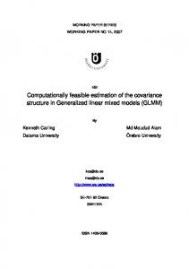
For selected values of n and m, we solved the linear program using GLPK (GNU Linear Programming Kit). In this subsection, we compare the resulting mechanisms with the Bailey-Cavallo mechanism. Worst-case performance In Table 2.1, we present the results for a single unit (m = 1). The second column displays the fraction of the total VCG payment that is not redistributed in the worst case by the worst-case optimal mechanism—that is, it displays the value 1 − k. (Displaying k would require too many significant digits.) Correspondingly, the third column displays the fraction of the total VCG payment that is not redistributed by the Bailey-Cavallo mechanism in the worst case (which is equal to n2 ). In Table 2.1, we showed that when m = 1, the worst-case optimal mechanism significantly outperforms the Bailey-Cavallo mechanism in the worst case. For larger m (m = 1, 2, 3, 4, n = m+2, . . . , 30), we compare the worst-case performance of these two mechanisms in Figure 2.1. We see that for any m, when n = m + 2, the worstcase optimal mechanism has the same worst-case performance as the Bailey-Cavallo mechanism (actually, in this case, the worst-case optimal mechanism is identical to 30

Table 2.1: Worst-case performances under the WCO and the Bailey-Cavallo mechanisms for single-item case. n Worst-Case Optimal Mechanism 3 66.7% 4 42.9% 5 26.7% 6 16.1% 7 9.52% 8 5.51% 9 3.14% 10 1.76% 15 8.55e-4 20 3.62e-5 30 5.40e-8 40 7.09e-11

Bailey-Cavallo Mechanism 66.7% 50.0% 40.0% 33.3% 28.6% 25.0% 22.2% 20.0% 13.3% 10.0% 6.67e-2 5.00e-2

the Bailey-Cavallo mechanism). When n > m+2, the worst-case optimal mechanism outperforms the Bailey-Cavallo mechanism (in the worst case). In Subsection 2.1.9, we will see that in the more general setting where agents have nonincreasing marginal values, the worst-case redistribution fraction for the (generalized) worst-case optimal mechanism is the same as for the unit demand setting. The same is true for the Bailey-Cavallo mechanism. Hence, Figure 2.1 does not change in this more general setting. Average-case performance It is perhaps not surprising that the worst-case optimal mechanism significantly outperforms the Bailey-Cavallo mechanism in the worst case, because that is, after all, the case for which the former has been designed. We can also compare how much the mechanisms redistribute on average (say, when the bids are drawn i.i.d. from a uniform distribution over [0, 1]). In this case, the worst-case optimal mechanism does not always outperform the Bailey-Cavallo mechanism. Table 2.2 compares the expected amount of VCG payment that fails to be redistributed by the worst-case 31

1

Worst−case Redistribution Fraction

0.9 0.8 0.7 0.6

1 Unit WO 1 Unit BC

0.5

2 Units WO 0.4

2 Units BC 3 Units WO

0.3

3 Units BC 4 Units WO

0.2

4 Units BC 0.1

5

10

15 20 Number of Agents

25

30

Figure 2.1: A comparison of the worst-case performance of the worst-case optimal mechanism (WCO) and the Bailey-Cavallo mechanism (BC).

optimal mechanism and by the Bailey-Cavallo mechanism (m = 1). We see that when n is small, the Bailey-Cavallo mechanism outperforms the worst-case optimal redistribution mechanism in expectation (except for the case n = 3, for which the two mechanisms are the same). When n is large (n ≥ 8), the worst-case optimal redistribution mechanism outperforms the Bailey-Cavallo mechanism. The results are similar for larger m. That is, when n is small, the BaileyCavallo mechanism outperforms the worst-case optimal redistribution mechanism in expectation (except for the case n = m + 2, for which the two mechanisms are the same). When n is large (e.g. n ≥ 10 for m = 2; n ≥ 13 for m = 3; n ≥ 16 for m = 4), the worst-case optimal redistribution mechanism performs better than the BaileyCavallo mechanism. In fact, this is not surprising: the expected amount that fails to be redistributed by the Bailey-Cavallo mechanism vanishes as Θ( n12 ). This is slower than the convergence rate of the worst-case redistribution fraction for the worst-case optimal mechanism (Corollary 1); and, of course, the average-case performance of 32

Table 2.2: Average-case performances under the WCO and the Bailey-Cavallo mechanisms for single-item case. n Worst-Case Optimal Mechanism 3 0.1667 4 0.1714 5 0.08889 6 0.06912 7 0.03571 8 0.02450 9 0.01255 10 0.008006 15 3.739e-4 20 1.726e-5 30 2.614e-8 40 3.461e-11

Bailey-Cavallo Mechanism 0.1667 0.1000 0.06667 0.04762 0.03571 0.02778 0.02222 0.01818 0.008333 0.004762 0.002151 0.001220

the worst-case optimal mechanism must be at least as good as its worst-case performance. This also shows that the worst-case optimal mechanism asymptotically outperforms the Bailey-Cavallo mechanism, even in the average case. A detailed example Finally, let us present the result for the case n = 5, m = 1 in detail. By solving the above linear program, we find that the optimal values for the ci are c2 = and c4 =

1 . 15

11 ,c 45 3

= − 19 ,

That is, the redistribution payment received by each agent under the

worst-case optimal mechanism is: agents, minus

1 9

11 45

times the second highest bid among the other

times the third highest bid among the other agents, plus

the fourth highest bid among the other agents. agent 1 receives

11 v 45 3

− 19 v4 +

1 v 15 5

agent 2 receives

11 v 45 3

− 19 v4 +

1 v 15 5

agent 3 receives

11 v 45 2

− 19 v4 +

1 v 15 5

agent 4 receives

11 v 45 2

− 19 v3 +

1 v 15 5

agent 5 receives

11 v 45 2

− 19 v3 +

1 v 15 4

33

1 15

times

The total amount redistributed by the worst-case optimal mechanism is 4 v 15 4

+

4 v; 15 5

in the worst case,

11 v 15 2

11 4 v + 15 v3 − 15 2

is redistributed. Hence, the fraction of the total

VCG payment that is not redistributed is never more than

4 15

= 26.7%.

As a specific example, for the bid vector v1 = 4, v2 = 3, v3 = 2, v4 = 1, v5 = 1, the total amount redistributed by the worst-case optimal redistribution mechanism is 4 4 4 11 v + 15 v3 − 15 v4 + 15 v5 15 2

=

11 4 4 4 3+ 15 2− 15 1+ 15 1 15

=

41 . 15

The total amount redistributed

by the Bailey-Cavallo mechanism is 25 v3 + 35 v2 = 52 2 + 35 3 =

13 . 5

Hence, for this bid

vector, the worst-case optimal redistribution mechanism redistributes more. As another specific example, for the bid vector v1 = 4, v2 = 3, v3 = 2, v4 = 2, v5 = 1, the total amount redistributed by the worst-case optimal redistribution mechanism is

11 v 15 2

+

4 v 15 3

−

4 v 15 4

+

4 v 15 5

=

11 3 15

+

4 2 15

−

4 2 15

+

amount redistributed by the Bailey-Cavallo mechanism is still

4 1 15

13 . 5

=

37 . 15

The total

Hence, for this bid

vector, the Bailey-Cavallo mechanism redistributes more. 2.1.6

Analytical Characterization

We recall that our linear program has the following form: Variables: cm+1 , cm+2 , . . . , cn−1 , k Maximize k (the fraction redistributed in the worst case) Subject to: Pj i=m+1 ci ≥ 0 for j = m + 1, . . . , n − 1 km ≤ (n − m − 1)cm+1 ≤ m P km ≤ n j=m+i−1 cj +(n−m−i)cm+i ≤ m for i = 2, . . . , n−m−1 j=m+1 Pj=n−1 km ≤ n j=m+1 cj ≤ m A linear program has no solution if and only if either the objective is unbounded, or the constraints are contradictory (there is no feasible solution). It is easy to see that k is bounded above by 1 (redistributing more than 100% violates the non-deficit constraint). Also, a feasible solution always exists, for example, k = 0 and ci = 0 for all i. So an optimal solution always exists. Observe that the linear program model 34

depends only on the number of agents n and the number of units m. Hence the optimal solution is a function of n and m. It turns out that this optimal solution can be analytically characterized as follows. Theorem 1. For any m and n with n ≥ m + 2, the worst-case optimal mechanism (among linear VCG redistribution mechanisms) is unique. For this mechanism, the fraction redistributed in the worst case is n−1 Pn−1m n−1
j=m j




∗

k =1−

The worst-case optimal mechanism is characterized by the following values for the ci : (−1)i+m−1 (n − m) c∗i = Pn−1 n−1
i j=m j

n−1 m−1




 n−1  X n−1

1 n−1 i


j=i

j

for i = m + 1, . . . , n − 1. It should be noted that we have proved ci = 0 for i ≤ m in Proposition 1. Proof. We first rewrite the linear program as follows. We introduce new variables P xm+1 , xm+2 , . . . , xn−1 , defined by xj = ji=m+1 ci for j = m + 1, . . . , n − 1. The linear program then becomes: Variables: xm+1 , xm+2 , . . . , xn−1 , k Maximize k Subject to: km ≤ (n − m − 1)xm+1 ≤ m km ≤ (m+i)xm+i−1 +(n−m−i)xm+i ≤ m for i = 2, . . . , n−m−1 km ≤ nxn−1 ≤ m xi ≥ 0 for i = m + 1, m + 2, . . . , n − 1 We will prove that for any optimal solution to this linear program, k = k ∗ . P Moreover, we will prove that when k = k ∗ , xj = ji=m+1 c∗i for j = m + 1, . . . , n − 1. This will prove the theorem. 35

We first make the following observations:

(n − m − 1)c∗m+1 n−1 Pn−1 (n−m)(m−1 ) 1 = (n − m − 1) (m+1) Pn−1 n−1 n−1 j=m+1 ( ) ( ) j=m m+1 j n−1 Pn−1 (n−m)(m−1 ) 1 = (n − m − 1) (m+1) Pn−1 n−1 ( n−1 j=m j=m ( j ) (m+1)

n−1 j

n−1 j







−

m(n−1) m = (n − m − 1) n−m−1 − (n − m − 1) (n−m−1) Pmn−1

j=m

n−1 m




)

(n−1 j )

= m − (1 − k ∗ )m = k ∗ m

For i = m + 1, . . . , n − 2, ic∗i + (n − i − 1)c∗i+1 =i

n−1 (−1)i+m−1 (n−m)(m−1 ) Pn−1 n−1 i j=m ( j )

+ (n − i − 1) =

(

− (n − i − 1) =

(

j

)

(

(

j=i

)




Pn−1

1 n−1 i+1

Pn−1

1 n−1 i

n−1 j

j=i

)

n−1 (−1)i+m (n−m)(m−1 ) Pn−1 n−1 (i+1) j=m ( j )

n−1 (−1)i+m−1 (n−m)(m−1 ) Pn−1 n−1 j=m

Pn−1

1 n−1 i

n−1 j=i+1 j

)




n−1 j




n−1 (−1)i+m−1 (n−m)(m−1 ) i+1 Pn−1 n−1 (i+1) j=m ( j ) (n−i−1) (n−1 ) i

Pn−1

j=i+1

n−1 (−1)i+m−1 (n−m)(m−1 ) Pn−1 n−1 j=m

(

j

)

= (−1)i+m−1 m(1 − k ∗ )

Finally, (n − 1)c∗n−1 = (n − 1)

n−1 (−1)n+m (n−m)(m−1 ) Pn−1 n−1 (n−1) j=m ( j )

Pn−1

1 n−1 n−1

(

)

n−1 j=n−1 j




= (−1)m+n m(1 − k ∗ )

36

n−1 j




Summarizing the above, we have: (n − m − 1)c∗m+1 = k ∗ m (m + 1)c∗m+1 + (n − m − 2)c∗m+2 = m(1 − k ∗ ) (m + 2)c∗m+2 + (n − m − 3)c∗m+3 = −m(1 − k ∗ ) (m + 3)c∗m+3 + (n − m − 4)c∗m+4 = m(1 − k ∗ ) .. . (n − 3)c∗n−3 + 2c∗n−2 = (−1)m+n−2 m(1 − k ∗ ) (n − 2)c∗n−2 + c∗n−1 = (−1)m+n−1 m(1 − k ∗ ) (n − 1)c∗n−1 = (−1)m+n m(1 − k ∗ )

Let x∗j =

Pj

∗ i=m+1 ci

for j = m + 1, m + 2, . . . , n − 1, the first equation in the

above tells us that (n − m − 1)x∗m+1 = k ∗ m. By adding the first two equations, we get (m + 2)x∗m+1 + (n − m − 2)x∗m+2 = m. By adding the first three equations, we get (m+3)x∗m+2 +(n−m−3)x∗m+3 = k ∗ m. By adding the first i equations, where i = 2, . . . , n−m−1, we get (m+i)x∗m+i−1 + (n − m − i)x∗m+i = m if i is even; (m + i)x∗m+i−1 + (n − m − i)x∗m+i = k ∗ m if i is odd. Finally by adding all the equations, we get nx∗n−1 = m if n − m is even; nx∗n−1 = k ∗ m if n − m is odd.

Thus, for all of the constraints other than the nonnegativity constraints, we have P shown that they are satisfied by setting xj = x∗j = ji=m+1 c∗i and k = k ∗ . We next show that the nonnegativity constraints are satisfied by these settings as well.

1 i+1

1 i

Pn−2

1 i+1

i!(n−1−i)! j=i j!(n−1−j)!

≥

1 i+1

Pn−2

(i+1)!(n−1−i−1)! j=i (j+1)!(n−1−j−1)!

=

n−1 j=i j n−1 i

Pn−1

For m + 1 ≤ i, i + 1 ≤ n − 1, we have

(

(

)

)

=

1 i

Pn−1

i!(n−1−i)! j=i j!(n−1−j)!

≥

(n−1 j ) ( )

Pn−1

j=i+1 n−1 i+1

This implies that the absolute value of c∗i is decreasing as i increases (if the c∗i

37

contains more than one number). We further observe that the sign of c∗i alternates, P with the first element c∗m+1 positive. So x∗j = ji=m+1 c∗i ≥ 0 for all j. Thus, we have shown that these xi = x∗i together with k = k ∗ form a feasible solution of the linear program. We proceed to show that it is in fact the unique optimal solution. First we prove the following proposition: ˆ xˆi , i = m + 1, m + 2, . . . , n − 1 satisfy the following inequalities: Proposition 4. If k, ˆ ≤ (n − m − 1)ˆ km xm+1 ≤ m ˆ ≤ (m + i)ˆ km xm+i−1 + (n − m − i)ˆ xm+i ≤ m for i = 2, . . . , n − m − 1 ˆ ≤ nˆ km xn−1 ≤ m kˆ ≥ k ∗ then we must have that xˆi = x∗i and kˆ = k ∗ . Proof of proposition. Consider the first inequality. We know that (n − m − ˆ ≥ k ∗ m = (n − m − 1)x∗ . It follows that xm+1 ≥ km 1)x∗m+1 = k ∗ m, so (n − m − 1)ˆ m+1 xˆm+1 ≥ x∗m+1 (n − m − 1 6= 0). Now, consider the next inequality for i = 2. We know that (m+2)x∗m+1 +(n−m− 2)x∗m+2 = m. It follows that (n−m−2)ˆ xm+2 ≤ m−(m+2)ˆ xm+1 ≤ m−(m+2)x∗m+1 = (n − m − 2)x∗m+2 , so xˆm+2 ≤ x∗m+2 (i = 2 ≤ n − m − 1 ⇒ n − m − 2 6= 0). Now consider the next inequality for i = 3. We know that (m + 3)x∗m+2 + (n − ˆ − (m + 3)ˆ m − 3)x∗m+3 = m. It follows that (n − m − 3)ˆ xm+3 ≥ km xm+2 ≥ k ∗ m − (m + 3)x∗m+2 = (n − m − 3)x∗m+3 , so xˆm+3 ≥ x∗m+3 (i = 3 ≤ n − m − 1 ⇒ n − m − 3 6= 0). Proceeding like this all the way up to i = n − m − 1, we get that xˆm+i ≥ x∗m+i if i is odd and xˆm+i ≤ x∗m+i if i is even. Moreover, if one inequality is strict, then all subsequent inequalities are strict. Now, if we can prove xˆn−1 = x∗n−1 , it would follow that the x∗i are equal to the xˆi (which also implies that kˆ = k ∗ ).

38

We consider two cases: Case 1: n − m is even. We have: n − m even ⇒ n − m − 1 odd ⇒ xˆn−1 ≥ x∗n−1 . We also have: n − m even ⇒ nx∗n−1 = m. Combining these two, we get m = nx∗n−1 ≤ nˆ xn−1 ≤ m ⇒ xˆn−1 = x∗n−1 . Case 2: n − m is odd. In this case, we have xˆn−1 ≤ x∗n−1 , and nx∗n−1 = k ∗ m. ˆ ≤ nˆ Then, we have: k ∗ m ≤ km xn−1 ≤ nx∗n−1 = k ∗ m ⇒ xˆn−1 = x∗n−1 . This completes the proof of the proposition. ˆ xˆi , i = m + 1, m + 2, . . . , n − 1 is a feasible solution and kˆ ≥ k ∗ , It follows that if k, then since all the inequalities in Proposition 4 are satisfied, we must have xˆi = x∗i and kˆ = k ∗ . Hence no other feasible solution is as good as the one described in the theorem. Knowing the analytical characterization of the worst-case optimal mechanism provides us with at least two major benefits. First, using these formulas is computationally more efficient than solving the linear program using a general-purpose solver. Second, we can derive the following corollary. Corollary 1. If the number of units m is fixed, then as the number of agents n increases, the worst-case fraction redistributed linearly converges to 1, with a rate of convergence 12 . (That is, limn→∞

∗ 1−kn+1 ∗ 1−kn

= 12 . That is, in the limit, the fraction that

is not redistributed halves for every additional agent.) We note that this is consistent with the experimental data for the single-unit case, where the worst-case remaining fraction roughly halves each time we add another agent. The worst-case fraction that is redistributed under the Bailey-Cavallo mechanism also converges to 1 as the number of agents goes to infinity, but the convergence is much slower—it does not converge linearly (that is, letting knC be the fraction redistributed by the Bailey-Cavallo mechanism in the worst case for n agents, 39

limn→∞

C 1−kn+1 C 1−kn

n = limn→∞ n+1 = 1). We now present the proof of the corollary.

Proof. When the number of agents is n, the worst-case fraction redistributed is kn∗ = (n−1 m ) ∗ n−1 . When the number of agents is n + 1, the fraction becomes kn+1 = ) ( j=m j

1−

Pn−1

1−

Pn

(mn ) For n sufficiently large, we will have 2n − mnm−1 > 0, and hence n . j=m ( j )

n−1 n−1 − m−1 n−1 (mn ) n−1 j=m ( j ) j=0 ( j ) n 2 P P = , and n n n−m 2n − m−1 (n) ( ) (n−1 ) j=m j=0 j m j
2n−1 n (because nj ≤ ni if j ≤ i). n−m 2n −mnm−1

∗ 1−kn+1 ∗ 1−kn

P

P

=

Since we have limn→∞ follows that limn→∞ 2.1.7

n 2n−1 −m(n−1)m−1 n−m 2n

∗ 1−kn+1 ∗ 1−kn

n 2n−1 −m(n−1)m−1 n−m 2n

= 12 , and limn→∞

≤

∗ 1−kn+1 ∗ 1−kn

2n−1 n n−m 2n −mnm−1

≤

= 12 , it

= 21 .

Worst-Case Optimality Outside the Family

In this subsection, we prove that the worst-case optimal redistribution mechanism among linear VCG redistribution mechanisms is in fact optimal (in the worst case) among all redistribution mechanisms that are deterministic, anonymous, strategyproof, efficient and satisfy the non-deficit constraint. Thus, restricting our attention to linear VCG redistribution mechanisms did not come at a loss. To prove this theorem, we need the following lemma. This lemma is not new: it was informally stated by Cavallo [20]. For completeness, we present it here with a detailed proof. Lemma 2. A VCG redistribution mechanism is deterministic, anonymous and strategyproof if and only if there exists a function f : Rn−1 → R, so that the redistribution payment zi received by i satisfies zi = f (v1 , v2 , . . . , vi−1 , vi+1 , . . . , vn ) for all i and all bid vectors. 40

Proof. First, let us prove the “only if” direction, that is, if a VCG redistribution mechanism is deterministic, anonymous and strategy-proof then there exists a deterministic function f : Rn−1 → R, which makes zi = f (v1 , v2 , . . . , vi−1 , vi+1 , . . . , vn ) for all i and all bid vectors. If a VCG redistribution mechanism is deterministic and anonymous, then for any bid vector v1 ≥ v2 ≥ . . . ≥ vn , the mechanism outputs a unique redistribution payment list: z1 , z2 , . . . , zn . Let G : Rn → Rn be the function that maps v1 , v2 , . . . , vn to z1 , z2 , . . . , zn for all bid vectors. Let H(i, x1 , x2 , . . . , xn ) be the ith element of G(x1 , x2 , . . . , xn ), so that zi = H(i, v1 , v2 , . . . , vn ) for all bid vectors and all 1 ≤ i ≤ n. Because the mechanism is anonymous, two agents should receive the same redistribution payment if their bids are the same. So, if vi = vj , H(i, v1 , v2 , . . . , vn ) = H(j, v1 , v2 , . . . , vn ). Hence, if we let j = min{t|vt = vi }, then H(i, v1 , v2 , . . . , vn ) = H(j, v1 , v2 , . . . , vn ). Let us define K : Rn → N × Rn as follows: K(y, x1 , x2 , . . . , xn−1 ) = [j, w1 , w2 , . . . , wn ], where w1 , w2 , . . . , wn are y, x1 , x2 , . . . , xn−1 sorted in descending order, and j = min{t|wt = y}. ({t|wt = y} = 6 ∅ because y ∈ {w1 , w2 , . . . , wn }). Also let us define F : Rn → R by F (vi , v1 , v2 , . . . , vi−1 , vi+1 , . . . , vn ) = H ◦ K(vi , v1 , v2 , . . . , vi−1 , vi+1 , . . . , vn ) = H(min{t|vt = vi }, v1 , v2 , . . . , vn ) = H(i, v1 , v2 , . . . , vn ) = zi . That is, F is the redistribution payment to an agent that bids vi when the other bids are v1 , v2 , . . . , vi−1 , vi+1 , . . . , vn . Since our mechanism is required to be strategy-proof, and the space of valuations is unrestricted, zi should be independent of vi by Lemma 1 in Cavallo [20]. Hence, we can simply ignore the first variable input to F ; let f (x1 , x2 , . . . , xn−1 ) = F (0, x1 , x2 , . . . , xn−1 ). So, we have zi = f (v1 , v2 , . . . , vi−1 , vi+1 , . . . , vn ) for all bid vectors and i. This completes the proof for the “only if” direction. For the “if” direction, if the redistribution payment received by i satisfies zi = f (v1 , v2 , . . . , vi−1 , vi+1 , . . . , vn ) for all bid vectors and i, then this is clearly a deter41

ministic and anonymous mechanism. To prove strategy-proofness, we observe that because an agent’s redistribution payment is not affected by her own bid, her incentives are the same as in the VCG mechanism, which is strategy-proof. Now we are ready to introduce the next theorem: Theorem 2. For any m and n with n ≥ m + 2, the worst-case optimal mechanism among the family of linear VCG redistribution mechanisms is worst-case optimal among all mechanisms that are deterministic, anonymous, strategy-proof, efficient and satisfy the non-deficit constraint. While we needed individual rationality earlier, this theorem does not mention it, that is, we cannot find a mechanism with better worst-case performance even if we sacrifice individual rationality. (The worst-case optimal linear VCG redistribution mechanism is of course individually rational.) Proof. Suppose there is a redistribution mechanism (when the number of units is m and the number of agents is n) that satisfies all of the above properties and has a better worst-case performance than the worst-case optimal linear VCG redistribution mechanism, that is, its worst-case redistribution fraction kˆ is strictly greater than k∗. By Lemma 2, for this mechanism, there is a function f : Rn−1 → R so that zi = f (v1 , v2 , . . . , vi−1 , vi+1 , . . . , vn ) for all i and all bid vectors. We first prove that f has the following properties. Proposition 5. f (1, 1, . . . , 1, 0, 0, . . . , 0) = 0 if the number of 1s is less than or equal to m. Proof of proposition. We assumed that for this mechanism, the worst-case redistribution fraction satisfies kˆ > k ∗ ≥ 0. If the total VCG payment is x, the total ˆ x] (non-deficit criterion). Consider the case redistribution payment should be in [kx, 42

where all agents bid 0, so that the total VCG payment is also 0. Hence, the total redistribution payment should be in [kˆ · 0, 0]—that is, it should be 0. Hence every agent’s redistribution payment f (0, 0, . . . , 0) must be 0. Now, let ti = f (1, 1, . . . , 1, 0, 0, . . . , 0) where the number of 1s equals i. We proved t0 = 0. If tn−1 = 0, consider the bid vector where everyone bids 1. The total VCG payment is m and the total redistribution payment is nf (1, 1, . . . , 1) = ntn−1 = 0. This corresponds to 0% redistribution, which is contrary to our assumption that kˆ > k ∗ ≥ 0. Now, consider j = min{i|ti 6= 0} (which is well-defined because tn−1 6= 0). If j > m, the property is satisfied. If j ≤ m, consider the bid vector where vi = 1 for i ≤ j and vi = 0 for all other i. Under this bid vector, the first j agents each get redistribution payment tj−1 = 0, and the remaining n − j agents each get tj . Thus, the total redistribution payment is (n − j)tj . Because the total VCG payment for this bid vector is 0, we must have (n − j)tj = 0. So tj = 0 (j ≤ m < n). But this is contrary to the definition of j. Hence f (1, 1, . . . , 1, 0, 0, . . . , 0) = 0 if the number of 1s is less than or equal to m. Proposition 6. f satisfies the following inequalities: ˆ ≤ (n − m − 1)tm+1 ≤ m km ˆ ≤ (m + i)tm+i−1 + (n − m − i)tm+i ≤ m for i = 2, 3, . . . , n − m − 1 km ˆ ≤ ntn−1 ≤ m km Here ti is defined as in the proof of Proposition 5. Proof of proposition. For j = m + 1, . . . , n, consider the bid vectors where vi = 1 for i ≤ j and vi = 0 for all other i. These bid vectors together with the nondeficit constraint and worst-case constraint produce the above set of inequalities: for example, when j = m + 1, we consider the bid vector vi = 1 for i ≤ m + 1 and vi = 0 for all other i. The first m + 1 agents each receive a redistribution payment of

43

tm = 0, and all other agents each receive tm+1 . Thus, the total VCG redistribution is (n − m − 1)tm+1 . The non-deficit constraint gives (n − m − 1)tm+1 ≤ m (because the ˆ total VCG payment is m). The worst-case constraint gives (n − m − 1)tm+1 ≥ km. Combining these two, we get the first inequality. The other inequalities can be obtained in the same way. We now observe that the inequalities in Proposition 6, together with kˆ ≥ k ∗ , are the same as those in Proposition 4 (where the ti are replaced by the xˆi ). Thus, we can conclude that kˆ = k ∗ , which is contrary to our assumption kˆ > k ∗ . Hence no mechanism satisfying all the listed properties has a redistribution fraction greater than k ∗ in the worst case. So far we have only talked about the case where n ≥ m + 2. For the purpose of completeness, we provide the following proposition for the n = m + 1 case. (We assume n > m in the unit demand setting.) Proposition 7. For any m and n with n = m+1, the original VCG mechanism (that is, redistributing nothing) is (uniquely) worst-case optimal among all redistribution mechanisms that are deterministic, anonymous, strategy-proof, efficient and satisfy the non-deficit constraint. We recall that when n = m + 1, Proposition 1 tells us that the only mechanism inside the family of linear redistribution mechanisms is the original VCG mechanism, so that this mechanism is automatically worst-case optimal inside this family. However, to prove the above proposition, we need to show that it is worst-case optimal among all redistribution mechanisms that have the desired properties. Proof. Suppose a redistribution mechanism exists that satisfies all of the above properties and has a worst-case performance as good as the original VCG mechanism, that

44

is, its worst-case redistribution fraction is greater than or equal to 0. This implies that the total redistribution payment of this mechanism is always nonnegative. By Lemma 2, for this mechanism, there is a function f : Rn−1 → R so that zi = f (v1 , v2 , . . . , vi−1 , vi+1 , . . . , vn ) for all i and all bid vectors. We will prove that f (x1 , x2 , . . . , xn−1 ) = 0 for all x1 ≥ x2 ≥ . . . ≥ xn−1 ≥ 0. First, consider the bid vector where vi = 0 for all i. Here, each agent receives a redistribution payment f (0, 0, . . . , 0). The total redistribution payment is then nf (0, 0, . . . , 0), which should be both greater than or equal to 0 (by the above observation) as well less than or equal to 0 (using the non-deficit criterion and the fact that the total VCG payment is 0). It follows that f (0, 0, . . . , 0) = 0. Now, let us consider the bid vector where v1 = x1 ≥ 0 and vi = 0 for all other i. For this bid vector, the agent with the highest bid receives a redistribution payment of f (0, 0, . . . , 0) = 0, and the other n − 1 agents each receive f (x1 , 0, . . . , 0). By the same reasoning as above, the total redistribution payment should be both greater than or equal to 0 and less than or equal to 0, hence f (x1 , 0, . . . , 0) = 0 for all x1 ≥ 0. Proceeding by induction, let us assume f (x1 , x2 , . . . , xk , 0, . . . , 0) = 0 for all x1 ≥ x2 ≥ . . . ≥ xk ≥ 0, for some k < n − 1. Consider the bid vector where vi = xi for i ≤ k + 1, and vi = 0 for all other i, where the xi are arbitrary numbers satisfying x1 ≥ x2 ≥ . . . ≥ xk ≥ xk+1 ≥ 0. For the agents with the highest k + 1 bids, their redistribution payment is specified by f acting on an input with only k non-zero variables. Hence they all receive 0 by induction assumption. The other n − k − 1 agents each receive f (x1 , x2 , . . . , xk , xk+1 , 0, . . . , 0). The total redistribution payment is then (n − k − 1)f (x1 , x2 , . . . , xk , xk+1 , 0, . . . , 0), which should be both greater than or equal to 0, and less than or equal to the total VCG payment. Now, in this bid vector, the lowest bid is 0 because k + 1 < n. But since n = m + 1, the total VCG payment is mvn = 0. So we have f (x1 , x2 , . . . , xk , xk+1 , 0, . . . , 0) = 0 for all x1 ≥ x2 ≥ . . . ≥ xk ≥ xk+1 ≥ 0. By induction, this statement holds for 45

all k < n − 1; when k + 1 = n − 1, we have f (x1 , x2 , . . . , xn−2 , xn−1 ) = 0 for all x1 ≥ x2 ≥ . . . ≥ xn−2 ≥ xn−1 ≥ 0. Hence, in this mechanism, the redistribution payment is always 0; that is, the mechanism is just the original VCG mechanism. Incidentally, we obtain the following corollary: Corollary 2. No VCG redistribution mechanism satisfies all of the following: determinism, anonymity, strategy-proofness, efficiency, and (strong) budget balance. This holds for any n ≥ m + 1. Proof. For the case n ≥ m + 2:

If such a mechanism exists, its worst-case perfor-

mance would be better than that of the worst-case optimal linear VCG redistribution mechanism, which by Theorem 1 obtains a redistribution fraction strictly less than 1. But Theorem 2 shows that it is impossible to outperform this mechanism in the worst case. For the case n = m + 1: If such a mechanism exists, it would perform as well as the original VCG mechanism in the worst case, which implies that it is identical to the VCG mechanism by Proposition 7. But the VCG mechanism is not (strongly) budget balanced. 2.1.8

Worst-Case Optimal Mechanism When Deficits Are Allowed

In the previous subsection, we showed that even if the individual rationality requirement is dropped, the worst-case optimal redistribution mechanism remains the same. In this subsection, we consider dropping the non-deficit requirement, and try to find the redistribution mechanism that deviates the least from budget balance (in the worst case). We define the imbalance to be the absolute difference between the total redistribution and the total VCG payment, and define the imbalance fraction to be the ratio between the imbalance and the total VCG payment. Our goal is to minimize the 46

worst-case imbalance fraction. Finding the optimal linear mechanism corresponds to the following optimization model: Minimize kd (the imbalance fraction in the worst case) Subject to: For every bid vector v1 ≥ v2 ≥ . . . ≥ vn ≥ 0 zn ≥ 0 (individual rationality) |z1 + z2 + . . . + zn − mvm+1 | ≤ kd mvm+1 (imbalance constraint) We recall that zi = c0 + c1 v1 + c2 v2 + . . . + ci−1 vi−1 + ci vi+1 + . . . + cn−1 vn The imbalance constraint can also be written as (1 − kd )mvm+1 ≤ z1 + z2 + . . . + zn ≤ (1 + kd )mvm+1 The above optimization model can be transformed into a linear program, based on the following observations. Proposition 8. If c0 , c1 , . . . , cn−1 satisfy both the individual rationality and the imbalance constraints, then ci = 0 for i = 0, . . . , m. The proof is a slight modification of the proof of Proposition 1. Proof. First, let us prove that c0 = 0. Consider the bid vector in which vi = 0 for all i. To obtain individual rationality, we must have c0 ≥ 0. To satisfy the imbalance constraint, we must have c0 ≤ 0. Thus we know c0 = 0. Now, if ci = 0 for all i, there is nothing to prove. Otherwise, let j = min{i|ci 6= 0}. Assume that j ≤ m. We recall that we can write the individual rationality constraint as follows: zn = c0 + c1 v1 + c2 v2 + c3 v3 + . . . + cn−2 vn−2 + cn−1 vn−1 ≥ 0 for any bid vector. Let us consider the bid vector in which vi = 1 for i ≤ j and vi = 0 for the rest. In this case zn = cj , so we must have cj ≥ 0. The imbalance constraint requires that : z1 + z2 + . . . + zn ≤ (1 + kd )mvm+1 for any bid vector. Consider the same bid vector as above. We have zi = 0 for i ≤ j, because for these bids, the jth highest other bid has value 0, so all the ci that are nonzero are multiplied by 0. For i > j, we have zi = cj , because the jth highest other bid has value 1, and all lower bids have value 47

0. So the imbalance constraint tells us that cj (n − j) ≤ (1 + kd )mvm+1 . Because j ≤ m, vm+1 = 0, so the right hand side is 0. We also have n − j > 0 because j ≤ m < n. So cj ≤ 0. Because we have already established that cj ≥ 0, it follows that cj = 0; but this is contrary to assumption. So j > m. Proposition 9. The imbalance constraint can be written as linear inequalities involving only the ci and kd . The proof is a slight modification of the proof of Proposition 3. Proof. The imbalance constraint requires that for any bid vector, (1 − kd )mvm+1 ≤ z1 + z2 + . . . + zn ≤ (1 + kd )mvm+1 , where zi = c0 + c1 v1 + c2 v2 + . . . + ci−1 vi−1 + ci vi+1 + . . . + cn−1 vn for i = 1, 2, . . . , n. Because ci = 0 for i ≤ m, we can simplify this inequality to qm+1 vm+1 + qm+2 vm+2 + . . . + qn vn ≥ 0 qm+1 = (n − m − 1)cm+1 − (1 − kd )m qi = (i − 1)ci−1 + (n − i)ci , for i = m + 2, . . . , n − 1 qn = (n − 1)cn−1

Qm+1 vm+1 + Qm+2 vm+2 + . . . + Qn vn ≤ 0 Qm+1 = (n − m − 1)cm+1 − (1 + kd )m Qi = (i − 1)ci−1 + (n − i)ci , for i = m + 2, . . . , n − 1 Qn = (n − 1)cn−1

By Lemma 1, this is equivalent to Pj

i=m+1

Pj

i=m+1 qi

≥ 0 for j = m + 1, . . . , n and

Qi ≤ 0 for j = m + 1, . . . , n. So, we can simplify further as follows:

(1 − kd )m ≤ (n − m − 1)cm+1 ≤ (1 + kd )m P (1 − kd )m ≤ n j=m+i−1 cj + (n − m − i)cm+i ≤ (1 + kd )m for i = 2, . . . , n − m − 1 j=m+1 48

(1 − kd )m ≤ n

Pj=n−1

j=m+1 cj

≤ (1 + kd )m

So, the imbalance constraint can also be written as a set of linear inequalities involving only the ci and kd . Combining all the propositions (together with Proposition 2), we see that the original optimization problem can be transformed into the following linear program. Variables: cm+1 , cm+2 , . . . , cn−1 , kd Minimize kd (the imbalance fraction in the worst case) Subject to: Pj i=m+1 ci ≥ 0 for j = m + 1, . . . , n − 1 (1 − kd )m ≤ (n − m − 1)cm+1 ≤ (1 + kd )m Pj=m+i−1 cj + (n − m − i)cm+i ≤ (1 + kd )m for (1 − kd )m ≤ n j=m+1 i = 2, . . . , n − m P− 1 (1 − kd )m ≤ n j=n−1 j=m+1 cj ≤ (1 + kd )m For this model, it is easy to see that kd is bounded below by 0. Also, kd = 1 and ci = 0 for all i form a feasible solution. So an optimal solution always exists. As in the case where deficits are not allowed, the optimal solution can be analytically characterized. The characterization is the following: Theorem 3. For any m and n with n ≥ m + 2, the worst-case optimal mechanism with deficits (among linear VCG redistribution mechanisms) is unique. For this mechanism, the imbalance fraction in the worst case is n−1 m




kd∗

= Pn

n j=m+1 j




The worst-case optimal mechanism with deficits is characterized by the following values for the ci : 2(−1)i+m−1 (n − m)
P c∗i = i nj=m+1 nj

n−1 m−1

49




 n−1  X n−1

1 n−1 i


j=i

j

for i = m + 1, . . . , n − 1. From Proposition 8 it follows that ci = 0 for i ≤ m. Proof. Let α = kd∗ /(1−k ∗ ), where k ∗ is the worst-case optimal redistribution fraction in Theorem 1. To avoid ambiguity, we refer to the c∗i in Theorem 1 as cw∗ i , and to d∗ w∗ the c∗i here as cd∗ for all i. We have shown in i . Inspection reveals that ci = 2αci

Theorem 1 that Pj w∗ i=m+1 ci ≥ 0 for j = m + 1, . . . , n − 1 k ∗ m ≤ (n − m − 1)cw∗ m+1 ≤ m P w∗ cw∗ k ∗ m ≤ n j=m+i−1 j + (n − m − i)cm+i ≤ m for i = 2, . . . , n − m − 1 j=m+1 P w∗ k ∗ m ≤ n j=n−1 j=m+1 cj ≤ m

So we have Pj d∗ i=m+1 ci ≥ 0 for j = m + 1, . . . , n − 1 (α is positive) 2αk ∗ m ≤ (n − m − 1)cd∗ m+1 ≤ 2αm P d∗ cd∗ 2αk ∗ m ≤ n j=m+i−1 j + (n − m − i)cm+i ≤ 2αm for i = 2, . . . , n − m − 1 j=m+1 P d∗ 2αk ∗ m ≤ n j=n−1 j=m+1 cj ≤ 2αm

A sequence of algebraic manipulations reveals that 2αk ∗ = (1 − kd∗ ) and 2α = (1 + kd∗ ). Hence, kd∗ and the cd∗ i form a feasible solution, because we have Pj d∗ i=m+1 ci ≥ 0 for j = m + 1, . . . , n − 1 ∗ (1 − kd∗ )m ≤ (n − m − 1)cd∗ m+1 ≤ (1 + kd )m P d∗ ∗ (1 − kd∗ )m ≤ n j=m+i−1 cd∗ j + (n − m − i)cm+i ≤ (1 + kd )m for i = 2, . . . , n − m − 1 j=m+1 Pj=n−1 d∗ (1 − kd∗ )m ≤ n j=m+1 cj ≤ (1 + kd∗ )m

We proceed to show that it is in fact the unique optimal solution. Suppose cˆi and kˆd form a feasible solution, and kˆd ≤ kd∗ . We have 50

(1 − kd∗ )m ≤ (1 − kˆd )m ≤ (n − m − 1)ˆ cm+1 ≤ (1 + kˆd )m ≤ (1 + kd∗ )m P (1−kd∗ )m ≤ (1− kˆd )m ≤ n j=m+i−1 cˆj +(n−m−i)ˆ cm+i ≤ (1+ kˆd )m ≤ (1+kd∗ )m j=m+1 for i = 2, . . . , n − m − 1 P (1 − kd∗ )m ≤ (1 − kˆd )m ≤ n j=n−1 ˆj ≤ (1 + kˆd )m ≤ (1 + kd∗ )m j=m+1 c

We introduce new variables xm+1 , xm+2 , . . . , xn−1 , defined by xj =

1 2α

Pj

ˆi i=m+1 c

for j = m + 1, . . . , n − 1. The above inequalities can be rewritten in terms of xi , we have k ∗ m ≤ (n − m − 1)xm+1 ≤ m k ∗ m ≤ (m + i)xm+i−1 + (n − m − i)xm+i ≤ m for i = 2, . . . , n − m − 1 k ∗ m ≤ nxn−1 ≤ m

However, in Proposition 4, we proved that these inequalities have a unique solution. Therefore, there is only one value that each of cˆi and kˆd can have. This proves that kd∗ and the cd∗ i form the unique optimal solution. α = kd∗ /(1 − k ∗ ) can be interpreted as the ratio between the imbalance fraction of the worst-case optimal mechanism with deficits (among linear VCG redistribution mechanisms) and the imbalance fraction of the worst-case optimal mechanism without deficits. This ratio can be expressed as follows: α=

kd∗ /(1

∗

−k )=

n−1 j=m j Pn n j=m+1 j

Pn−1

(

) = ()

n−1 j=m+1 j−1 Pn n j=m+1 j

Pn

(

()

)

n j=m+1 ((j/n) j Pn n j=m+1 j

Pn

=

( )) ()

For fixed n, this ratio increases as m increases. (This is because as we decrease m by 1, the ratio of the additional terms in the fraction decreases.) When m = 1, α =

2n−1 −1 2n −n−1

(for large n, roughly

1 ); 2

when m = n − 2, α =

n n+1

(for large n,

roughly 1). Hence, if m is small (relative to n), the worst-case optimal linear VCG redistribution mechanism with deficits is much closer to budget balance than the worst-case optimal mechanism without deficits; if m is large (relative to n), they are 51

1 0.8 n=10

0.6 0

2

4

6

8

10

1 0.8 n=20

0.6 0

5

10

15

20

1 0.8 n=30

0.6 0

5

10

15

20

25

30

1 0.8 n=40

0.6 0

10

20

30

40

Figure 2.2: The ratio between the imbalance fractions of the worst-case optimal mechanisms with and without deficits. about the same. On the other hand, when m is small relative to n, then the worstcase optimal redistribution fraction is large even with the non-deficit requirement. This means that the non-deficit constraint does not come at a great cost. Figure 2.2 shows how α changes as a function of m and n. Now we prove that the worst-case optimal linear VCG redistribution mechanism with deficits is in fact optimal among all redistribution mechanisms that are deterministic, anonymous, strategy-proof and efficient. Theorem 4. For any m and n with n ≥ m + 2, the worst-case optimal mechanism with deficits among linear VCG redistribution mechanisms has the smallest worst-case imbalance fraction among all VCG redistribution mechanisms that are deterministic, anonymous, strategy-proof and efficient. As in the case of Theorem 2, there is no redistribution mechanism with a smaller worst-case imbalance fraction even if we sacrifice individual rationality. 52

Proof. Suppose there is a redistribution mechanism (when the number of units is m and the number of agents is n) that satisfies all of the above properties and has a smaller worst-case imbalance fraction than that of the worst-case optimal linear VCG redistribution mechanism with deficits—that is, its worst-case imbalance fraction kˆd is strictly less than kd∗ . By Lemma 2, for this mechanism, there is a function f : Rn−1 → R so that zi = f (v1 , v2 , . . . , vi−1 , vi+1 , . . . , vn ) for all i and all bid vectors. The following properties of f follow from straightforward modifications of the proofs of Proposition 5 and Proposition 6. Proposition 10. f (1, 1, . . . , 1, 0, 0, . . . , 0) = 0 if the number of 1s is less than or equal to m. Proposition 11. f satisfies the following inequalities: (1 − kˆd )m ≤ (n − m − 1)tm+1 ≤ (1 + kˆd )m (1 − kˆd )m ≤ (m + i)tm+i−1 + (n − m − i)tm+i ≤ (1 + kˆd )m for i = 2, 3, . . . , n − m − 1 (1 − kˆd )m ≤ ntn−1 ≤ (1 + kˆd )m ti = f (1, 1, . . . , 1, 0, 0, . . . , 0) where the number of 1s equals i Let xi =

1 t 2α i

for i = m + 1, . . . , n − 1. Since kˆd < kd∗ , we have

k∗m
m.8 (Otherwise, it is clearly optimal to give every agent a unit and charge nothing.) As usual, for the ith agent, we denote her true/reported type/bid for winning one unit by vi (we are focusing on strategy-proof mechanisms). Without losing generality, we assume that v1 ≥ v2 ≥ . . . ≥ vn ≥ 0. Let constants L and U be the lower and upper bounds, respectively, on the possible values. Hence, ∞ > U ≥ v1 ≥ v2 ≥ . . . ≥ vn ≥ L ≥ 0. We assume that we have a prior joint probability distribution over the agents’ values vi . We denote the probability density function of this joint distribution by f (v1 , . . . , vn ). We emphasize that we require neither that the agents’ values are drawn from identical distributions, nor that they are independent. We aim to design VCG redistribution mechanisms that redistribute the most in expectation, subject to the non-deficit constraint. Here, we do not explicitly enforce the individual rationality constraint for the following reasons: Since our objective is to maximize social welfare, if the prior distribution is symmetric across agents, then under any redistribution mechanism that redistributes a nonnegative amount of payment in expectation, every agent benefits from participating in the mechanism (the agent receives nonnegative expected utility). That is, ex-interim individual rationality is not a binding constraint. Our technique can also be used to design mechanisms that are ex-interim individually rational when the prior is not symmetric across agents, or mechanisms that satisfy the even stronger ex-post individual rationality. However, this would require additional constraints and make the ana8

We remove this restriction in Subsection 2.2.5 where we consider settings without unit demand.

67

lytical characterization in Subsection 2.2.2 too complex. For the above reasons, we omit individual rationality constraints. 2.2.2

Linear Redistribution Mechanisms

We first restrict our attention to the family of linear redistribution mechanisms. We recall from Subsection 2.1.2 that a linear redistribution mechanism is characterized by a linear redistribution function of the following form: r(v−i ) = c0 + c1 v−i,1 + c2 v−i,2 + . . . + cn−1 v−i,n−1 Here, r(v−i ) is agent i’s redistribution. v−i,j is the jth highest bid among v−i (the set of bids other than vi ). The coefficients cj completely characterize the redistribution mechanism. Optimal-in-expectation linear redistribution mechanisms We will prove the following result, which characterizes a linear redistribution mechanism that maximizes the expected total redistribution (among linear redistribution mechanisms). We call this mechanism OEL (optimal-in-expectation, linear). Theorem 6. Given n, m, and a prior distribution over agents’ valuations, the following ci define a redistribution mechanism that maximizes expected redistribution, under the constraints that the mechanism must be a linear redistribution mechanism, efficient, strategy-proof, and satisfy the non-deficit property. Let the oi be defined as follows: o0 = U − Ev1 , oi = Evi − Evi+1 (i = 1, 2, . . . , n − 1), and on = Evn − L. The oi are determined by the given prior distribution. Let k be any integer satisfying k ∈ arg mini {oi /

n i


|i − m odd, i = 0, . . . , n} 68

Let function G be defined as follows: G(n, m, i) =

n−i−1 n−m−1


/

m−1 i−1




=

(n−i−1)!(i−1)! (n−m−1)!(m−1)!

• If 0 < k < m, then ci = (−1)m−i G(n, m, i) for i = k + 1, . . . , m, ck = m/n −

Pm

m−i G(n, m, i), i=k+1 (−1)

and ci = 0 for other i. • If k = 0, then ci = (−1)m−i G(n, m, i) for i = 1, . . . , m, c0 = U m/n − U

Pm

m−i G(n, m, i), i=1 (−1)

and ci = 0 for other i. • If m < k < n, then ci = (−1)m−i−1 G(n, m, i) for i = m + 1, . . . , k − 1, ck = m/n −

Pk−1

m−i−1 G(n, m, i), i=m+1 (−1)

and ci = 0 for other i. • If k = n, then ci = (−1)m−i−1 G(n, m, i) for i = m + 1, . . . , n − 1, c0 = Lm/n − L

Pn−1

m−i−1 G(n, m, i), i=m+1 (−1)

and ci = 0 for other i. In expectation, this mechanism fails to redistribute ok m

n−1 m




69

/

n k




This mechanism is uniquely optimal among all linear redistribution mechanisms if and only if the choice of k is unique and there does not exist an even i and an odd j such that oi = oj = 0. The mechanism is complicated, and is perhaps easier to understand using the auxiliary variables that we define in the derivation of this mechanism below. Depending on the optimal choice of k, we have different OEL mechanisms. We call the OEL mechanism corresponding to a specific choice of k the OEL mechanism with index k. For k = 1, 2, . . . , n−1, the waste under the OEL mechanism with index
n
k equals m n−1 / k (vk − vk+1 ). The waste under the OEL mechanism with index 0 m
equals m n−1 (U − v1 ). The waste under the OEL mechanism with index n equals m
m n−1 (vn −L). Basically, the waste is always a multiple of: 1) the expected difference m between two adjacent (in terms of size) bids, or 2) the expected difference between the upper bound and the largest bid, or 3) the expected difference between the lowest bid and the lower bound. Moreover, the multiplication coefficient is determined by m and n. Then, the OEL mechanism simply chooses the best of these options. In contrast, under the worst-case optimal mechanism, the waste is a linear combination of all of the bids (except for the highest m). In what follows, we derive the OEL mechanism and prove its optimality. Our objective is to find an linear redistribution mechanism that redistributes the most in expectation. To optimize among the family of linear redistribution mechanisms, we must solve for the optimal values of the ci . We want the resulting redistribution mechanism to be strategy-proof and efficient, and we want it to satisfy the nondeficit property. The first two properties are satisfied by all the mechanisms inside the linear family, so the only constraint is the non-deficit property. The following optimization model can be used to find the linear redistribution mechanism (the ci ) that redistributes the most in expectation, while satisfying the non-deficit property. 70

Variables: c0 ,P c1 , . . . , cn−1 Maximize E( ni=1 ri ) Subject to: For every bid vector U ≥ v1 ≥ v2 ≥ . . . ≥ vn ≥ L P n i=1 ri ≤ mvm+1 ri = c0 + c1 v−i,1 + c2 v−i,2 + . . . + cn−1 v−i,n−1 Given the prior distribution, E(mvm+1 ) is a constant, so the objective of the P above model may be rewritten as Minimize E(mvm+1 − ni=1 ri ). Since ri = c0 + c1 v−i,1 + c2 v−i,2 + . . . + cn−1 v−i,n−1 , where v−i,j is the jth highest bid among bids other than i’s own bid, we have the following: r1 = c0 + c1 v2 + c2 v3 + c3 v4 . . . + cn−2 vn−1 + cn−1 vn r2 = c0 + c1 v1 + c2 v3 + c3 v4 . . . + cn−2 vn−1 + cn−1 vn r3 = c0 + c1 v1 + c2 v2 + c3 v4 . . . + cn−2 vn−1 + cn−1 vn ... rn−1 = c0 + c1 v1 + c2 v2 + c3 v3 . . . + cn−2 vn−2 + cn−1 vn rn = c0 + c1 v1 + c2 v2 + c3 v3 . . . + cn−2 vn−2 + cn−1 vn−1 We can write mvm+1 −

Pn

i=1 ri

as q0 +q1 v1 +q2 v2 +. . .+qn vn , where the coefficients

qi are listed below: q0 = −nc0 qi = −(i − 1)ci−1 − (n − i)ci for i = 1, 2, . . . , m, m + 2, . . . , n qm+1 = m − mcm − (n − m − 1)cm+1 (We note that we introduced a dummy variable cn in the above equations—since there are only n − 1 other bids, cn will always be multiplied by 0, but adding this variable makes the definition of the qi more elegant.) Given n and m, q0 , . . . , qn (n + 1 values) are determined by c0 , . . . , cn−1 (n values). Conversely, if q0 , . . . , qn−1 are fixed, then we can completely solve for the values of c0 , . . . , cn−1 (and hence also for qn ). This results in the following relation among the qi : 71

q1 −

n−1 q 1! 2

+

(n−1)(n−2) q3 2!

−

(n−1)(n−2)(n−3) q4 3!

+ . . . + (−1)n−1 (n−1)(n−2)...2·1 qn = (n−1)!

(−1)m m (n−1)(n−2)...(n−m) m! After simplification we obtain: Pn

i=1 (−1)

i−1 n−1 i−1




qi = (−1)m m

n−1 m




Now, we can use the qi as the variables of the optimization model, since from them P we will be able to infer the ci . Because mvm+1 − ni=1 ri = q0 +q1 v1 +q2 v2 +. . .+qn vn , we can rewrite the non-deficit constraint by requiring that the latter summation is nonnegative. Also, the qi must satisfy the previous inequality (otherwise there will be no corresponding ci ). Variables: q0 , q1 , . . . , qn Minimize E(q0 + q1 v1 + q2 v2 + . . . + qn vn ) Subject to: For every bid vector U ≥ v1 ≥ v2 ≥ . . . ≥ vn ≥ L qP 0 + q1 v1 + q2 v2 +
. . . + qn vnm≥ 0n−1
n i−1 n−1 (−1) q = (−1) m m i=1 i−1 i In what follows, we will cast the above model into a linear program. We begin with the following lemma: Lemma 3. The following are equivalent: (1) q0 + q1 v1 + q2 v2 + . . . + qn vn ≥ 0 for all U ≥ v1 ≥ v2 ≥ . . . ≥ vn ≥ L P P (2) q0 + L ni=1 qi + (U − L) ki=1 qi ≥ 0 for k = 0, . . . , n Proof. (1)⇒(2): (2) can be obtained from (1) by setting v1 = v2 = . . . = vk = U and vk+1 = vk+2 = . . . = vn = L. P (2)⇒(1): Let us rewrite T = q0 + q1 v1 + q2 v2 + . . . + qn vn as q0 + L ni=1 qi + P P P Pn (v1 − v2 ) 1i=1 qi + (v2 − v3 ) 2i=1 qi + . . . + (vn−1 − vn ) n−1 i=1 qi + (vn − L) i=1 qi . If Pk Pn i=1 qi ≥ 0 for every k = 1, . . . , n, then T ≥ q0 + L i=1 qi ≥ 0 (because v1 − v2 , v2 − 72

v3 , . . . , vn − L are all nonnegative). Otherwise, let k 0 be the index so that

Pk 0

i=1 qi

is minimal (hence negative). To make T minimal, we want vk0 − vk0 +1 (which is P0 P multiplied by ki=1 qi ) to be maximal. So the minimal value for T is q0 + L ni=1 qi + P0 (U − L) ki=1 qi ≥ 0, which is attained when v1 = v2 = . . . = vk0 = U and vk0 +1 = vk0 +2 = . . . = vn = L. Hence T is always nonnegative. Let xk = (q0 + L

Pn

i=1 qi )/(U

− L) +

Pk

i=1 qi

for k = 0, . . . , n. The xi correspond

(one to one) to the qi , so we can use the xi as the variables in the optimization model. The first constraint of the optimization model now becomes xk ≥ 0 for every k. Since xk − xk−1 = qk for k = 1, . . . , n, the second constraint becomes Pn

i−1 n−1 i=1 (−1) i−1


(xi − xi−1 ) = (−1)m m

n−1 m




After simplification we get: Pn

i i=0 (−1)

n i


xi = (−1)m−1 m

n−1 m




Let o0 = U − Ev1 , oi = Evi − Evi+1 (i = 1, . . . , n − 1) and on = Evn − L. The oi are all nonnegative constants that we know from the prior distribution. The objective of the optimization model can be rewritten as follows: E(q0 + q1 v1 + q2 v2 + . . . + qn vn ) = q0 + q1 Ev1 + q2 Ev2 + . . . + qn Evn = x0 (U − L) + q1 (Ev1 − L) + q2 (Ev2 − L) + . . . + qn (Evn − L) = x0 ((U − L) − (Ev1 − L)) + (x0 + q1 )((Ev1 − L) − (Ev2 − L)) + (x0 + q1 + q2 )((Ev2 − L) − (Ev3 − L)) + . . . + (x0 + q1 + . . . + qn )(Evn − L) = o0 x0 + o1 x1 + . . . + on xn We finally obtain the following linear program:

73

Variables: x0 , x1 , . . . , xn Minimize o0 x0 + o1 x1 + . . . + on xn Subject to: xi ≥ 0

P n i n m−1 m n−1 i=0 (−1) i xi = (−1) m At this point, for any given n and m, for any prior distribution, it is possible to solve this linear program using any LP solver; then, using the above, the resulting xi can be transformed back to ci to obtain an optimal-in-expectation linear redistribution mechanism. However, this will not be necessary. The following proposition gives an analytical solution of this linear program. Proposition 20. Let k be any integer satisfying k ∈ arg mini {oi /

n i


|i − m odd, i = 0, . . . , n}

The above linear program has the following optimal solution: xk = m

n−1 m


n
/ k , and xi = 0 for i 6= k

The optimal objective value is ok m

n−1 m




/

n k




This solution is the unique optimal solution if and only if the choice of k is unique and there does not exist an even i and an odd j such that oi = oj = 0. Proof. We can rewrite the second constraint as Pn

n i




i−m+1 i=0 ((−1)

n−1 m




)/(m

)xi = 1

This results in the program Variables: x0 , x1 , . . . , xn Minimize o0 x0 + o1 x1 + . . . + on xn Subject to: xi ≥ P 0

P n n−1 /(m )xi = i m i=0...n;i−m odd

i=0...n;i−m even

74

n i


/(m

n−1 m




)xi + 1

The oi are nonnegative. To minimize the objective, we want all the xi to be as small as possible. It is not hard to see that it does not hurt to set the xi for which i − m is even to zero: in fact, setting them to a larger value will only force the xi for which i − m is odd to take on larger values, by the last constraint. (It should be noted that if there exists an even i and an odd j such that oi = oj = 0, then we can increase the corresponding xi and xj at no cost to the objective without breaking the constraint, hence the solution is not unique in that case.) This results in the following linear program: Variables: x0 , x1 , . . . , xn Minimize o0 x0 + o1 x1 + . . . + on xn Subject to: xi ≥ P 0

n n−1 /(m )xi = 1 i m i=0...n;i−m odd

We want the xi to be as small as possible. However, the second constraint makes it impossible to set all the xi to 0. For each xi with i − m odd, if we increase it by δ,

the left side of the second constraint is increased by ni /(m n−1 )δ and the objective m value is increased by oi δ. We need the left side of the second constraint to increase to 1 (starting from 0), while minimizing the increase in the objective value. To do so, we want to find the xi (with i − m odd) that has the minimal cost-gain ratio

(where the cost is oi δ, and the gain is ni /(m n−1 )δ). It follows that for any integer m
k satisfying k ∈ arg mini {oi / ni |i − m odd, i = 0, . . . , n}, the linear program has the
n
following optimal solution: xk = m n−1 / k and xi = 0 for i 6= k. The resulting m

/ nk . optimal objective value is ok m n−1 m In the above argument, there were only two conditions under which we made a choice that is not necessarily uniquely optimal: if (and only if) there exists an even i and an odd j such that oi = oj = 0, then, as we explained, there exist optimal solutions where some xi with m−i even is set to a positive value (in fact, it can be set 75

to any value in this case); and if (and only if) arg mini {oi /

n i




|i−m odd, i = 0, . . . , n}

is not a singleton set, then there exists another optimal solution with another xk set to a positive value (in fact, in this case, multiple xk may simultaneously be set to a positive value). By transforming the xi from Proposition 20 to the corresponding ci , we obtain the OEL mechanism from Theorem 6. We now present a special case that may give some further intuition. The case where k = m + 1 in Theorem 6 corresponds to the redistribution mechanism in which each agent receives a redistribution payment that is equal to m/n times the (m+1)th highest bid from the other agents. In our setting of multi-unit auctions with unit demand, this is exactly the Bailey-Cavallo mechanism. This observation is formally stated in the following corollary. Corollary 3. Given n, m, and a prior distribution over agents’ valuations, we define the oi as follows: o0 = U − Ev1 , oi = Evi − Evi+1 (i = 1, 2, . . . , n − 1), and on = Evn − L. If the following condition holds: om+1 ≤ oi

n m+1




/

n i




for all 0 ≤ i ≤ n with i − m odd,

then the Bailey-Cavallo mechanism maximizes expected redistribution, under the constraints that the mechanism must be a linear redistribution mechanism, efficient, strategy-proof, and satisfy the non-deficit property. Next, we present two example OEL mechanisms. Example 3. Consider the case where n = 3 and m = 1, and the bids are all drawn independently and uniformly from [0, 1]. In this case, Evi = So, U = 1, L = 0, oi =

1 4

4−i 4

for i = 1, . . . , 3.

for i = 0, . . . , 3. (We recall that o0 = U − Ev1 , on = 76

Evn − L, and oi = Evi − Evi+1 otherwise.) arg mini {oi /

n i


|i − m odd, i = 0, . . . , n}

is then {m + 1} = {2}. The expected amount that fails to be redistributed is
n
o2 m n−1 / 2 = 61 . (The expected total VCG payment is 12 .) The optimal solution m is given by c2 = 31 , and ci = 0 for other i. Hence, this optimal-in-expectation linear redistribution mechanism is defined by ri =

1 v , 3 −i,2

Cavallo mechanism. The total redistribution is

Pn

which is actually the Bailey-

i=1 ri

= 13 v2 + 23 v3 . The expected

amount that fails to be redistributed is E(v2 − 31 v2 − 23 v3 ) = 23 E(v2 − v3 ) = 61 . Example 4. Consider the case where n = 8 and m = 2, and the bids are all drawn for i = 1, . . . , 8. So independently and uniformly from [0, 1]. In this case, Evi = 9−i 9
U = 1, L = 0, oi = 19 for i = 0, . . . , 8. arg mini {oi / ni |i − m odd, i = 0, . . . , n} is then
n
1 . {3, 5}. The expected amount that fails to be redistributed is o3 m n−1 / 3 = 12 m (The expected total VCG payment is 43 .) One optimal solution is given by c3 =

1 , 4

and ci = 0 for other i. Hence this

expectation optimal linear redistribution mechanism is defined by ri = 14 v−i,3 (BaileyP Cavallo mechanism). The total redistribution is ni=1 ri = 45 v3 + 34 v4 . The expected amount that fails to be redistributed is E(2v3 − 54 v3 − 34 v4 ) = 43 E(v3 − v4 ) = 3 The other optimal solution is given by c3 = 25 , c4 = − 10 , c5 =

3 , 20

1 . 12

and ci = 0 for

other i. Hence this expectation optimal linear redistribution mechanism is defined P 3 3 by ri = 25 v−i,3 − 10 v−i,4 + 20 v−i,5 . The total redistribution is ni=1 ri = 2v3 − 34 v5 + 34 v6 . The expected amount that fails to be redistributed is E( 43 (v5 − v6 )) =

1 . 12

Properties of the OEL mechanism We present some properties of the OEL mechanism. First, we have that there cannot be another redistribution mechanism that always redistributes at least as much in total as OEL, and strictly more in at least one case. That is, the OEL mechanism is collectively undominated.

77

Proposition 21. For any m, n and any prior distribution, there does not exist any redistribution mechanism that, for every multi-set of bids, redistributes at least as much in total as OEL, and redistributes strictly more in at least one case. We will prove the above proposition in Section 2.3. More precisely, we will show that the OEL mechanisms characterized in Theorem 6 are the only collectively undominated redistribution mechanisms that are anonymous and linear in multi-unit auctions with unit demand. It should be noted that Proposition 21 only applies to the OEL mechanism, as defined in Theorem 6. Under certain circumstances (as detailed in Theorem 6), this mechanism is not uniquely optimal; and the other optimal mechanisms do not always have the property of Proposition 21. The next proposition shows that, if the prior distribution does not distinguish among agents, OEL is ex-interim individually rational—that is, in expectation, agents benefit from participating in the mechanism (they receive nonnegative expected utilities). Proposition 22. If the prior distribution is symmetric across agents (for example, the agents’ values are independent and identically distributed), then the OEL redistribution mechanism is ex-interim individually rational. Proof. The original VCG mechanism (redistributing nothing) is also a linear redistribution mechanism (corresponding to ci = 0 for all i). Hence, the OEL mechanism will P always redistribute a nonnegative amount in expectation. That is, E( ni=1 ri ) ≥ 0. If the distribution is symmetric across agents, E(ri ) = E(rj ) for any i and j (E(ri ) is the expected redistribution received by agent i, which is independent of her own report). So E(ri ) ≥ 0 for all i. However, the VCG mechanism is well-known to be ex-interim (in fact, ex-post) individually rational in this setting, so that even if

78

E(ri ) = 0, agents’ expected utility from participating in the mechanism is nonnegative. It follows that OEL must also be ex-interim individually rational. As an aside, if the prior is not symmetric across agents, then we can explicitly add the ex-interim individual rationality constraint (or the stronger ex-post individual rationality constraint9 ) into our optimization model. This still results in a linear program (but it does not admit an elegant analytical solution). In Theorem 6, we gave an expression for the expected amount that OEL fails to redistribute, which depended on the prior. In the next proposition, we give an upper bound on this that does not depend on the prior. Proposition 23. For any prior, the OEL mechanism fails to redistribute at most (U − L)m

n−1 m




P

/

i=0,1,...,n;i−m odd

n i




in expectation. This bound is tight. Proof. Given a prior distribution (and therefore, given the oi ), the expected amount
n

that fails to be redistributed is ok m n−1 / k for any k ∈ arg mini {oi / ni |i−m odd, i = m

P n 0, . . . , n}. If a distribution is constructed such that oi = (U −L) ni / i i=0,...,n;i−m odd

for all i with i−m odd, and oi = 0 for all other i (this is in fact a feasible setting of the oi —we can just use a degenerate distribution where the agents’ valuations are not in
dependent), then arg mini {oi / ni |i − m odd, i = 0, . . . , n} = {i|0 ≤ i ≤ n, i − m odd}. So k can be any i as long as i − m is odd. In this case, the expected amount not

P n redistributed is exactly (U − L)m n−1 / . m i i=0,...,n;i−m odd

Now suppose that there is another distribution under which the mechanism fails to redistribute strictly more in expectation. Then, the new set of o0i must satisfy 9

A mechanism is ex-post individually rational if every agent receives nonnegative utility for any bids.

79

o0i m

n−1 m




/

n k




>m

n−1 m


/

n i




P i=0,...,n;i−m odd

= oi m

n−1 m


n
/ k for any i with i − m odd.

It follows that o0i > oi for any i with i − m odd. Since

P

oi = U − L

i=0,...,n;i−m odd

and o0i ≥ 0 for any i with i − m even, we have

P

o0i > U − L, which is a

i=0,...,n

contradiction. For Example 3, Proposition 23 gives an upper bound on the expected amount that fails to be redistributed of 0.5 (we recall that the actual amount is 16 ). For Example 4, Proposition 23 gives an upper bound on the expected amount that fails to be redistributed of 0.3281 (we recall that the actual amount is

1 ). 12

The next proposition shows that for fixed m, as n goes to infinity, the expected amount that fails to be redistributed goes to 0; hence OEL is asymptotically optimal for fixed number of units. Proposition 24. For fixed m, as n goes to infinity, the expected amount that fails to be redistributed by OEL goes to 0. Proof. By Proposition 23, we only need to show that for fixed m, as n goes to infinity,

P n (U − L)m n−1 / goes to 0. i m i=0,1,...,n;i−m odd

We have that (U − L)m

n−1 m




/

P i=0,1,...,n;i−m odd

n i




≤ (U − L)m

n−1 m




/

n m+1




=

(U − L) m(n−1)!(m+1)!(n−m−1)! = (U − L)(m + 1)m/n. The right-hand side goes to 0 as m!(n−m−1)!n! n goes to infinity. On the other hand, if we increase both n and m, and keep their difference within constant C, then the expected amount fails to redistributed by OEL also goes to 0: for large n, the expected amount fails to be redistributed by OEL is at most


P P n n C−1 / ≤ (U − L)n(n − 1) / (U − L)m n−1 i i m i=0,1,...,n;i−m odd

i=0,1,...,n;i−m odd

80

= (U − L)n(n − 1)C−1 /(

P

(

i=1,2,...,n−1;i−m odd

n−1 i−1




+

n−1 i


)+

P i=0,n;i−m odd

n i


). Basi-

cally, the denominator is exponential in n, while the numerator is polynomial in n. Therefore, as n increases, the amount fails to be redistributed by OEL approaches 0. So far, we have only considered anonymous redistribution mechanisms (that is, mechanisms with the same redistribution function r(·) for each agent).10 If we allow the redistribution mechanism to be nonanonymous, then we can use different ci for different bidders. Moreover, even for the same bidder, we can use different ci depending on the order of the other bidders (in terms of their bids), and there are (n− 1)! such orders. Thus, it is clear that to optimize among the class of nonanonymous linear redistribution mechanisms, we need significantly more variables, and analytical solution of the linear program no longer seems tractable. However, we do have the following proposition, which shows that the OEL mechanism remains optimal even among nonanonymous linear redistribution mechanisms, if the prior is symmetric. Proposition 25. If the prior distribution is symmetric across agents (for example, the agents’ values are independent and identically distributed), then no nonanonymous linear redistribution mechanism can redistribute strictly more than the OEL mechanism (which is anonymous) in expectation. Proof. Let us define the average of two (not necessarily anonymous) redistribution mechanisms as follows: for any multi-set of bids, for any agent i, if one redistribution mechanism redistributes x to agent i, and the other redistribution mechanism redistributes y to i, then the average mechanism redistributes (x + y)/2 to i. It is not difficult to see that if two redistribution mechanisms both never incur a deficit, then the average of these two mechanisms also satisfies the non-deficit property. This averaging operation is easily generalized to averaging over three or more mechanisms. 10

An exception is Proposition 21, which shows that there is not even a nonanonymous mechanism that always redistributes at least as much in total as OEL, and strictly more in at least one case.

81

Now let us assume that r is a nonanonymous linear redistribution mechanism, and that r redistributes strictly more than the OEL mechanism in expectation when the prior distribution is symmetric across agents. Let π be any permutation of n elements. We permute the way r treats the agents according to π, and denote the new mechanism by rπ . That is, rπ treats agent π(i) the way r treats i. Since we assumed that the prior distribution is symmetric across agents, the expected total amount redistributed by rπ should be the same as that redistributed by r. Now, if we take the average of the rπ over all permutations π, we obtain an anonymous linear redistribution mechanism that redistributes as much in expectation as r (and hence more than the OEL mechanism). But this contradicts the optimality of the OEL mechanism among anonymous linear redistribution mechanisms. 2.2.3

Discretized Redistribution Mechanisms

In the previous subsection, we only considered linear redistribution mechanisms. This restriction allowed us to find the optimal linear redistribution mechanism by analytically solving a linear program. In this subsection, we consider a larger domain of eligible mechanisms, and propose discretized redistribution mechanisms, which can be automatically designed [30] and can outperform the OEL mechanism. (In this subsection, for simplicity and to be able to compare to the previous subsection, we only consider anonymous mechanisms, and we do not impose an individual rationality constraint. However, all of the below can be generalized to allow for nonanonymous mechanisms and an individual rationality constraint.) We study the following problem: given a prior distribution f (the joint pdf of v1 , v2 , . . . , vn ), we try to find a redistribution mechanism that redistributes the most in expectation among all redistribution mechanisms that can be characterized by continuous functions. For simplicity, we will assume that f is continuous. The optimization model is the following: 82

Variable function: r : Rn−1 → R, r continuous Maximize R Pn i=1 r(v−i )f (v1 , v2 , . . . , vn )dv1 dv2 . . . dvn U ≥v1 ≥...≥vn ≥L

Subject to: For every bid vector U ≥ v1 ≥ v2 ≥ . . . ≥ vn ≥ L P n i=1 r(v−i ) ≤ mvm+1 Let R∗ be the optimal objective value for this model. (To be precise, we have not proved that an optimal solution exists for this model: it could be that the set of feasible solution values does not include its least upper bound. In this case, simply let R∗ be the least upper bound.) Since we are not able to solve this model analytically, we try to solve it numerically. We divide the interval [L, U ] (within which the bids lie) into N equal parts, with step size h = (U − L)/N . Let k denote the subinterval: I(k) = [L + kh, L + kh + h] (k = 0, 1, . . . , N − 1). Define rh : Rn−1 → R as follows: for all U ≥ x1 ≥ x2 ≥ . . . ≥ xn−1 ≥ L, rh (x1 , x2 , . . . , xn−1 ) = z h [k1 , k2 , . . . , kn−1 ] where ki = b(xi − L)/hc (except that ki = N − 1 if xi = U ). Here, the z h [k1 , k2 , . . . , kn−1 ] are variables. We call such a mechanism a discretized redistribution mechanism of step size h. Proposition 26. A discretized redistribution mechanism satisfies the non-deficit constraint if and only if Pn

i=1

z h [k1 , k2 , . . . , ki−1 , ki+1 , . . . , kn ] ≤ m(L + km+1 h) for every N − 1 ≥ k1 ≥ k2 ≥ . . . ≥ kn ≥ 0.

Proof. For every N − 1 ≥ k1 ≥ k2 ≥ . . . ≥ kn ≥ 0, if vi = L + ki h for all i, then Pn h i=1 z [k1 , k2 , . . . , ki−1 , ki+1 , . . . , kn ] is the total redistribution and m(L + km+1 h) is the total VCG payment. It follows that if the mechanism satisfies the non-deficit property, the inequalities in the proposition must hold. Conversely, if all the inequalities in the proposition hold, then the total redistribution of the mechanism

83

is never more than m(L + km+1 h), which is less than equal to the total VCG payment mvm+1 . So the mechanism never incurs a deficit if all the inequalities in the proposition hold. The following linear program finds the optimal discretized redistribution mechanism for step size h. The variables are z h [k1 , k2 , . . . , kn−1 ] for all integers ki satisfying N −1 ≥ k1 ≥ k2 ≥ . . . ≥ kn−1 ≥ 0. The objective is the expected total redistribution, where p[k1 , k2 , . . . , kn ] = P (v1 ∈ I(k1 ), v2 ∈ I(k2 ), . . . , vn ∈ I(kn )) (we note that the p[k1 , k2 , . . . , kn ] are constants). Variables: z h [. . .] Maximize P

N −1≥k1 ≥k2 ≥...≥kn ≥0

p[k1 , k2 , . . . , kn ]

Pn

i=1

z h [k1 , k2 , . . . , ki−1 , ki+1 , . . . , kn ]

Subject to: For N − 1 ≥ k1 ≥ k2 ≥ . . . ≥ kn ≥ 0 Pn every h z [k 1 , k2 , . . . , ki−1 , ki+1 , . . . , kn ] ≤ m(L + km+1 h) i=1 Let z ∗h [. . .] denote the optimal solution of the above linear program, and let r∗h denote the corresponding optimal discretized redistribution mechanism. Let R∗h denote the optimal objective value. The next proposition shows that discretized redistribution mechanisms cannot outperform the best continuous redistribution mechanisms. Proposition 27. R∗h ≤ R∗ . Proof. For any  > 0, we will show how to construct a continuous function r0 so that r0 ≤ r∗h everywhere, and the measure of the set {r∗h 6= r0 } is less than . Let B be the greatest lower bound of r∗h (r∗h is bounded below because it is a piecewise constant function with finitely many pieces). For given U ≥ x1 ≥ x2 ≥ . . . ≥ xn−1 ≥ L, let d(x1 , . . . , xn−1 ) be the minimal distance from any xi − L to the nearest multiple of h. For any δ > 0, let rδ (x1 , . . . , xn−1 ) = r∗h (x1 , . . . , xn−1 ) if 84

d(x1 , . . . , xn−1 ) > δ, and rδ (x1 , . . . , xn−1 ) = r∗h (x1 , . . . , xn−1 ) − (δ − d(x1 , . . . , xn−1 ))(r∗h (x1 , . . . , xn−1 ) − B)/δ otherwise. It is easy to see that the function rδ is continuous at any point where d(x1 , . . . , xn−1 ) > δ, because at these points, r∗h is continuous. Furthermore, the function is continuous at any point where δ > d(x1 , . . . , xn−1 ) > 0, because r∗h and d are both continuous at these points. Moreover, it is also continuous at any point where d(x1 , . . . , xn−1 ) = δ, because at such a point r∗h (x1 , . . . , xn−1 ) − (δ − d(x1 , . . . , xn−1 ))(r∗h (x1 , . . . , xn−1 ) − B)/δ = r∗h (x1 , . . . , xn−1 ). Finally, at any point where d(x1 , . . . , xn−1 ) = 0, the function is continuous because on any point x01 , . . . , x0n−1 at distance at most γ > 0 from x1 , . . . , xn−1 , the function will take value at most γ(H − B)/δ, where H is an upper bound on r∗h (H is finite). As δ goes to 0, so does the measure of the set {r∗h 6= rδ }. Moreover, rδ ≤ r∗h everywhere. Hence we can obtain r0 with the desired property by letting it equal rδ for sufficiently small δ. Now, r0 is a feasible redistribution mechanism, because it always redistributes less than r∗h . Moreover, because f is a continuous pdf on a compact domain, as  → 0, the difference in expected value between r0 and r∗h goes to 0. Hence, we can create continuous redistribution functions that come arbitrarily close to R∗h in terms of expected redistribution, and hence R∗ (the least upper bound of the expected redistributions that can be obtained with continuous functions) is at least R∗h . The next proposition shows that if we make the discretization finer, we will do no worse. Proposition 28. R∗h ≤ R∗h/2 . Proof. For all 2N − 1 ≥ k1 ≥ k2 ≥ . . . ≥ kn−1 ≥ 0, let z h/2 [k1 , k2 , . . . , kn−1 ] = z ∗h [bk1 /2c, bk2 /2c, . . . , bkn−1 /2c]. The discretized redistribution mechanism corre85

sponding to z h/2 [. . .] is exactly r∗h . The discretized redistribution mechanism r∗h satisfies the non-deficit property. Hence the variables z h/2 [. . .] form a feasible solution of the linear program corresponding to step size h/2, so its expected redistribution must be less than or equal to that of the optimal solution of the linear program corresponding to step size h/2. That is, R∗h ≤ R∗h/2 . The next proposition shows that as we make the discretization finer and finer, we converge to the optimal value for continuous redistribution mechanisms. Proposition 29. limh→0 R∗h = R∗ . Proof. For any γ > 0, there exists a continuous redistribution mechanism r∗ such that its expected redistribution is at least R∗ −γ. r∗ is continuous on a closed and bounded domain, so r∗ is uniformly continuous. Hence for any  > 0, there exists δ > 0 so that |r∗ (x1 , x2 , . . . , xn−1 ) − r∗ (x01 , x02 , . . . , x0n−1 )| ≤  as long as maxi {|xi − x0i |} ≤ δ. Choose h ≤ δ, and define z h [k1 , k2 , . . . , kn−1 ] by r∗ (L + k1 h, L + k2 h, . . . , L + kn−1 h) for all N − 1 ≥ k1 ≥ k2 ≥ . . . ≥ kn−1 ≥ 0. z h [. . .] corresponds to a feasible discretized mechanism rh . In addition, rh ≥ r∗ − . Hence, the expected redistribution of the optimal discretized mechanism with step size (at most) h is R∗h ≥ R∗ − γ − n. Since γ and  are both arbitrarily small, limh→0 R∗h ≥ R∗ . By Proposition 27, limh→0 R∗h ≤ R∗ . We note that a discretized redistribution mechanism rh is defined by a finite number of real-valued variables: namely, one variable z h [k1 , k2 , . . . , kn−1 ] for every N − 1 ≥ k1 ≥ k2 ≥ . . . ≥ kn−1 ≥ 0. Because of this, we can use a standard LP solver to solve for the optimal discretized redistribution mechanism rh (for given m, n, h and prior). In general, this linear program involves exponential number of variables and does not scale. However, at least for small problem instances, we can set h to very small values, and by Proposition 29, we expect the resulting mechanism to be close to optimal. 86

But how do we know how far from optimal we are? As it turns out, the discretization method can also be used to find upper bounds on R∗ . Here, we will assume that agents’ values are independent and identically distributed. The following linear program gives an upper bound on R∗ .

Variables: z h [. . .] Maximize P

N −1≥k1 ≥k2 ≥...≥kn ≥0

p[k1 , k2 , . . . , kn ]

Pn

i=1

z h [k1 , k2 , . . . , ki−1 , ki+1 , . . . , kn ]

Subject to: For N − 1 ≥ k1 ≥ k2 ≥ . . . ≥ kn ≥ 0 Pn every h z [k 1 , k2 , . . . , ki−1 , ki+1 , . . . , kn ] ≤ i=1 mE(vm+1 |v1 ∈ I(k1 ), v2 ∈ I(k2 ), . . . , vn ∈ I(kn )) The intuition behind this linear program is the following. In the previous linear program, the non-deficit constraints were effectively set for the lowest values within each discretized block, which guaranteed that they would hold for every value in the block. In this linear program, however, we set the non-deficit constraints by taking the expectation over the values in each block. Generally, this will result in deficits for values inside the block, so this program does not produce feasible mechanisms. Let zˆh [. . .] denote the optimal solution of the above linear program, and let rˆh denote the (not necessarily feasible) corresponding optimal discretized redistribution ˆ h denote the optimal objective value. We have the following mechanism. Let R propositions: ˆh ≥ Proposition 30. If the bids are independent and identically distributed, then R R∗ . Proof. Let r be any feasible continuous (anonymous) redistribution mechanism. Now, consider the conditional expectation of a bidder’s redistribution payment under r, given that, for each i ∈ {1, . . . , n − 1}, the ith highest bid among other bidders is in I(ki ) = [L + ki h, L + ki h + h]. Let z h [k1 , k2 , . . . , kn−1 ] denote this conditional 87

expectation. (We emphasize that this does not depend on which agent we choose, due to the i.i.d. assumption.) Now, these z h [. . .] constitute a feasible solution of the above linear program, for the following reason. The left-hand side of the constraint in the above linear program is now the expected total redistribution of r, given that for each i ∈ {1, . . . , n}, the ith highest bid is in I(ki ); and the right-hand side is the expected total VCG payment, given that for each i ∈ {1, . . . , n}, the ith highest bid is in I(ki ). Because r satisfies non-deficit by assumption, the constraint must be met by the z h [. . .]. Moreover, the objective value of the feasible solution defined by the z h [. . .] is identical to the expected total amount redistributed by r. Hence, for every expected total amount redistributed by a feasible continuous mechanism, there exists a feasible ˆh ≥ solution to the above linear program that attains that value. It follows that R R∗ . ˆ h is an upper bound. The So, we have that R∗h is a lower bound on R∗ , and R next proposition considers how close these two bounds are, in terms of the step size h. ˆh ≤ Proposition 31. If the bids are independent and identically distributed, then R R∗h + mh. Proof. Consider the right-hand side of the constraints of the above linear program. We have mE(vm+1 |v1 ∈ I(k1 ), v2 ∈ I(k2 ), . . . , vn ∈ I(kn )) ≤ m(L + km+1 h + h), since vm+1 ∈ I(km+1 ) implies that vm+1 ≤ L + km+1 h + h. Consider an optimal solution of ˆ h . Now, from every variable z h [k1 , k2 , . . . , kn−1 ], the linear program for determining R subtract mh/n. This results in a feasible solution of the linear program for determining R∗h , and the decrease in the objective value is nmh/n = mh. Hence, ˆ h ≤ R∗h + mh. R

88

Hence, by solving the linear program for determining R∗h , we get a lower bound on R∗ and a discretized redistribution mechanism that comes close to it. If we also have that the bids are independent and identically distributed, by solving the linear ˆ h , we get an upper bound on R∗ that is close to R∗h . program for determining R 2.2.4

Experimental Results

We now have two different types of redistribution mechanisms with which we can try to maximize the expected total amount redistributed. The OEL mechanism has the advantage that Theorem 6 gives a simple expression for it, so it is easy to scale to large auctions. In addition, it is optimal among all linear redistribution mechanisms, although nonlinear redistribution mechanisms may perform even better in expectation despite not being able to welfare dominate the OEL mechanism. On the other hand, the discretized mechanisms have the advantage that, as we decrease the step size h, we will converge to the maximum amount that can be redistributed by any continuous redistribution mechanism. The disadvantage of this approach is that it does not scale to large auctions. Fortunately, the experimental results below show that for auctions with many bidders, the OEL mechanism redistributes almost everything, whereas for auctions with few bidders, we can solve for the optimal discretized redistribution mechanism with a very small step size. That is, the two types of redistribution mechanisms are in some sense complementary. In Table 2.3, for different n (number of agents) and m (number of units), we list the expected amount of redistribution by both the OEL mechanism and the optimal discretized mechanism (for specific step sizes). The bids are independently drawn from the uniform [0, 1] distribution. In Table 2.3, the column “VCG” gives the expected total VCG payment; the column “BC” gives the expected redistribution by the Bailey-Cavallo mechanism; the column “OEL” gives the expected redistribution by the OEL mechanism; the 89

Table 2.3: Expected redistribution by VCG, BC, OEL, and discretized mechanisms, for small numbers of agents. n,m 3,1 4,1 5,1 6,1 3,2 4,2 5,2 6,2

VCG 0.5000 0.6000 0.6667 0.7143 0.5000 0.8000 1.0000 1.1429

BC 0.3333 0.5000 0.6000 0.6667 0.0000 0.5000 0.8000 1.0000

OEL R∗h 0.3333 0.4218 (N=100) 0.5000 0.5498 (N=40) 0.6000 0.6248 (N=25) 0.6667 0.6701 (N=15) 0.3333 0.4169 (N=100) 0.5000 0.6848 (N=40) 0.8000 0.8944 (N=25) 1.0000 1.0280 (N=15)

ˆh R 0.4269 0.5625 0.6452 0.7040 0.4269 0.7103 0.9355 1.0978

% 84.4 91.6 93.7 93.8 83.4 85.6 89.4 89.9

Table 2.4: Expected redistribution by VCG, BC, and OEL for large numbers of agents. n,m 10,1 10,3 10,5 10,7 10,9

VCG 0.8182 1.9091 2.2727 1.9091 0.8182

BC 0.8000 1.8000 2.0000 1.4000 0.0000

OEL 0.8143 1.8000 2.0000 1.8000 0.8143

% 99.5 94.3 88.0 94.3 99.5

n,m 20,1 20,5 20,10 20,15 20,19

VCG 0.9048 3.5714 4.7619 3.5714 0.9048

BC 0.9000 3.5000 4.5000 3.0000 0.0000

OEL % 0.9048 100.0 3.5564 99.6 4.5000 94.5 3.5564 99.6 0.9048 100.0

column “R∗h ” gives the expected redistribution by the optimal discretized redistriˆ h ” gives the upper bound on the bution mechanism (step size 1/N ); the column “R expected redistribution by any continuous redistribution mechanism (same step size as that of R∗h ). The last column gives the percentages of the VCG payment that are redistributed by the optimal discretized redistribution mechanisms (rounding to the nearest tenth). Finally, when the number of agents is large, the OEL mechanism is very close to optimal, as shown in Table 2.4: The fifth and tenth columns give the percentages of the VCG payment that are redistributed by the OEL mechanisms (rounding to the nearest tenth).

90

2.2.5

Multi-Unit Auctions with Nonincreasing Marginal Values

In this subsection, we consider a more general setting in which agents do not necessarily have unit demand, that is, they may value receiving units in addition to the first. However, we assume that the marginal values are nonincreasing, that is, they value the earlier units (weakly) more. (Units remain indistinguishable.) We still use n and m to denote the number of agents and the number of available units, but we no longer require that m < n. An agent’s bid is now a nonincreasing sequence of m elements. We denote agent i’s bid by Bi =< bi1 , bi2 , . . . , bim >, where bij is agent i’s marginal value for getting her jth unit (so that bij ≥ bi(j+1) ). That is, agent i’s P valuation for receiving j units is jk=1 bik . A bid profile now consists of n vectors Bi , with 1 ≤ i ≤ n, or equivalently mn elements bij , with 1 ≤ i ≤ n and 1 ≤ j ≤ m. We represent the bij in matrix form as follows:



b1m b2m  ... ...   b12 b22 b11 b21

 . . . bnm ... ...   . . . bn2  . . . bn1

Without loss of generality, we assume that b11 ≥ b21 ≥ . . . ≥ bn1 . That is, the agents are ordered according to their marginal values for winning their first unit. We denote the kth highest element among all the bij by vk (1 ≤ k ≤ mn). We assume that we know the joint distribution of the bij (and hence we also know the joint distribution of the vk ). We continue to use U to denote the known upper bound on the values that the bij can take (U is also the upper bound on the vk ). In this subsection we will not consider the case where there is a lower bound L > 0 on all the bij (vk ); that is, we assume the lower bound is 0. (In fact, if there is a lower bound L > 0, we can simply require the agents to bid how far above L their marginal values are, that is, require them to submit b0ij = bij − L, in which case we arrive at 91

the case that we study below. The VCG payments under these modified bids will always be mL less than under the original bids, but we can easily redistribute this additional mL. Hence, the restriction that L = 0 comes without loss of generality.) Let B be a bid profile. We denote the set of bids other than Bi (agent i’s own bid) by B−i . B−i consists of mn − m elements. We can write B−i in matrix form as follows: 

b1m  ...   b12 b11

. . . bi−1,m bi+1,m ... ... ...... . . . bi−1,2 bi+1,2 . . . bi−1,1 bi+1,1

 . . . bnm ... ...   . . . bn2  . . . bn1

We denote the kth highest element in B−i by v−i,k (1 ≤ k ≤ mn − m). Our definition for VCG redistribution mechanisms in this setting is similar to our earlier definition. Namely, in a VCG redistribution mechanism, we first allocate the units efficiently, according to the VCG mechanism; then, each agent receives a redistribution payment that is independent of her own bid. An efficient allocation is obtained by accepting the m highest marginal values (v1 , v2 , . . . , vm ). That is, if x elements among v1 , v2 , . . . , vm come from agent i’s bid, then agent i wins x units. Agent i’s redistribution equals r(B−i ), where r is the function that characterizes the redistribution rule. We now need a definition of linear redistribution mechanisms in this setting. We could define linear redistribution mechanisms as follows: r(B−i ) = c0 + c1 v−i,1 + c2 v−i,2 + . . . + cmn−m v−i,mn−m We will study this particular definition later; however, it should immediately be noted that this definition ignores some potentially valuable information in B−i , as shown by the following example. Example 5. Let n = 3 and m = 2.

92



0 0 U U



 U 0 . U 0

• Case 1: Let B−i be

• Case 2: Let B−i be

 .

In both cases, we have v−i,1 = U , v−i,2 = U , v−i,3 = 0, and v−i,4 = 0. Hence, if we define the linear redistribution mechanisms as above, then the redistribution payment must be the same in both cases. We can see that the above definition loses some information about the ordering of the elements in the matrix. We will show later that this information loss can in fact come at a cost (less payments can be redistributed). It would be good if we can incorporate the information about the order of the bij in B−i in the definition of linear redistribution mechanisms. This is what we will do next. Let B and B 0 be two bid profiles. The elements in B and B 0 are denoted by bij and b0ij , respectively, for 1 ≤ i ≤ n and 1 ≤ j ≤ m. We say B and B 0 are order consistent, denoted by B ' B 0 , if for any i1 , j1 , i2 , j2 , we have that bi1 j1 > bi2 j2 implies b0i1 j1 ≥ b0i2 j2 , and b0i1 j1 > b0i2 j2 implies bi1 j1 ≥ bi2 j2 . An order consistent class of bid profiles consists of bid profiles that are all pairwise order consistent. The set of all allowable bid profiles can be divided into a finite number of maximal order consistent classes (that is, order consistent classes that are not proper subsets of other order consistent classes). (Specifically, we have one such class for every strict ordering < on the ordered pairs (i, j) (1 ≤ i ≤ m and 1 ≤ j ≤ n) such that (i, j + 1) < (i, j) and (i + 1, 1) < (i, 1) everywhere. We note that some bid profiles are part of more than one of these maximal order consistent classes: for example, the bid profile with all 0 elements belongs to all the classes.) We can apply the same definitions of order consistency and (maximal) order consistent classes to the profiles of other bids, the B−i . Let I(B−i ) denote the maximal order consistent class that contains B−i .11 11

If B−i belongs to multiple maximal order consistent classes, then I(B−i ) is the class with

93

The following definition of linear redistribution mechanisms successfully captures the ordering information of B−i , by having separate coefficients for every maximal order consistent class. r(B−i ) = cI(B−i ),0 + cI(B−i ),1 v−i,1 + . . . + cI(B−i ),mn−m v−i,mn−m  Since

0 0 U U



 and

U 0 U 0

 are not order consistent, they can result in different

redistribution payments in this class of redistribution mechanisms. Of course, this set of coefficients is unwieldy. As it turns out, we can simplify the representation of these mechanisms if we assume that they are continuous. Let r be a linear redistribution mechanism (as just defined). Let T (B−i , k) be the result of changing the largest k elements of B−i into U , and changing the remaining elements of B−i into 0. (We assume that ties for the top k values are broken in a consistent way.) We note that T (B−i , k) ' B−i for all 0 ≤ k ≤ mn−m. For example,         1 2 0 0 1 2 0 0 T( , 1) = and T ( , 2) = . 4 3 U 0 4 3 U U We define the following function r0 :

r0 (B−i ) = r(T (B−i , 0)) +

r(T (B−i , 1)) − r(T (B−i , 0)) v−i,1 + . . . + U

r(T (B−i , mn − m)) − r(T (B−i , mn − m − 1)) v−i,mn−m U Proposition 32. If r is continuous, then r = r0 . Proof. We first restrict our attention to profiles B−i in a specific (but arbitrary) maximal order consistent class; moreover, we only consider profiles B−i in which no two elements are equal. For any B−i in this class, we use the same mn − m + 1 the smallest index in any predetermined order of all the classes. If we assume continuity of the redistribution function, as we will do below, then in fact it does not matter which maximal order consistent class we choose for B−i .

94

coefficients of r, and T (B−i , k) (and hence r(T (B−i , k))) depends only on k. That is, both the coefficients and T (B−i , k) are constant in B−i . If r is continuous, then when B−i approaches T (B−i , k), we have that r(B−i ) approaches r(T (B−i , k)). By the definition of r0 , we also have that when B−i approaches T (B−i , k), that is, when the first k elements of B−i approach U and the remaining elements of B−i approach 0, we have that r0 (B−i ) approaches r(T (B−i , k)). That is, r(T (B−i , k)) = r0 (T (B−i , k)) for 0 ≤ k ≤ mn − m; that is, the functions agree in mn − m + 1 different places. Since r and r0 are both linear functions with mn − m + 1 constant coefficients, r and r0 must be the same function when B−i is restricted to one class. Since the choice of class was arbitrary, we have that r = r0 . From now on, we only consider continuous r. Hence, we can characterize r by the values it attains at all possible T (B−i , k). T (B−i , k) consists of only the numbers U and 0. We represent T (B−i , k) by an integer vector of length n, where the ith coordinate of the vector is the number of U s in the ith column of T (B−i , k). For example,    4 2 T( , 2) = 5 3    1 2 T( , 3) = 4 3

U 0 U 0



0 U U U



→< 2, 0 > →< 1, 2 >

Using this, r(T (B−i , k)) can be rewritten as r[x1 , x2 , . . . , xn−1 ], where < x1 , x2 , . . . , xn−1 > is the vector representing T (B−i , k) (with for each i, 0 ≤ xi ≤ m,   P 0 U and xi = k). Moreover, because we have, for example, that r( ) = U U   U 0 r( ), we can assume without loss of generality that x1 ≥ x2 ≥ . . . ≥ xn−1 . U U The following is an example of how to compute an agent’s redistribution payment based on the values of r[x1 , x2 , . . . , xn−1 ].

95

 Example 6. Let n = 3 and m = 2. Let B−i =

r(B−i ) = r(T (B−i , 0)) +

 3 1 . 4 2

r(T (B−i , 1)) − r(T (B−i , 0)) v−i,1 + . . . + U

r(T (B−i , mn − m)) − r(T (B−i , mn − m − 1)) v−i,mn−m U         0 0 0 0 U 0 0 0   r( ) − r( ) r( ) − r( ) U 0 0 0 U 0 U 0 0 0 = r( )+ ·4+ ·3 0 0 U U 

+

= r[0, 0]+

U 0 r( U U

       U 0 U U U 0 ) − r( ) r( ) − r( ) U 0 U U U U ·2+ ·1 U U

r[1, 0] − r[0, 0] r[2, 0] − r[1, 0] r[2, 1] − r[2, 0] r[2, 2] − r[2, 1] ·4+ ·3+ ·2+ ·1 U U U U

Since the values of the r[x1 , x2 , . . . , xn−1 ] completely characterize the continuous linear redistribution mechanism, we can solve for values of the r[x1 , x2 , . . . , xn−1 ] for which the corresponding linear redistribution mechanism satisfies the non-deficit property and produces the least waste in expectation under this constraint. The following proposition characterizes the non-deficit linear redistribution mechanisms. Proposition 33. A linear redistribution mechanism satisfies the non-deficit property if and only if the corresponding r[x1 , x2 , . . . , xn−1 ] satisfy the following inequalities: P For all m ≥ x1 ≥ x2 ≥ x3 ≥ . . . ≥ xn ≥ 0, ni=1 r[x1 , . . . , xi−1 , xi+1 , . . . , xn ] ≤ U · P P P ( ni=1 min{( nj=1 xj )−xi , m}−(n−1) min{ nj=1 xj , m}). (The right-hand side of the inequality corresponds to the total VCG payment for the profile < x1 , x2 , . . . , xn >.) P P Proof. To see why the right-hand side U · ( ni=1 min{( nj=1 xj ) − xi , m} − (n − P 1) min{ nj=1 xj , m}) corresponds to the total VCG payment, we note that 96

P U · min{( nj=1 xj ) − xi , m} is the total efficiency when i is removed, so that U · Pn Pn i=1 min{( j=1 xj ) − xi , m} is the sum of all the terms corresponding to efficiencies P when one agent is removed. U · (n − 1) min{ nj=1 xj , m}) corresponds to the sum of the basic Groves terms in the payments from the agents: in this term, each agent receives the total efficiency obtained by the other agents (when the agent is not removed), and if we sum over all the agents, that means each agent is counted n − 1 times. Now we can prove the main part of the proposition. If the non-deficit property is satisfied for all bid profiles, then it should also be satisfied when the marginal values are restricted to be either U or 0. This proves the “only if” direction. Now we prove the “if” direction. Let B be any bid profile from a fixed maximal order consistent class. This implies that the maximal order consistent class of B−i is fixed as well, for every i. The total VCG payment equals the sum over all i of the m highest elements in B−i , minus n − 1 times the sum of the m highest elements in B. In either case, because we are restricting attention to a fixed class, the m highest elements are the same ones for any B in the class. Because of this, the VCG payments are linear in the vi . Additionally, again because we are restricting attention to one particular class, the redistribution payments are also linear in the vi . Now, if the inequalities hold, that means that the total VCG payment minus the total redistribution is nonnegative when the marginal values are restricted to either U or 0. That is, the non-deficit constraints hold for these extreme cases. But by Lemma 3, if a non-deficit constraint is violated anywhere, then a non-deficit constraint must be violated for one of these extreme cases. It follows that the nondeficit constraints hold everywhere in the class that we were considering, and because this class was arbitrary, the non-deficit constraint must hold everywhere. Let z be the total number of maximal order consistent classes. Let Zj be an arbi97

trary bid profile that is (only) in the jth class. Let P (B ∈ I(Z j )) be the probability that a bid profile is drawn that is (only) in the jth class, and let E(v−i,k |B ∈ I(Z j )) be the expectation of the kth-highest marginal value among B−i , given that B is (only) in the jth class. We assume that the probability that we draw a bid vector that is in more than one class is zero (this would require that two values are exactly equal). Now we are ready to introduce a linear program that solves for the optimalin-expectation linear redistribution mechanism.12 This linear program is based on the alternative representation of linear redistribution mechanisms, whose correctness was established by Proposition 32, and on the characterization of the non-deficit constraints established for this representation by Proposition 33. Variables: r[x1 , x2 , . . . , xn−1 ] for all integer m ≥ x1 ≥ x2 ≥ . . . ≥ xn−1 ≥ 0 Maximize: P

j

P (B

∈

I(Z j )) + . . . +

j j r(T (Z−i ,1))−r(T (Z−i ,0)) j E(v−i,1 |B i [r(T (Z−i , 0)) + U j j r(T (Z−i ,mn−m))−r(T (Z−i ,mn−m−1)) E(v−i,mn−m |B ∈ I(Z j ))] U

I(Z j ))

P

∈

Subject to: For all m ≥ x1 ≥ x2 ≥ x3 ≥ . . . ≥ xn ≥ 0, P n r[x1 , . . . , xP i−1 , xi+1 , . . . , xn ] ≤ i=1P P U · ( ni=1 min{( nj=1 xj ) − xi , m} − (n − 1) min{ nj=1 xj , m}) We do not have an analytical solution to this linear program; all that we can do is solve for the optimal mechanism for specific values of m and n. More problematically, in general it is not easy to compute the constants P (B ∈ I(Z j )) and E(v−i,k |B ∈ I(Z j )). One way to work around this problem is to approximate the final 12

Incidentally, we can give a similar linear program for finding the linear redistribution mechanism that is worst-case optimal, that is, it maximizes the fraction of total VCG payment redistributed in the worst case. In Section 2.1, we have already identified a worst-case optimal linear mechanism for the nonincreasing marginal values case; however, that mechanism is only optimal under the requirement of ex-post individual rationality. The linear programming technique here can be used to find the worst-case optimal mechanism when individual rationality is not required.

98

result. That is, instead of computing an exact optimal linear redistribution mechanism, we can draw a few sample bid profiles, and solve for a linear redistribution mechanism that is optimal for the samples. This way, we do not need to compute any probabilities or conditional expectations; we simply sum over the profiles in the sample in the objective. (However, we still enforce the constraints everywhere, not just on the samples.) Because the linear redistribution mechanisms are continuous and we assume continuous and bounded prior distributions for the valuations, it follows that as the number of samples grows, we approach an optimal mechanism. We now return to the original idea for the definition of linear redistribution mechanisms: what if we ignore the ordering information and just use coefficients ck for 0 ≤ k ≤ mn − m, which do not depend on the maximal order consistent class? This will be a more scalable approach, although it will come at a loss. To find an optimal mechanism in this class, we can take a similar approach as we did above for the more general definition of linear redistribution mechanisms (and this approach is correct for similar reasons). We consider the extreme bid vectors where all marginal values are U or 0, represented by vectors of integers x1 , x2 , . . . , xn , as before. The fact that we ignore the ordering information now implies that we rePn−1 Pn−1 yi . So, xi = i=1 quire that r[x1 , x2 , . . . , xn−1 ] = r[y1 , y2 , . . . , yn−1 ] whenever i=1 Pn−1 xi ]. That is, the variables now are r[k] for we can rewrite r[x1 , . . . , xn−1 ] as r[ i=1 k = 0, 1, . . . , mn − m. The redistribution function now becomes:

r(B−i ) = r[0] +

r[1] − r[0] r[mn − m] − r[mn − m − 1] v−i,1 + . . . + v−i,mn−m U U

The linear program for finding an optimal mechanism becomes:

99

Variables: r[k] for integer 0 ≤ k ≤ mn − m Maximize: P

i [r[0]

+

r[1]−r[0] E(v−i,1 ) U

+ ... +

r[mn−m]−r[mn−m−1] E(v−i,mn−m )] U

Subject to: For all mP≥ x1 ≥ x2 ≥ x3 ≥ . . . ≥ xn ≥ 0, P n r[( nj=1 xj ) − xi ] ≤ i=1P P P U · ( ni=1 min{( nj=1 xj ) − xi , m} − (n − 1) min{ nj=1 xj , m}) While this linear program is much more manageable, it may lead to worse results than the earlier linear program, which optimizes over the more general class of linear redistribution mechanisms that take the ordering information into account. We now study some example solutions to this linear program, and compare them to the Bailey-Cavallo redistribution mechanism [8, 20]. We recall that the Bailey-Cavallo mechanism redistributes to every agent

1 n

times the VCG payment that would result

if this agent were removed from the auction. If we only consider bid profiles from a specific maximal order consistent class, then for any i, the VCG payment that would result if i is removed is a linear combination of the v−i,k . Therefore, the Bailey-Cavallo mechanism belongs to the family of linear redistribution mechanisms that consider the ordering information (and hence, the optimal solution to the earlier linear program will do at least as well as the Bailey-Cavallo mechanism). The BaileyCavallo mechanism does not belong to the family of linear redistribution mechanisms that ignore the ordering information: in fact, we will see that it sometimes performs better than the optimal mechanism among linear redistribution mechanisms that ignore the ordering information. Hence, ignoring the ordering information in general comes at a cost. For these examples, let us recall that agent i’s bid vector Bi consists of m elements bi1 , bi2 , . . . , bim . In both examples, we assume that the values of bi1 , bi2 , . . . , bim are drawn independently from the uniform [0, 1] distribution, with bij being the jth highest among the m drawn values. We also assume that B1 , B2 , . . . , Bn are inde100

pendent. Example 7. Suppose that n = 3 and m = 2. By solving the above linear program (the one that ignores the ordering information), we get the following linear redistribution mechanism that ignores ordering information: r(B−i ) = 23 v−i,3 . That is, an agent’s redistribution is equal to two thirds of the third highest marginal value among the set of other bids. The expected waste of this mechanism is 0.2571. In contrast, the expected waste of the Bailey-Cavallo mechanism is 0.4571. (The expected total VCG payment is 1.0571.) So, for this example, the optimal linear redistribution mechanism that ignores the ordering information outperforms the Bailey-Cavallo mechanism. Example 8. Suppose that n = 7 and m = 2. By solving the above linear program (the one that ignores the ordering information), we get the following linear redistribution mechanism that ignores ordering information: r(B−i ) = 51 v−i,3 + That is, an agent’s redistribution is equal to among the set of other bids, plus

3 35

1 5

3 v . 35 −i,4

times the third highest marginal value

times the fourth highest marginal value among

the set of other bids. The expected waste of this mechanism is 0.0923. In contrast, the expected waste of the Bailey-Cavallo mechanism is 0.0671. (The expected total VCG payment is 1.5846.) So, for this example, the Bailey-Cavallo mechanism outperforms the optimal linear redistribution mechanism that ignores the ordering information. In both of these examples (as well as in other examples for which we solved the linear program, including examples with other distributions), the optimal linear redistribution mechanism that ignores the ordering information is a special case of the following more general mechanism. Mechanism M ∗ is defined as follows, where t = m + b m(n−2) c. n • r[k] = U k−m for k = m + 1, m + 2, . . . , t n−2 101

• r[k] = U m for k > t n The redistribution an agent receives is: r(B−i ) =

1 m t−m v−i,k + ( − )v−i,t+1 n − 2 n n − 2 m+1≤k≤t X

We conjecture that there are some more general conditions under which M ∗ is the optimal linear redistribution mechanism that ignores the ordering information.

102

2.3 Undominated VCG Redistribution Mechanisms In the previous section, we mentioned a result (Proposition 21) that stated that OEL mechanisms are collectively undominated. In this section, we will prove this result and investigate the dominance notion in more detail. We study the problem of designing mechanisms whose redistribution functions are undominated in the sense that no other mechanisms can always perform as well, and sometimes better. (Here, “always” means for every profile of types.) We introduce two measures for comparing two VCG redistribution mechanisms with respect to how well off they make the agents. We say a non-deficit VCG redistribution mechanism is individually undominated if there exists no other non-deficit VCG redistribution mechanism that always has a larger or equal redistribution for each agent. We say a non-deficit VCG redistribution mechanism is collectively undominated if there exists no other non-deficit VCG redistribution mechanism that always has a larger or equal sum of redistributions. We study the question of finding maximal elements in the space of non-deficit redistribution mechanisms, with respect to the partial orders induced by both measures. For the first measure, we give a characterization of all individually undominated VCG redistribution mechanisms, and propose two techniques for generating individually undominated mechanisms based on known individually dominated mechanisms. Experimental results show that these techniques can significantly increase the agents’ utilities. For the second measure, we characterize all collectively undominated VCG redistribution mechanisms that are anonymous and have linear payment functions, for auctions with multiple indistinguishable units, where each agent is only interested in a single copy of the unit.

103

2.3.1

Formalization

We still use n to denote the number of agents. We still use θi to denote agent i’s true/reported type (we are restricting attention to strategy-proof mechanisms). Unless specified, we are dealing with general combinatorial auctions in this section. A VCG redistribution mechanism is defined by a function ri : Θ1 × . . . × Θi−1 × Θi+1 × . . . × Θn → R for each agent i. That is, letting θ−i be the vector of types submitted by agents other than i, ri (θ−i ) indicates the amount redistributed to i. For an anonymous redistribution mechanism, ri = r for all i. Let us say that a VCG redistribution mechanism is feasible if it satisfies the nondeficit constraint.13 The trivial redistribution mechanism that redistributes nothing is always feasible. As another example, Cavallo’s mechanism [20] is given by ri (θ−i ) = 1 min n θ ∈Θ i i

V CG(θi , θ−i ), where V CG(θi , θ−i ) is the total VCG payment collected for

those reports. We could see that each agent’s redistribution is at most

1 n

of the total

VCG payment, so that there is never a deficit. 2.3.2

Individual and Collective Dominance

How should we select a redistribution mechanism? In general, we prefer to redistribute as much as possible. However, two redistribution mechanisms may be incomparable in the sense that one redistributes more for one vector of reported types, and the other redistributes more for another vector. In this subsection, we define two measures for comparing two VCG redistribution mechanisms with respect to how well off they make the agents. 13

It should be noted that here we do not require a feasible VCG redistribution mechanism to be individually rational. There are two reasons for this. First, as mentioned in Section 2.2, since our objective is to maximize social welfare, if the prior distribution over the agents’ valuations is symmetric across agents, then under any redistribution mechanism that redistributes a nonnegative amount of payment in expectation, every agent benefits from participating in the mechanism (the agent receives nonnegative expected utility). That is, ex-interim individual rationality is not a binding constraint. Second, some of the results in this section are based on the OEL mechanisms, which ignore individual rationality. To be consistent, we also ignore individual rationality here.

104

Before discussing the above two measures, we first mathematically characterize all feasible VCG redistribution mechanisms. Proposition 34. A redistribution mechanism r = (r1 , . . . , rn ) is feasible if and only if for all i and all θ1 , . . . , θn ri (θ−i ) ≤ inf {V CG(θi0 , θ−i ) − 0 θi ∈Θi

X

0 rj (θ−j )}14

(2.1)

j6=i

0 Here, θ−j are the reported types of the agents other than j when θi is replaced by θi0 .

V CG(θi0 , θ−i ) is the total VCG payments for the type vector θ1 , . . . , θi−1 , θi0 , θi+1 , . . . , θn . Proof. We first prove the “if” direction. For any i and θ1 , . . . , θn , Equation 2.1 P 0 ) for any θi0 ∈ Θi . If we let θi0 = θi , rj (θ−j implies that ri (θ−i ) ≤ V CG(θi0 , θ−i ) − j6=i

we obtain ri (θ−i ) +

P

rj (θ−j ) ≤ V CG(θi , θ−i ). Thus, the non-deficit property holds.

j6=i

We now prove the “only if” direction. By the non-deficit property, for any P 0 ) ≤ rj (θ−j i, any θ1 , . . . , θi−1 , θi+1 , . . . , θn , and any θi0 , we must have ri (θ−i ) + j6=i

V CG(θi0 , θ−i ), or equivalently ri (θ−i ) ≤ V CG(θi0 , θ−i ) −

P

0 rj (θ−j ). Since θi0 is arbi-

j6=i

trary, Equation 2.1 follows. Now we are ready to define individual and collective (un)dominance. Definition 1. A redistribution mechanism r is individually undominated if it is feasible, and there does not exist a feasible redistribution mechanism r0 that individually dominates it, that is, • for all i, for all θ1 , . . . , θn , ri0 (θ−i ) ≥ ri (θ−i ). • for some i, for some θ1 , . . . , θn , ri0 (θ−i ) > ri (θ−i ). 14

We use “inf” instead of “min”, because r may not be continuous.

105

Definition 2. A redistribution mechanism r is collectively undominated if it is feasible, and there does not exist a feasible redistribution mechanism r0 that collectively dominates it, that is, • for all θ1 , . . . , θn ,

0 i ri (θ−i )

P

• for some θ1 , . . . , θn ,

P

≥

0 i ri (θ−i )

P

i ri (θ−i ).

>

P

i ri (θ−i ).

It is easy to see that being collectively undominated is stronger than being individually undominated. Next, we give an example to show that being collectively undominated is strictly stronger. Example 9. Consider a single-item auction with 4 players. We assume that for each player, the set of allowed types is the same, namely, integers from 0 to 3. Here, the VCG mechanism is just the second-price auction. We define feasible redistribution mechanisms 1 and 2 as follows: Mechanism 1: r(θ−i ) = r([θ−i ]1 , [θ−i ]2 , [θ−i ]3 ), and the function r is given in Table 2.5. ([θ−i ]j is the jth highest type among types other than i’s own type.) Mechanism 2: r0 (θ−i ) = r0 ([θ−i ]1 , [θ−i ]2 , [θ−i ]3 ), and the function r0 is given in Table 2.5. With the above characterization, mechanism 2 collectively dominates mechanism 1. The redistribution under mechanism 2 is never lower, and in some cases it is strictly higher: for example, for the type vector (3, 2, 2, 2), the total redistribution under mechanism 1 is 1/2, but the total redistribution under mechanism 2 is 1. On the other hand, mechanism 2 does not individually dominate mechanism 1: for example, r(3, 3, 2) = 1 > 5/6 = r0 (3, 3, 2). In fact, no feasible redistribution mechanism individually dominates mechanism 1.

106

Table 2.5: Example mechanisms for differentiating being collectively undominated and being individually undominated. r(0, 0, 0) 0 r0 (0, 0, 0) 0 0 r(1, 0, 0) 0 r (1, 0, 0) 0 r(1, 1, 0) 1/4 r0 (1, 1, 0) 1/4 r(1, 1, 1) 1/4 r0 (1, 1, 1) 1/4 r(2, 0, 0) 0 r0 (2, 0, 0) 0 r(2, 1, 0) 1/12 r0 (2, 1, 0) 7/24 r(2, 1, 1) 0 r0 (2, 1, 1) 1/6 r(2, 2, 0) 1/2 r0 (2, 2, 0) 1/2 r(2, 2, 1) 0 r0 (2, 2, 1) 1/4 r(2, 2, 2) 1/2 r0 (2, 2, 2) 1/2 r(3, 0, 0) 0 r0 (3, 0, 0) 0 0 r(3, 1, 0) 1/4 r (3, 1, 0) 1/4 r(3, 1, 1) 0 r0 (3, 1, 1) 1/4 r(3, 2, 0) 2/3 r0 (3, 2, 0) 2/3 r(3, 2, 1) 1 r0 (3, 2, 1) 19/24 r(3, 2, 2) 0 r0 (3, 2, 2) 1/6 r(3, 3, 0) 2/3 r0 (3, 3, 0) 5/6 r(3, 3, 1) 0 r0 (3, 3, 1) 7/12 r(3, 3, 2) 1 r0 (3, 3, 2) 5/6 r(3, 3, 3) 0 r0 (3, 3, 3) 1/2

2.3.3

Individually Undominated Redistribution Mechanisms

In this subsection, we focus on individually undominated redistribution mechanisms. We first give a characterization of all individually undominated VCG redistribution mechanisms. Then, we propose two techniques for generating individually undominated mechanisms based on known individually dominated mechanisms. Finally, our experimental results show that these techniques can significantly increase the agents’ utilities. Theorem 7. A redistribution mechanism r is individually undominated if and only if for all i and all θ1 , . . . , θn ri (θ−i ) = inf {V CG(θi0 , θ−i ) − 0 θi ∈Θi

X j6=i

107

0 rj (θ−j )}

(2.2)

0 Here, θ−j are the reported types of the agents other than j when θi is replaced by θi0 .

It should be noted that the only difference between Equation 2.1 and Equation 2.2 is that “≤” is replaced by “=”. Proof. We prove the “if” direction first. Any redistribution mechanism r that satisfies Equation 2.2 is feasible by Proposition 34. Now suppose that r is individually dominated, that is, there exists a feasible redistribution mechanism r0 such that for all i and θ−i , we have ri0 (θ−i ) ≥ ri (θ−i ), and for some i and θ−i , we have ri0 (θ−i ) > ri (θ−i ). For the i and θ−i that make this inequality strict, we have ri0 (θ−i ) > P 0 0 P 0 0 0 rj (θ−j )}. But , θ ) − )} ≥ inf {V CG(θ r (θ , θ ) − ri (θ−i ) = inf {V CG(θ −i j −i i −j i 0 0 θi ∈Θi

θi ∈Θi

j6=i

j6=i

this contradicts the feasibility of r0 . It follows that r is individually undominated. Now we prove the “only if” direction. Suppose Equation 2.2 is not satisfied. Then, P 0 there exists some i and θ−i such that ri (θ−i ) < inf {V CG(θi0 , θ−i ) − rj (θ−j )}. Let 0 θi ∈Θi

a = inf {V CG(θi0 , θ−i ) − 0 θi ∈Θi

P

j6=i

0 )} − ri (θ−i ) (so that a > 0), and let r0 be the rj (θ−j

j6=i

same as r, except that for the aforementioned i and θ−i , ri0 (θ−i ) = ri (θ−i ) + a. To show that this does not break the non-deficit constraint, consider any type vector (θi , θ−i ) where i and θ−i are the same as before (that is, any type vector P 0 0 )} = , θ ) − rj (θ−j {V CG(θ that is affected). Then, ri0 (θ−i ) = a + ri (θ−i ) = inf −i i 0 θi ∈Θi

inf {V CG(θi0 , θ−i ) −

θi0 ∈Θi

P

j6=i

0 rj0 (θ−j )}. Thus, by Proposition 34, r0 is feasible. This con-

j6=i

tradicts that r is individually undominated. Hence, Equation 2.2 must hold. As an aside, suppose we were only interested in anonymous mechanisms, and we would therefore only consider a mechanism individually dominated if it were individually dominated by an anonymous mechanism. Then, the characterization in

108

Theorem 7 remains identical.15 Therefore, all of our results apply to this modified definition as well. An individually undominated redistribution mechanism always exists; in general, it is not unique. We now give two examples of individually undominated redistribution mechanisms. Example 10. Consider a single-item auction with n ≥ 3 agents. Agent i bids θi ∈ [0, ∞). Let p(j, θ) be the jth highest element of θ. If r is Cavallo’s mechanism, then r(θ−i ) = n1 p(2, θ−i ) (Cavallo’s mechanism is anonymous, so we omit the subscript of r.) To show r is individually undominated, it suffices to show Equation 2.2 is satisfied. For Equation 2.2, we first observe that for all θi0 , V CG(θi0 , θ−i ) = 0 ). p(2, (θi0 , θ−i )) ≥ p(2, θ−i ) and for all j 6= i, V CG(θi0 , θ−i ) = p(2, (θi0 , θ−i )) ≥ p(2, θ−j P P 0 0 ) = n1 p(2, θ−i ) + n1 Because ri (θ−i ) + rj (θ−j ), it follows that for all θi0 , p(2, θ−j j6=i

ri (θ−i ) ≤ V CG(θi0 , θ−i ) −

j6=i

P

0 rj (θ−j ). Moreover, if θi0 = p(2, θ−i ), then all of the above

j6=i

inequalities become equalities. Hence Equation 2.2 holds. It follows that Cavallo’s mechanism is individually undominated in this setting. (We will show that it is not individually undominated in more general settings.) Example 11. Consider again a single-item auction with n ≥ 5 agents. Agent i bids θi . Let r be the following anonymous redistribution mechanism: r(θ−i ) = 1 2 6 p(2, θ−i ) − (n−2)(n−3) p(3, θ−i ) + n(n−2)(n−3) p(4, θ−i ). n−2

Equation 2.2 can be shown to

hold (the equality in Equation 2.2 is achieved by setting θi0 = p(4, θ−i )). Because in general, there are multiple individually undominated redistribution mechanisms, it is not clear which one is the best. If a prior distribution over agents’ types is available, then we would prefer the one that redistributes the most in expectation; however, in this section, we do not wish to assume that such a prior is 15

This can be proved by modifying the proof of Theorem 7, adding a/n to each agent’s redistribution function instead of adding a to one agent’s redistribution function.

109

available. Nevertheless, for any (feasible) redistribution mechanism that we might consider using, if it is individually dominated, then there exists another (feasible) redistribution mechanism that always redistributes at least as much to each agent, and more in some cases. Thus, in expectation, the latter mechanism redistributes at least as much for any prior distribution, and strictly more if the prior assigns positive probability to the set of type vectors on which the latter mechanism redistributes more. Hence, we would certainly prefer the latter mechanism—and if that mechanism is not individually undominated, we would prefer to find one that individually dominates it, etc. But how do we find such an improved mechanism? This is what we study next. In what follows, we propose two techniques that, given a redistribution mechanism that is feasible and individually dominated, find a feasible redistribution mechanism that individually dominates it. (If the initial mechanism is already individually undominated, then the techniques will return the same mechanism.) One technique immediately produces an individually undominated mechanism that is not anonymous; the other techniques preserve anonymity, and after repeated application converge to an individually undominated mechanism. We emphasize that we can start with any feasible redistribution mechanism, including Cavallo’s mechanism, the WCO mechanism (which, even though is optimal in the worst case, is generally not individually undominated), or even the trivial redistribution mechanism that redistributes nothing. These techniques can also be useful in settings where we do have a prior distribution. For example, after designing a redistribution mechanism based on a prior distribution, we can further improve it and make it individually undominated, which will never decrease the redistribution payment to any agent.

110

A Priority-Based Technique Given a feasible redistribution mechanism r and a priority order over agents π, we can improve r into an individually undominated redistribution mechanism that is not anonymous. The technique works as follows. 1) Let π : {1, . . . , n} → {1, . . . , n} be a permutation representing the priority order. That is, π(i) is agent i’s priority value (the lower the value, the higher the priority). π −1 (k) is the agent with the kth-highest priority. { 2) Let i = π −1 (1), and update i’s redistribution function to riπ (θ−i ) = inf 0 θi ∈Θi

V CG(θi0 , θ−i ) −

P

0 rj (θ−j )}. That is, we redistribute as much as possible to this

π(j)>1

agent without breaking feasibility. 3) We will now consider the remaining agents in turn, according to the order π. In the kth step, we update the redistribution function of agent i = π −1 (k) to P P π 0 0 0 {V CG(θ , θ )− r (θ )− rj (θ−j )}. That is, we redistribute riπ (θ−i ) = inf −i j i −j 0 θi ∈Θi

π(j)>k

π(j)π(i)

0 )}. The new redistribution mechanism rπ satisfies the following rjπ (θ−j

π(j)π(i)

0 rjπ (θ−j )} ≥ 0.

π(j)π(i)

P

V CG(θi , θ−i ) −

rj (θ−j ) −

π(j)>π(p)

P π(j)>π(p)

0 )− rj (θ−j

P

P π(j) m. (Otherwise, it is clearly optimal to give every agent a unit and charge nothing.) As usual, for the ith agent, we denote her true/reported type/bid for winning one unit by vi (we are restricting our attention to strategy-proof mechanisms). Without losing generality, we assume that v1 ≥ v2 ≥ . . . ≥ vn ≥ 0. A bid profile is a vector V = (v1 , v2 , . . . , vn ). Let M be a strategy-proof allocation mechanism. (We use “allocation mechanism” to refer to the mechanism before redistribution—for example, in a VCG redistribution mechanism, the VCG mechanism is the allocation mechanism, whereas the complete mechanism also includes the redistributions.) M does not need to be deterministic: in general, M can be a probability mixture over t deterministic mechanisms M1 , . . . , Mt . (When t = 1, M is deterministic.) With probability pi , mechanism Mi P is chosen ( ti=1 pi = 1). For each bid profile V , we define UM (V ) to be the total efficiency (sum of obtained valuations) that results under M for V (this does not take payments into Pt account). We have UM (V ) = i=1 pi UMi (V ). Similarly, let PM (V ) be the total revenue (sum of the agents’ payments) that results under M for V . We have P PM (V ) = ti=1 pi PMi (V ). 130

For multi-unit auctions with unit demand, the VCG mechanism is just the (m + 1)th price auction: the agents with the m highest bids each win one unit and each pay the value of the (m + 1)th-highest bid. Hence, if M is the VCG mechanism, P UM (V ) = m i=1 vi and PM (V ) = mvm+1 . Given a strategy-proof allocation mechanism M and a bid profile V , without redistribution, the agents’ welfare under M equals UM (V ) − PM (V ). The welfare can potentially be increased by introducing redistribution payments. We require that the redistribution payment to each agent is independent of her own bid, so that the mechanism will remain strategy-proof. That is, agent i receives a redistribution payment R(V∼i ), where V∼i is the bid profile without vi (v1 , . . . , vi−1 , vi+1 , . . . , vn ), and R is any real-valued function. Not all redistribution functions (R) are feasible. For a redistribution mechanism to be feasible, we require two additional properties. First, we require that PM (V ) ≥ Pn i=1 R(V∼i ) for all V . That is, the mechanism must satisfy the non-deficit property: the total redistribution should never exceed the revenue collected by M . Otherwise, we need external funds to subsidize the mechanism. We also require that the mechanism be (ex-post) individually rational: if M is deterministic, then for any bid profile V , every agent’s utility after redistribution must be nonnegative. If M is not deterministic, then for any bid profile V , every agent’s expected utility after redistribution must be nonnegative. With redistribution, for a bid profile V , the agents’ welfare is UM (V ) − PM (V ) + Pn i=1 R(V∼i ). Our goal is to find a strategy-proof allocation mechanism M and a redistribution function R that are feasible and maximize this expression. However, this is not a well-defined objective, because the value of this expression depends on V . It could be that one choice of M and R maximizes the expression for some V , while another choice of M and R maximizes the expression for another V . In this section, we return to the worst-case perspective, as in Section 2.1. Specifically, consider an 131

omnipotent perfect allocation mechanism that magically identifies the agents with the m highest true valuations, without asking for their bids, and allocates the units to these agents at no charge. Clearly this mechanism obtains the largest welfare that we could hope for (without deficits). Our objective is to design mechanisms that are competitive with this perfect allocation mechanism. We say a redistribution mechanism (M, R) is α-competitive against the perfect mechanism if the agents’ P Pm welfare under (M, R) is at least α m i=1 vi , for all bid profiles V . ( i=1 vi is the agents’ welfare under the perfect mechanism.) Our objective is to find the redistribution mechanism (M, R) that is the most competitive, that is, that maximizes α, while satisfying the individual rationality and non-deficit properties. In what follows, we construct a motivational example feasible strategy-proof mechanism that allocates inefficiently and has a higher competitive ratio (with the perfect mechanism) than all feasible strategy-proof mechanisms that always maximize efficiency. Actually, it was shown in [84] that the WCO mechanism has the highest competitive ratio among all feasible strategy-proof mechanisms that always maximize efficiency. Proposition 43. [84] The WCO mechanism has the highest competitive ratio α against the perfect allocation mechanism, among all (efficient) VCG redistribution mechanisms that are individually rational and satisfy the non-deficit property. When n = 3 and m = 2, the WCO mechanism is not competitive at all: αW CO (3, 2) = 0. In contrast, the following simple mechanism that allocates inefficiently is somewhat competitive: • Burn (throw away) one unit. • Allocate the remaining unit according to the WCO mechanism for n = 3 and m = 1. 132

The new mechanism is feasible and strategy-proof because it is equivalent to the WCO mechanism for n = 3 and m = 1. It is not efficient because one unit is burned. Since αW CO (3, 1) = 13 , the new mechanism is 13 -competitive against the perfect allocation mechanism for one unit (m = 1). That is, the new mechanism guarantees a welfare of 31 v1 for any bid profile V . Since v1 ≥ v2 , it also guarantees a total utility of 16 (v1 + v2 ) for all bid profiles. Hence, the competitive ratio of the new mechanism against the perfect allocation mechanism for two units (m = 2) is at least 61 . That is, this new mechanism has a higher competitive ratio than any VCG redistribution mechanism (any feasible strategy-proof mechanism that allocates the units efficiently). So, ironically, in some cases, the agents are happier if one unit is burned. Motivated by this example, in what follows, we study mechanisms that allocate inefficiently (and in Subsection 2.4.3, we specifically study mechanisms that are based on burning units). 2.4.2

Linear allocation mechanisms

In this subsection, we define a class of mechanisms that we call linear allocation mechanisms. We then provide a general technique for finding the optimal redistribution function for any given linear allocation mechanism. We also show how to simultaneously find the optimal linear allocation mechanism and the corresponding redistribution function, given that the allocation mechanism is required to be one of, or a mixture over, a finite set of specified linear allocation mechanisms. Definition 3. A (strategy-proof) allocation mechanism M is linear if the following two conditions are satisfied: • (linearity) UM (V ) and PM (V ) are linear combinations of the vi . • (normalized individual rationality) M is individually rational, and an agent’s payment is always 0 if her bid is 0. 133

Example 13. The VCG mechanism is linear, for the following reasons. In the VCG mechanism, the agents with the highest m bids each win one unit and each pay the value of the (m + 1)th-highest bid. That is, for any bid profile V = (v1 , v2 , . . . , vn ), P 17 UM (V ) = m The normalized i=1 vi and PM (V ) = mvm+1 , which are both linear. individual rationality condition is also satisfied by the VCG mechanism. Under the VCG mechanism, the payment from an agent is always less than or equal to her own bid, and is never negative. When an agent’s bid is 0, her payment must be 0. Example 14. The random allocation mechanism in which the winners are picked uniformly at random (without replacement), and there are no payments, is linear, for the Pn following reasons. Under this mechanism, for any bid profile V , UM (V ) = m i=1 vi , n and PM (V ) = 0, which are both linear. The normalized individual rationality condition is also satisfied. Proposition 44. Any probability mixture over linear allocation mechanisms is also linear. Proof. Let M be a mixture over t linear allocation mechanisms M1 , M2 , . . . , Mt , Pt where Mi is chosen with probability pi . We have UM (V ) = i=1 pi UMi (V ) and Pt PM (V ) = i=1 pi PMi (V ), which are both linear, because for any i, UMi and PMi are linear. Normalized individual rationality also holds: because M1 , M2 , . . . , Mt are all individually rational, any mixture over them is also individually rational. If an agent’s bid is 0, then for all i, her payment under Mi is 0. This implies that her payment under any mixture over the Mi is also 0. Given the number of agents n, the number of units m, and a linear allocation mechanism M , the following optimization model can be used to find an optimal 17

We emphasize that the linearity depends on the fact that the bids are sorted. In fact, if we increase the (m + 1)th-highest bid, then the revenue will increase, but only up to the point where the bid equals the mth-highest bid; if we increase the bid further, the revenue will not change. So in this sense, the VCG mechanism is not linear in the bids, but this is not the type of linearity that is used in the definition.

134

redistribution function R, so that the resulting mechanism (M, R) has the highest competitive ratio. That is, we are computing the optimal redistribution function for a fixed allocation mechanism. Variable function: R : [0, ∞)n−1 → R Variable: α Maximize α Subject to: For every bid profile V = (v1 , v2 , . . . , vn ) with v1 ≥ v2 ≥ . . . ≥ vn ≥ 0 R(V∼n ) ≥ P 0 (individual rationality) PM (V ) ≥ ni=1 R(VP ∼i ) (non-deficit) P UM (V ) − PM (V ) + ni=1 R(V∼i ) ≥ α m i=1 vi (competitive ratio constraint) Because M is linear, it satisfies the normalized individual rationality condition. Hence, if the agent with the lowest bid bids 0, her payment under M must be 0. Such an agent’s utility is 0 when there is no redistribution, regardless of whether she wins a unit or not. With redistribution, such an agent’s utility is just her redistribution R(V∼n ). Therefore, for the resulting mechanism (M, R) to satisfy the individual rationality constraint, it is necessary that R(V∼n ) ≥ 0 for all V∼n . Since R(V∼n ) does not depend on the value of vn , equivalently, it is necessary that R(V∼n ) ≥ 0 for all V . Conversely, if R(V∼n ) ≥ 0 for all V , then the function R is always nonnegative, because for any x1 ≥ x2 ≥ . . . ≥ xn−1 there exists a V such that V∼n = (x1 , x2 , . . . , xn−1 ). This implies that R(V∼n ) ≥ 0 for all V is also a sufficient condition for individual rationality, because M is individually rational without redistribution and nonnegative redistribution never decreases an agent’s utility. This is why the individual rationality constraint can be written as R(V∼n ) ≥ 0 for all V . Now, suppose that the allocation mechanism is not fixed; specifically, suppose that we need to choose one mechanism M from a set of t linear allocation mechanisms {M1 , . . . , Mt }, so that M , coupled with a corresponding optimal redistribution function, has the highest competitive ratio. Then the optimization model becomes:

135

Variable function: R : [0, ∞)n−1 → R Variable: α Binary variables: p1 , p2 , . . . , pt Maximize α Subject to: For every bid profile V = (v1 , v2 , . . . , vn ) with v1 ≥ v2 ≥ . . . ≥ vn ≥ 0 R(V Pt ∼n ) ≥ 0 (individual Pn rationality) pj PMj (V ) ≥ i=1 R(V∼i ) (non-deficit) Pj=1 Pt Pn Pm t j=1 pj UMj (V ) − j=1 pj PMj (V ) + i=1 R(V∼i ) ≥ α i=1 vi (competitive ratio Pt constraint) j=1 pj = 1 It might not be clear, at first glance, why we would want to introduce the binary variables pj , rather than just solve the original model t times. The reason is that if we change the pj into continuous variables ranging from 0 to 1, then the modified model optimizes for the best allocation mechanism among mechanisms that are mixtures over {M1 , M2 , . . . , Mt } (and simultaneously, it optimizes the corresponding redistribution function). We call the above optimization model in which the pj are binary the discrete model (DM), and we call the modified optimization model the continuous model (CM). DM and CM both optimize over functions, not just variables. However, as it turns out, an optimal solution can be found by means of a linear program (for CM) or a mixed integer program (for DM). The linear/mixed integer program can be solved directly, using any solver. The constraints of DM and CM must be satisfied for any bid profile V = (v1 , v2 , . . . , vn ) with v1 ≥ v2 ≥ . . . ≥ vn ≥ 0. We use z ∈ {0, . . . , n} to denote the bid profile in which the highest z bids are 1 and the remaining bids are 0. If we only require that the constraints be satisfied for bid profiles from 0 to n, then the objective value should be greater than or equal to the original objective value. The relaxed optimization models (UCM and UDM, for “upper bounding continuous/discrete model”) are:

136

Variable function: R : [0, ∞)n−1 → R Variables: p1 , p2 , . . . , pt ≥ 0 (UCM only), α Binary variables: p1 , p2 , . . . , pt (UDM only) Maximize α Subject to: For every bid profile V from 0 to n R(V Pt ∼n ) ≥ 0 (individual Pn rationality) p P (V ) ≥ R(V∼i ) (non-deficit) j Mj Pj=1 Pti=1 Pn Pm t p U (V ) − p P (V ) + R(V ) ≥ α j M j M ∼i j j j=1 j=1 i=1 i=1 vi (competitive ratio constraint) Pt j=1 pj = 1 Effectively, UCM is a linear program and UDM is a mixed integer program. If V = z, then V∼i (the bids other than i’s own bid) contains z copies of 1 and n − 1 − z copies of 0 for i > z, and V∼i contains z − 1 copies of 1 and n − z copies of 0 for i ≤ z. Let us denote R(V∼i ) by Rx if V∼i contains x copies of 1 (0 ≤ x ≤ n−1). Then, the n variables R0 , R1 , . . . , Rn−1 specify everything about the redistribution function that affects the UDM/UCM programs; thus, they are the only variables that we need, in addition to the pj and α. The PMj (V ) and UMj (V ) are constants that we need to evaluate for V from 0 to n. The constraints and the objective function are all linear. This results in the following linear/mixed integer program: Variables: p1 , p2 , . . . , pt ≥ 0 (UCM only) α, R0 , R1 , . . . , Rn−1 Binary variables: p1 , p2 , . . . , pt (UDM only) Maximize α Subject to: Pt j=1 pj = 1 R P0t = 0, Rx ≥ 0 for 1 ≤ x ≤ n − 1 pj PMj (x) ≥ xRx−1 + (n − x)Rx for 1 ≤ x ≤ n Ptj=1 Pt j=1 pj UMj (x) − j=1 pj PMj (x) + xRx−1 + (n − x)Rx ≥ α min{x, m} for 1 ≤ x≤n ∗ ∗ ∗ Let αC∗ , RC,0 , RC,1 , . . . , RC,n−1 , and p∗C,1 , p∗C,2 , . . . , p∗C,t denote an optimal solution ∗ ∗ ∗ ∗ to UCM; similarly, let αD , RD,0 , RD,1 , . . . , RD,n−1 , and p∗D,1 , p∗D,2 , . . . , p∗D,t denote an ∗ optimal solution to UDM. We know that αC∗ (αD ) is an upper bound on the compet-

itive ratio that can be obtained in the continuous (discrete) case; we will show that, 137

∗ in fact, αC∗ (αD ) can be obtained, so that it is the optimal competitive ratio. The

following theorem shows how to convert the optimal solution to UCM (UDM) into a redistribution mechanism that is defined for all V and that obtains competitive ratio ∗ αC∗ (αD ). ∗ Theorem 9. The optimal objective value for CM (DM) equals αC∗ (αD ). For DM, an

optimal allocation mechanism is Mj , where j is the (only) index that satisfies p∗D,j = 1. For CM, an optimal allocation mechanism is the mixture over M1 , M2 , . . . , Mt where Mj is chosen with probability p∗C,j . ∗ An optimal redistribution function RC can be obtained from the RC,x as follows:

for any V and any i,

RC (V∼i ) =

∗ RC,0 V∼i (1)

+

n−1 X

∗ ∗ (RC,x − RC,x−1 )V∼i (x)

x=1

Here, V∼i (x) is the xth-highest bid among bids other than i’s own bid. An optimal redistribution function RD is defined similarly. We note that when V∼i consists of z ones and n−z −1 zeroes, we have RC (V∼i ) = P ∗ ∗ ∗ ∗ ∗ ). (In a sense, R is (if z = 0, RC (V∼i ) = 0 = RC,0 ) = RC,z − RC,x−1 + zx=1 (RC,x RC,0 an interpolation of these values.) Before proving the theorem, we give the following lemma. We presented a similar lemma in Section 2.1, namely, Lemma 1. Lemma 5. When the ci do not depend on the xi , the following two systems of inequalities are equivalent: (a) c1 x1 + c2 x2 + . . . + cs xs ≥ 0 for all x1 ≥ x2 ≥ . . . ≥ xs ≥ 0. (b) c1 x1 + c2 x2 + . . . + cs xs ≥ 0 for all x1 ≥ x2 ≥ . . . ≥ xs , where each xi ∈ {0, 1}. P Proof. (a) ⇒ (b) is trivial. We now prove (b) ⇒ (a). (b) implies that ji=1 ci ≥ 0 P Pj for all 1 ≤ j ≤ s. We have c1 x1 + c2 x2 + . . . + cs xs = s−1 j=1 ( i=1 ci )(xj − xj+1 ) + 138

P ( si=1 ci )xs . For all x1 ≥ x2 ≥ . . . ≥ xs ≥ 0, each term of the above expression is nonnegative, hence the whole expression is nonnegative. So (b) ⇒ (a). Now we are ready to prove Theorem 9. Proof. We only need to prove that the solution described in the theorem is a feasible solution for CM (DM). (We emphasize that feasibility also entails obtaining the ∗ competitive ratio αC∗ (αD ) everywhere.) Because it is feasible, it is also optimal, ∗ because αC∗ (αD ) is an upper bound on CM (DM).

P ∗ ∗ ∗ In the proposed solution, we have RC (V∼i ) = RC,0 V∼i (1)+ n−1 x=1 (RC,x −RC,x−1 )V∼i (x). For specific i and x, when x < i, V∼i (x) = vx , and when x ≥ i, V∼i (x) = vx+1 . (We recall that V∼i (x) is the xth-highest bid among bids other than i’s own bid.) Hence, RC (V∼i ) is linear in v1 , v2 , . . . , vn , where the coefficients are determined by the con∗ stants RC,x (we have similar results for RD ). For all 1 ≤ j ≤ t, UMj and PMj are both

linear in v1 , v2 , . . . , vn by the linearity assumption. So for all of the constraints in CM (DM), with the exception of the probability constraint, each side of the inequality is a linear combination of the vi . We need to prove that these constraints are satisfied for all v1 ≥ v2 ≥ . . . ≥ vn ≥ 0. By Lemma 5, we only need them be satisfied for all v1 ≥ v2 ≥ . . . ≥ vn ≥ 0 where the vi are binary variables. That is, we only need them be satisfied for the bid profiles V from 0 to n. But for these V , the constraints of CM (DM) are identical with the constraints of UCM (UDM), because, as we already noted, the function RC ∗ ∗ (RD ) that we have defined coincides with the RC,z (RD,z ) on these V .

Using Theorem 9, given the number of agents n and the number of units m, we can find the optimal allocation mechanism M , and simultaneously, a corresponding optimal redistribution function R, so that the resulting mechanism (M, R) maximizes the competitive ratio—under the constraint that M must be one of, or a mixture over, a finite set of specific linear allocation mechanisms M1 , M2 , . . . , Mt . 139

2.4.3

Burning units

In this subsection, we study allocation mechanisms that are based on (sometimes) burning units. As was showed earlier, in some cases we can achieve a higher competitive ratio by burning units than by using the most competitive mechanism that is feasible, strategy-proof and efficient (the WCO mechanism). We start by characterizing a set of mechanisms based on the idea of burning units. First, we construct m allocation mechanisms that are based on burning a deterministic number of units. Let Mi (i = 1 . . . m) be the allocation mechanism in which m − i units are burned, and the remaining i units are allocated efficiently according to the VCG mechanism. Mm is just the original VCG mechanism. We note that it makes no sense to burn all units, hence i > 0. We call the Mi deterministic burning allocation mechanisms. We can also construct allocation mechanisms in which a random number of units are burned, by randomizing over the Mi . Let M be a mixture of the Mi , where mechanism Mi is chosen with probability pi . That is, M is the mechanism in which with probability pi , exactly m − i units are burned. (If pi = 1 for some i, then M is just Mi .) We call such mixtures over the Mi randomized burning allocation mechanisms. The deterministic burning allocation mechanisms are strategy-proof, because the remaining units are allocated according to the VCG mechanism, which is strategyproof. It follows that the randomized burning allocation mechanisms are also strategyproof. Also, the deterministic burning allocation mechanisms are linear. When there are i units remaining (Mi ), the agents with the i highest bids each win one unit, and each pay the value of the (i + 1)-th highest bid. That is, for any bid profile P V = (v1 , v2 , . . . , vn ), UMi (V ) = ij=1 vj and PMi (V ) = ivi+1 . Both UMi and PMi are linear in the vi . The normalized individual rationality condition is also satisfied. Therefore, the deterministic burning allocation mechanisms are linear. By Proposi-

140

tion 44, we also have that the randomized burning allocation mechanisms are linear. Using Theorem 9, we can find an optimal allocation mechanism M , and a corresponding optimal redistribution function R, so that (M, R) maximizes the competitive ratio, given that M is one of the deterministic burning allocation mechanisms, or M is a randomized burning allocation mechanism. In Table 2.10, we present the results for different numbers of agents and different ∗ numbers of units. The second column (αD ) gives the optimal competitive ratio

among all feasible mechanisms (M, R) where M is one of the deterministic burning allocation mechanisms. The integers in the third column are the number of units ∗ . The fourth column (αC∗ ) burned in the optimal mechanism that corresponds to αD

is the optimal competitive ratio among all feasible mechanisms (M, R) where M is a randomized burning allocation mechanism. The values in the fifth column are the probabilities of having one unit burned in the optimal mechanism that corresponds to αC∗ . (It turns out that in the optimal mechanism, either exactly one unit is burned with a certain probability, or nothing is burned.) Finally, as a benchmark, ∗ the sixth column (αW CO ) gives the competitive ratio of the WCO mechanism (the

optimal competitive ratio among all feasible mechanisms (M, R) where M allocates efficiently). ∗ ∗ For the case of n = 10, m = 1, . . . , 9, we compare the values of αW CO , αD and

αC∗ in Figure 2.3. When m is small, the three values are the same. As m gets large, ∗ ∗ the value of αW CO decreases all the way to 0; the value of αD also decreases but it

gets stable when its value goes down to around 0.5; the value of αC∗ first decreases, but then increases, at the end almost reaches 1. ∗ ∗ ∗ Of course, αW CO ≤ αD ≤ αC ; it turns out that all of these inequalities are

sometimes strict. Therefore, in general we need to burn a random number of units to get the most competitive redistribution mechanism. While we can use Theorem 9 in this way to solve for the most competitive redis141

Table 2.10: Competitive ratios of burning allocation mechanisms.

n=4,m=1 n=4,m=2 n=4,m=3 n=6,m=1 n=6,m=3 n=6,m=5 n=8,m=1 n=8,m=3 n=8,m=5 n=8,m=7

∗ αD burn 0.571 0 0.286 1 0.267 2 0.839 0 0.410 1 0.356 3 0.945 0 0.646 0 0.452 2 0.422 4

αC∗ burn 0.571 0 0.667 0.67 0.889 0.33 0.839 0 0.800 0.60 0.960 0.20 0.945 0 0.762 0.71 0.914 0.43 0.980 0.14

∗ αW CO 0.571 0.250 0 0.839 0.375 0 0.945 0.646 0.276 0

Comparison of Competitive Ratios (10 agents) 1

Competitive Ratio

0.8

0.6

0.4

Deterministic Burning 0.2

Randomized Burning WCO

0

1

2

3

4 5 6 Number of Units

7

8

9

Figure 2.3: A comparison of competitive ratios of deterministic burning allocation mechanisms, random burning allocation mechanisms, and WCO mechanisms.

142

tribution mechanism in this class of mechanisms for any given n and m, it would be nice to have a general analytical characterization of the most competitive redistribution mechanism. The following proposition specifies a burning-based redistribution mechanism for each m, n pair, and gives the competitive ratio for these mechanisms. We conjecture that these mechanisms are in fact the most competitive in this class of mechanisms (including the randomized mechanisms), but have not been able to prove it. (However, using the linear programming methodology from Theorem 9, we have verified that this conjecture is true for all n ≤ 10.) Proposition 45. Given n and m, using a redistribution mechanism (M, R) where M is a randomized burning allocation mechanism, we can achieve the following competitive ratio: n−1 Pn−1m n−1
, j=m j




max{1 −

mn − n } mn − m

If the first expression is greater (or equal), then the mechanism achieving the above ratio is the worst-case optimal VCG redistribution mechanism (nothing is burned). If the second expression is greater, then the mechanism achieving the above ratio is the following: • Burn (throw away) one unit with probability

n−m . n−1

• The remaining units are allocated according to the VCG mechanism. • After the VCG payments, every agent receives a redistribution payment of

m−1 n−1

times the m-th highest bid among bids other than this agent’s own bid. (Unlike the VCG payments, the redistribution does not depend on whether a unit was burned.) Proof. We already know that the WCO mechanism is strategy-proof, feasible, and has competitive ratio 1 −

(n−1 m ) n−1 . Hence, we only need to show that the other j=m ( j )

Pn−1

143

mechanism proposed in the proposition is strategy-proof, feasible, and has competitive ratio

mn−n , mn−m

for the values of m, n for which this mechanism outperforms the

WCO mechanism. If m = 1, then

mn−n mn−m

= 0, which cannot be greater than the competitive ra-

tio of the WCO mechanism. So we only need to consider m > 1. We have already proved that any randomized burning allocation mechanism is strategy-proof. After introducing redistribution, the mechanism remains strategy-proof, because the redistribution does not depend on the agent’s own bid. Individual rationality is satisfied because the randomized burning allocation mechanism is individually rational, and the redistribution is always nonnegative. For any bid profile V , the VCG revenue is mvm+1 when nothing is burned, and the VCG revenue is (m − 1)vm when one unit is burned. Together, the expected18 VCG revenue is n−m (m n−1

− 1)vm + (1 −

n−m )mvm+1 n−1

=

m−1 (mvm+1 n−1

bidding v1 , . . . , vm , the redistribution received is the redistribution received is

m−1 v . n−1 m

+ (n − m)vm ). For the agents

m−1 v . n−1 m+1

For the other agents,

Therefore, the total redistribution equals the

total VCG payment, so the non-deficit criterion is satisfied. We conclude that the mechanism is feasible. mn−n Now we show that the mechanism has competitive ratio mn−m . With probability P n−m , the total efficiency is m−1 i=1 vi (one unit is burned). When nothing is burned, the n−1 P Pm−1 n−m total efficiency is m i=1 vi . In expectation, the total efficiency is n−1 i=1 vi + (1 − P Pm Pm n−m n−m m−1 n−m ) m i=1 vi . This is greater than or equal to n−1 m i=1 vi +(1 − n−1 ) i=1 vi = n−1 18

The mechanism satisfies the non-deficit criterion only in expectation over the choice of whether to burn a unit. Alternatively, we can charge each agent her expected VCG payment, in which case there will certainly be no deficit. One may worry that this will result in individual rationality only holding in expectation. However, interestingly, individual rationality continues to hold unconditionally if we charge the expected VCG payment: the only agent that faces any randomness is the mth agent, m−1 and she pays (1 − n−m n−1 )vm+1 , but then receives a redistribution of n−1 vm+1 , for a total payment of 0, so that she is not unhappy even if the unit is thrown away. However, in this case, she would prefer to place a bid of 0 instead—so the resulting mechanism is strategy-proof only in expectation over the mechanism’s random choice. (In contrast, the mechanism in Proposition 45 is unconditionally strategy-proof and individually rational.)

144

mn−n mn−m

Pm

i=1

vi (we have equality when all vi are equal). Since the total payment equals

the total redistribution, efficiency is equal to welfare, so we conclude that we obtain the competitive ratio

mn−n . mn−m

Conjecture 1. The competitive ratio in Proposition 45 is optimal for mechanisms (M, R) where M is a randomized burning allocation mechanism. That is, if M is required to be a randomized burning allocation mechanism, then there is an optimal mechanism that either never burns anything (so that it coincides with the WCO mechanism), or burns exactly one unit with some probability, so that all the revenue can be redistributed. 2.4.4

Partitioning units and agents

In this subsection, we study allocation mechanisms that are based on partitioning the units and the agents into groups. This is an idea that has previously been proven effective in mechanism design [9, 50]. Based on this idea, we first characterize a class of strongly budget balanced allocation mechanisms (in the setting of multiunit auctions with unit demand). Some of the mechanisms in this class have been proposed previously [45, 84]. We focus on finding the most competitive mechanism in this class. Because all of the mechanisms in this class are strongly budget balanced, there will be no redistributions. We start with two example mechanisms. They are both based on excluding one individual agent from the set of all agents. The first one is due to Moulin [84], and the second one is due to Faltings [45]. Example Mechanism 1 • Exclude one agent from the auction, uniformly at random. • Assign one unit to the excluded agent at no charge.

145

• The remaining units are allocated to the remaining agents according to the VCG mechanism. • Transfer all the VCG revenue to the excluded agent. Example Mechanism 2 • Exclude one agent from the auction, uniformly at random. • Units are allocated to the remaining agents according to the VCG mechanism. • Transfer all the VCG revenue to the excluded agent. Both example mechanisms are strategy-proof, individually rational and strongly budget balanced. In the first mechanism, one agent is excluded and assigned one unit. In the second mechanism, one agent is excluded and assigned zero units. We now introduce our class of mechanisms that is based on partitioning the agents; this class generalizes both of the previous two mechanisms. Definition 4. Given n and m, for n1 ∈ {1, . . . , b n2 c}, m1 ∈ {0, . . . , min{n1 , m}}, we define the following mechanism: • Pick n1 agents to form one group, uniformly at random. The other n − n1 agents form the second group. • Allocate m1 units among the first group, according to the VCG mechanism. • Allocate the remaining m − m1 units among the second group, according to the VCG mechanism. • Transfer the VCG revenue from the first group to the second group, in any predetermined way.

146

• Transfer the VCG revenue from the second group to the first group, in any predetermined way. We call this mechanism the (n1 , m1 )-partition mechanism. We note that Example Mechanisms 1 and 2 are the (1, 1)-partition mechanism and the (1, 0)-partition mechanism, respectively. Proposition 46. The partition mechanisms are strategy-proof, individually rational, and strongly budget balanced. Proof. Without transferring the VCG revenue, every agent is participating in a VCG mechanism, which must be strategy-proof. For each agent, the transfer payment she receives depends only on the bids from the other group of agents, hence it does not affect her incentives. Therefore, the mechanisms are strategy-proof. Similarly, without transferring the VCG revenue, every agent is participating in a VCG mechanism, which must be individually rational. With transferring, the agents’ utilities become higher or stay the same. Therefore, the mechanisms are individually rational. Finally, the strong budget balance property follows from the fact that the entire VCG revenue is transferred. Since the partition mechanisms are strongly budget balanced, welfare must equal efficiency. Hence, for our objective of finding the most competitive partition mechanism, we can completely ignore the VCG payments and the revenue transferring process. That is, for the analysis that follows, we pretend that there are no payments of any kind; when we use the mechanism, we add the VCG payments and transfers back to achieve strategy-proofness. We now show that by ignoring the payments and transfers, the partition mechanisms become linear mechanisms (albeit linear mechanisms that are not strategy-proof, but this does not matter). Given n and m, let Mn1 ,m1 be the (n1 , m1 )-partition mechanism. For any bid profile V = (v1 , v2 , . . . , vn ), 147

under Mn1 ,m1 , there is only a finite number of ways of dividing the vi into two groups of size n1 and n − n1 (and each of these ways receives equal probability). For any specific way of dividing, the agents’ total efficiency is linear in the vi . Since each way of dividing happens with equal probability, the expected total efficiency is also linear in the vi . That is, UMn1 ,m1 (V ) is linear in the vi . We also have PMn1 ,m1 = 0. Hence, the partition mechanisms satisfy the linearity condition. The normalized individual rationality condition is also satisfied (after ignoring the VCG payments and the revenue transferring process). Thus, we can use the general technique in Theorem 9 to solve for the optimal partition mechanism. However, we now present a simpler solution technique based on the special structure of the class of partition mechanisms. The following proposition characterizes the competitive ratio of a given partition mechanism. Proposition 47. Given n and m, the competitive ratio of the (n1 , m1 )-partition mechanism equals UMn1 ,m1 (m) m Here, UMn1 ,m1 (m) is the expected efficiency (welfare) under the (n1 , m1 )-partition mechanism when m agents bid 1 and the remaining agents bid 0. This competitive ratio is equal to P

x∈X

n1 x




n−n1 m−x




(min{x, m1 } + min{m − x, m − m1 })
n m m

Here, X = {x|0 ≤ x ≤ n1 , 0 ≤ m − x ≤ n − n1 }. We will call this competitive ratio αn∗ 1 ,m1 . Proof. For bid profile m (where m agents bid 1 and the remaining agents bid 0), the perfect (omnipotent) mechanism would achieve an efficiency of m. Hence, 148

UM n

1 ,m1

m

(m)

is an upper bound on αn∗ 1 ,m1 . We now show that

UMn

1 ,m1

m

(m)

is equal to the second expression in the proposition;

then, we will show that Mn1 ,m1 does in fact attain this competitive ratio. In the (n1 , m1 )-partition mechanism, n1 agents are randomly picked to form one group, and the remaining n − n1 agents form a second group. If m agents bid 1 and the remaining agents bid 0, then the probability of having x agents that bid 1 in the group of size n1 is

1 (nx1 )(n−n m−x ) . The corresponding total welfare is (min{x, m1 } + min{m − n (m)

x, m − m1 }). The set of possible values of x is X. It follows that UMn1 ,m1 (m) is equal P

to

x∈X

1 (min{x,m1 }+min{m−x,m−m1 }) (nx1 )(n−n m−x ) . (mn )

All that is left to show is that Mn1 ,m1 does in fact attain this competitive ratio. Let us consider the following allocation mechanism, which is never better than Mn1 ,m1 : • Pick n1 agents to form one group, uniformly at random. The other n − n1 agents form the second group. • Remove the agents with the lowest n − m bids. • For the first group, if there are more than m1 agents left, allocate m1 units uniformly at random among the remaining agents in group one. Otherwise, allocate one unit to every remaining agent in group one. • For the second group, if there are more than m − m1 agents left, allocate m − m1 units uniformly at random among the remaining agents in group two. Otherwise, allocate one unit to every remaining agent in group two. For any bid profile, the above mechanism results in (weakly) lower efficiency than the (n1 , m1 )-partition mechanism, because in the partition mechanism, the units are assigned efficiently within each group, and in the modified mechanism they are not because of agent removal and random assignment. 149

Under the modified mechanism, only the agents bidding v1 , . . . , vm possibly win any units, and the probability of winning is the same for each of them. For the bid profile in which m agents bid 1 and the remaining agents bid 0, the modified mechanism results in the same efficiency as the partition mechanism. Therefore, because in this case, a winning agent’s utility is 1, the expected number of winners under the modified mechanism is UMn1 ,m1 (m). But this probability must be the same for all bid profiles. So, using the fact that each of the top m bidders is equally likely to win, for a general bid profile, the expected efficiency under the modified UMn ,m (m) Pm 1 1 mechanism is i=1 vi ; and we know that this is (weakly) lower than the m expected efficiency under the (n1 , m1 )-partition mechanism. Hence, the (n1 , m1 )partition mechanism has a competitive ratio of at least proved that

UMn

1 ,m1

(m)

m

UMn

1 ,m1

(m)

m

. We have already

is an upper bound of αn∗ 1 ,m1 , so this expression must be exactly

equal to the competitive ratio. So far, we have not considered mixtures over partition mechanisms. It could be that, by taking such mixtures, we can obtain more competitive mechanism. However, the following proposition rules out the possibility of obtaining more competitive mechanisms by taking mixtures over partition mechanisms. Proposition 48. If M is a mixture over M1 , M2 , . . . , Mt , where the Mi are partition mechanisms for different values of n1 , m1 , and Mi is chosen with probability pi , then there exists 1 ≤ j ≤ t so that Mj attains at least the competitive ratio of M . Proof. By the same argument as in Proposition 47, the competitive ratio of M is at most

UM (m) . m

j ∈ arg maxj

We have that UMj (m) m

UM (m) m

=

Pt

i=1

pi UMi (m) m

≤ maxj

UMj (m) m

. But

UMj (m) m

(where

) is the competitive ratio for Mj by Proposition 47. Hence, Mj

is as competitive as M .

150

By Proposition 47, for given n and m, by maximizing P

x∈X

n1 x




n−n1 m−x




(min{x, m1 } + min{m − x, m − m1 })
n m m

over n1 and m1 , we obtain the optimal (n1 , m1 )-partition mechanism. This mechanism is also optimal among all mixtures of partition mechanisms by Proposition 48. It would be nice to have a general analytical characterization of the optimal n1 and m1 . The following conjecture specifies three partition mechanisms, and gives the corresponding competitive ratios. The conjecture states that for any n and m, the optimal partition mechanism must be one of these three. Experimentally, we have verified that this conjecture is true for all n ≤ 10. Conjecture 2. For any n and m, the optimal partition mechanism is one of the following three: (1, 0)-partition mechanism, with competitive ratio

n−1 ; n

(1, 1)-partition mechanism, with competitive ratio

nm+m−n ; nm

(2, 1)-partition mechanism, with competitive ratio P

x∈X 0

n−2 (x2)(m−x )(min{x,1}+min{m−x,m−1}) , n m(m )

where X 0 = {x|0 ≤ x ≤ 2, 0 ≤ m − x ≤ n − 2}. In Table 2.11, we present the results for various numbers of agents and units. The second column (αn∗ 1 ,m1 ) gives the optimal competitive ratio among all partition mechanisms. The third column gives the values of n1 and m1 , where the (n1 , m1 )partition mechanism achieves the optimal competitive ratio. 2.4.5

Generalized partition mechanisms

Finally, we slightly generalize the definition of partition mechanisms by allowing for empty groups of agents in the partition, as well as burning units. 151

Table 2.11: Competitive ratios of partition mechanisms.

n = 4, m = 1 n = 4, m = 2 n = 4, m = 3 n = 6, m = 1 n = 6, m = 3 n = 6, m = 5 n = 8, m = 1 n = 8, m = 3 n = 8, m = 5 n = 8, m = 7

αn∗ 1 ,m1 0.750 0.833 0.917 0.833 0.867 0.967 0.875 0.875 0.925 0.982

(n1 , m1 ) (1, 0) (2, 1) (1, 1) (1, 0) (2, 1) (1, 1) (1, 0) (1, 0) (1, 1) (1, 1)

Definition 5. Given n and m, for nonnegative integers n1 , n2 , m1 , m2 with n1 +n2 = n, m1 + m2 ≤ m, we define the following mechanism: • Pick n1 agents to form one group, uniformly at random. The other n − n1 agents form the second group. (One group can be empty.) • Allocate m1 units among the first group, according to the VCG mechanism. • Allocate m2 units among the second group, according to the VCG mechanism. We call this mechanism the (n1 , m1 , m2 )-generalized partition mechanism. We removed the transferring of VCG revenue from the definition, because when one group is empty, it is not possible to transfer to that group. However, we still allow for redistribution, so if both groups are nonempty (or, more generally, if we randomize only over generalized partition mechanisms in which both groups are nonempty) we will in fact redistribute all the VCG revenue. The set of generalized partition mechanisms contains all the burning allocation mechanisms: the (0, 0, m2 )-generalized partition mechanism is the mechanism in which m − m2 units are burned, and the remaining units are allocated efficiently among all agents. 152

Proposition 49. All generalized partition mechanisms are strategy-proof and linear. Proof. Every agent is participating in a VCG mechanism, which must be strategyproof and individually rational. We also have that if an agent’s bid is 0, then her payment is 0. Let M be a generalized partition mechanism, UM and PM are the average of the efficiency and VCG revenue over all random partitions of the agents into groups of sizes n1 and n − n1 . Given a specific way of partitioning, both the efficiency and the VCG revenue are linear in the vi . Therefore, both UM and PM are linear in the vi as well. We can now directly apply Theorem 9 to find the mechanism (M, R) with the highest competitive ratio, given that M is a mixture of the generalized partition mechanisms. In Table 2.12, we present the results for various numbers of agents and units. The second column (α∗ ) gives the optimal competitive ratio among all (M, R), under the constraint that M is a mixture of the generalized partition mechanisms. The third column describes a mixture of generalized partition mechanisms that attains the optimal competitive ratio in each case (the meaning of (n1 , m1 , m2 ), p is that with probability p, we use the (n1 , m1 , m2 )-generalized partition mechanism). (We do not present the redistribution function because we do not know how to conveniently describe it in a table.)

153

Table 2.12: Competitive ratios of generalized partition mechanisms. α∗ allocation mechanism n = 4, m = 1 0.842 (0, 0, 1), 0.37 (1, 0, 1), 0.63 n = 4, m = 2 0.864 (0, 0, 2), 0.18 (2, 1, 1), 0.82 n = 4, m = 3 0.923 (0, 0, 3), 0.08 (1, 1, 2), 0.92 n = 8, m = 1 0.962 (0, 0, 1), 0.69 (1, 0, 1), 0.31 n = 8, m = 3 0.908 (0, 0, 3), 0.26 (1, 0, 3), 0.74 n = 8, m = 5 0.928 (0, 0, 5), 0.04 (1, 1, 4), 0.96 n = 8, m = 7 0.982 (0, 0, 7), 0.02 (1, 1, 6), 0.98

154

2.5 Summary In this chapter, we applied CFAMD to the problem of designing resource allocation mechanisms that redistribute their revenue back to the agents. For allocation problems with one or more items, the well-known Vickrey-Clarke-Groves (VCG) mechanism is efficient, strategy-proof, individually rational, and does not incur a deficit. However, it is not (strongly) budget balanced: generally, the agents’ payments will sum to more than 0. We studied mechanisms that redistribute some of the VCG payments back to the agents, while maintaining the desirable properties of the VCG mechanism. In Section 2.1, we focused on designing VCG redistribution mechanisms that redistribute the most in the worst case. For auctions with multiple indistinguishable units in which marginal values are nonincreasing, we derived a mechanism that is optimal in this sense. We also showed that if marginal values are not required to be nonincreasing, then the original VCG mechanism is worst-case optimal. In Section 2.2, we studied the problem of designing VCG redistribution mechanisms that redistribute the most in expectation when prior distributions over the agents’ valuations are available. For auctions with multiple indistinguishable units in which each agent is only interested in one unit, we analytically derived the OEL mechanism that is optimal among linear redistribution mechanisms. For this setting, we also proposed an automated mechanism design technique based on type discretization. We then generalized our setting to auctions with multiple indistinguishable units in which marginal values are nonincreasing. We extended the notion of linear redistribution mechanisms to this more general setting. In Section 2.3, we studied the problem of designing mechanisms whose redistribution functions are undominated in the sense that no other mechanisms can always perform as well, and sometimes better. We introduced two measures for comparing two VCG redistribution mechanisms with respect to how well off they make the agents, and studied 155

the question of finding maximal elements in the space of non-deficit redistribution mechanisms, with respect to the partial orders induced by both measures. One main discovery is that, for auctions with multiple indistinguishable units, where each agent is only interested in a single copy of the unit, if we restrict our attention to linear and anonymous redistribution functions, then the maximal elements defined by both measures coincide, and they are exactly the family of OEL mechanisms. Finally, in Section 2.4, we studied the problem of designing the allocation rule together with the redistribution scheme, allowing for the allocation to be inefficient. We proposed several specific mechanisms that are based on burning items, excluding agents, and (most generally) partitioning the items and agents into groups.

156

3 Mechanism Design Without Payments

In Chapter 2, we tried minimizing the net payments by the agents, but the payments were nevertheless a very helpful tool to create the right incentives. In this chapter, however, we study the problem of designing resource allocation mechanisms that do not rely on payments. This is useful in settings where no currency has (yet) been established (as may be the case, for example, in a peer-to-peer network, as well as in many other multiagent systems); or where payments are prohibited by law; or where payments are otherwise inconvenient. Specifically, our objective is to design mechanisms that do not rely on payments, and lead to high social welfare. The problem of allocating resources among multiple competing agents when monetary transfers are possible has been studied extensively in both the one-shot mechanism design setting [20, 8, 94, 56, 84, 39, 81], and the repeated setting [22, 11, 21, 6, 47, 72, 73]. There is also a rich literature on mechanisms without payments. A survey is given in the book chapter by Schummer and Vohra [101]. Barber`a [10] gives an introduction to strategy-proof social choice functions. Budish [16] gives a nice survey of existing allocation mechanisms without payments that are designed for practical usage (e.g., the patented Adjusted Winner Procedure [14]). All these 157

mechanisms are manipulable except for the Serial Dictatorship mechanism in a paper by Budish and Cantillon [17], in which the authors study user behavior in Harvard Business School course allocation. The recently proposed qualitative Vickrey auction [63], a generalization of the traditional Vickrey auction, is another mechanism that does not necessarily rely on monetary payments. However, it cannot be applied to our problem as it requires that there will be only a single winner, and that the center has preferences over the outcomes. Mechanism design without payments has also been studied in the contexts of matching [64] and cake-cutting [15, 23]. In this chapter, we design resource allocation mechanisms that do not rely on monetary payments in two specific settings: repeated allocation of a single item among multiple agents, and single-round allocation of multiple items between two agents. The mechanisms we propose, which are based on artificial payments, turn out to be competitive against the optimal mechanisms with payments (in the settings that we study, the optimal mechanisms with payments produce first-best results, i.e, optimal efficiency). By proposing specific competitive mechanisms that do not rely on payments, this chapter also provides an answer to the question: Are monetary payments necessary for designing good mechanisms? Our results imply that, sometimes, artificial payments are “good enough” for designing allocation mechanisms with high social welfare. The idea of designing mechanisms without payments to achieve competitive performance against mechanisms with payments was explicitly framed by Procaccia and Tennenholtz [95], in their paper titled Approximate Mechanism Design Without Money. That paper carries out a case study on locating a public facility for agents with single-peaked preferences. (The general idea of approximate mechanism design without payments dates back further, at least to work by Dekel et al. [43] in a machine learning framework.) To our knowledge, along this line of research, 158

we are the first to study allocation of private goods. Unlike the models studied in the above two papers [43, 95], where agents may have consensus agreement, when we are considering the allocation of private goods, the agents are fundamentally in conflict.1 Nevertheless, it turns out that even here, some positive results can be obtained. Thus, we believe that our results provide additional insights to this line of research. Of course, it is beyond the scope of this chapter to answer the above question in its general form; rather, we will be content to focus specifically on designing payment-free allocation mechanisms with high social welfare. Most of the payment-free allocation mechanisms proposed in this chapter have been obtained with the help of the CFAMD approach. Previously, the basic AMD approach (without parameterization) has been applied to settings without payments (e.g., [33]). To our knowledge, this dissertation is the first to use automated mechanism design to study parameterized families of mechanisms that do not rely on payments.

1

For example, both [43] and [95] proposed mechanisms that pick the “median” report from the agents as the final outcome. When the agents’ favorite outcomes are identical, the median report is the consensus agreement for all the agents. When allocating private goods (without externalities), consensus agreement never exists—every agent wants every good. Of course, in the worst case (all of these papers are based on worst-case analysis), the agents in the earlier papers are also in conflict.

159

3.1 Competitive Repeated Allocation Without Payments In this section, we study the problem of allocating a single item repeatedly among multiple competing agents, in an environment where monetary transfers are not possible. An example scenario is an operating system that needs to allocate CPU time slots to different applications. The resource in this example is the CPU (we assume that we are dealing with single-core CPUs) and the agents are the applications. Another example scenario, closer to daily life, is “who gets the TV remote control.” Here the resource is the remote control and the agents are the members of the household. In both scenarios the resource is allocated repeatedly among the agents, and monetary transfers are infeasible (or at least inconvenient). In this section, we investigate problems like the above. Our objective is to maximize social welfare, i.e., allocative efficiency.2 We first focus on the case of two agents. We introduce an artificial payment system, which enables us to construct repeated allocation mechanisms without payments based on one-shot allocation mechanisms with payments. Under certain restrictions on the discount factor, we propose several repeated allocation mechanisms based on artificial payments. For the simple model in which the agents’ valuations are either high or low, the mechanism we propose is 0.94-competitive against the optimal allocation mechanism with payments. For the general case of any prior distribution, the mechanism we propose is 0.85-competitive. We generalize the mechanism to cases of three or more agents. For any number of agents, the mechanism we obtain is at least 0.75-competitive. The obtained competitive ratios imply that for repeated allocation, artificial payments may be used to replace real monetary payments, without incurring too much loss in social welfare. 2

In Chapter 2, social welfare and allocative efficiency were not identical because there were payments that were not collected by any agent, but in this context there are no payments so the two coincide.

160

A paper that lays out many of the foundations for repeated games is due to Abreu et al. [2], in which the authors investigate the problem of finding pure-strategy sequential equilibria of repeated games with imperfect monitoring. Their key contribution is the state-based approach for solving repeated games, where in equilibrium, the game is always in a state which specifies the players’ long-run utilities, and on which the current period’s payoffs are based. There are many papers that rely on the same or a similar state-based approach [100, 82, 66, 19, 70]. The following papers are the most related to our work: Fudenberg et al. [48] give a folk theorem for repeated games with imperfect public information. Both [48] and this section are built based on the (dynamic programming style) self-generating technique in [2] (it is called self-decomposable in [48]). However, [48] considers selfgenerating based on certain supporting hyper-plane, which is guaranteed to exist only when the discount factor goes to 1.3 Therefore, their technique does not apply to our problem because we are dealing with non-limit discount factors.4 Another difference between [48] and this section is that we are designing specific mechanisms, instead of trying to prove the existence of a certain class of mechanisms. With non-limit discount factors, it is generally difficult to precisely characterize the set of feasible utility vectors (optimal frontier) for the agents. Several papers have already proposed different ways of approximation (for cases of non-limit discount factors). Athey et al. [5] study approximation by requiring that the payoffs of the agents must be symmetric. In what, from a technical perspective, appears to be the paper closest to the work in this section, Athey and Bagwell [4] investigate collusion in a 3

In [48], it is shown that any feasible and individually rational equilibrium payoff vector v can be achieved in a perfect public equilibrium (self-generated based on a particular supporting hyperplanes), as long as the discount factor reaches a threshold β. However, the threshold β depends on v. If we consider all possible values of v, then we essentially require that the discount factor/threshold approach 1, since any discount factor that is strictly less than 1 does not work (for some v). 4

In this section, we also require that the discount factor reaches a threshold, but here the threshold is a constant that works for all possible priors.

161

repeated game by approximating the optimal frontier by a line segment (the same technique also appears in the work of Abdulkadiro˘glu and Bagwell [1]). One of their main results is that if the discount factor reaches a certain threshold (still strictly less than 1), then the approximation comes at no cost. That is, the optimal (firstbest) performance can be obtained. However, their technique only works for finite type spaces, as it builds on uneven tie-breaking. In this section, we introduce a new technique for approximating the optimal frontier for the repeated allocation problem. Our technique works for non-limit discount factors and is not restricted to symmetric payoffs or finite type spaces. The technique we propose is presented in the form of an artificial payment system, which corresponds to approximating the optimal frontier by triangles. The artificial payment system enables us to construct repeated allocation mechanisms without payments based on one-shot allocation mechanisms with payments. The remainder of this section is organized as follows. In Subsection 3.1.1, we describe the model that we study. In Subsection 3.1.2, we review the basic results on the standard state-based approach introduced in Abreu et al. [2], specifically in the context of repeated allocation. In Subsection 3.1.3, we describe a numerical solution technique based on the state-based approach. The proposed numerical solution technique is very close to the direct AMD approach. In Subsection 3.1.4, we adopt the CFAMD approach. We introduce an artificial payment system, based on which we analytically characterize several competitive mechanisms without payments for different settings. Finally, in Subsection 3.1.5, we generalize the results to cases of three or more agents. 3.1.1

Formalization

We study the problem of allocating a single item repeatedly between two (and later in the section, more than two) competing agents. We assume that the agents’ prefer162

ences are independent and identically distributed, across agents as well as allocation periods, according to a distribution F . We assume that these valuations are nonnegative and have finite expectations. F does not change over time. Before each allocation period, the agents learn their (private) valuations for having the item in that period (but not for any future periods). There are infinitely many periods, and agents’ valuations are discounted according to a discount factor β. Our objective is to design a mechanism that maximizes expected social welfare under the following constraints (we allow randomized mechanisms): • (Bayes-Nash) Incentive Compatibility: Truthful reporting is a Bayes-Nash equilibrium, that is, for agents who only care about their expected utilities, if an agent reports truthfully, then the other agent’s best response is also to report truthfully.5 • No Payments: No monetary transfers are ever made. In the one-shot mechanism design setting, incentive compatibility is usually achieved through payments. This ensures that agents have no incentive to overbid, because they may have to make large payments. In the repeated allocation setting, there are other ways to achieve incentive compatibility: for example, if an agent strongly prefers to obtain the item in the current period, the mechanism can ensure that she is less likely to obtain it in future periods. In a sense, this is an artificial form of payment. Such payments introduce some new issues that do not always occur with monetary payments, including that each agent effectively has a limited budget (corresponding to a limited amount of future utility that can be given up); and if one agent makes a payment to another agent by sacrificing some amount of future 5

In other parts of this dissertation, we study strategy-proof mechanisms. This section is the only exception.

163

utility, the corresponding increase in the latter agent’s utility may be different from the decrease in the former agent’s utility. 3.1.2

State-Based Approach

Throughout the section, we adopt the state-based approach introduced in Abreu et al. [2]. In their paper, the authors investigated the problem of finding pure-strategy sequential equilibria of repeated games with imperfect monitoring. Their problem can be rephrased as follows: Given a game, what are the possible pure-strategy sequential equilibria? Even though here we are considering a different problem (we are designing the game), the underlying ideas still apply. In their paper, states correspond to possible equilibria, while here, states correspond to feasible mechanisms. In this subsection, we review a list of basic results and observations on the state-based approach, specifically in the context of repeated allocation. Let M be an incentive compatible mechanism without payments for a particular (fixed) repeated allocation problem, defined by a particular type distribution and a discount factor. If, under M , the expected long-term utilities of agents 1 and 2 (at the beginning) are x and y respectively, then we denote mechanism M by state (x, y). All mechanisms that can be denoted by (x, y) are considered equivalent. If we are about to apply mechanism M , then we say the agents are in state (x, y). In the first period, based on the agents’ reported values, the mechanism specifies both how to allocate the item in this period, and what to do in the future periods. The rule for the future is itself a mechanism. Hence, a mechanism specifies how to allocate the item within the first period, as well as the state (mechanism) that the agents will be in in the second period. We have that (x, y) = Ev1 ,v2 [(r1 (v1 , v2 ), r2 (v1 , v2 )) + β(s1 (v1 , v2 ), s2 (v1 , v2 ))], where v1 , v2 are the first-period valuations, r1 , r2 are the immediate rewards obtained from the first-period allocation rule, and (s1 , s2 ) gives the second-period state, representing the transition rule. 164

State (x, y) is called a feasible state if there is a feasible mechanism (that is, an incentive compatible mechanism without payments) corresponding to it. We denote the set of feasible states by S ∗ . Let e be an agent’s expected valuation for the item in a single period. E =

e 1−β

is the maximal expected long-term utility an

agent can receive (corresponding to the case where she receives the item in every period). Let O be the set of states {(x, y)|0 ≤ x ≤ E, 0 ≤ y ≤ E}. We have that S ∗ ⊆ O − {(E, E)} ( O. S ∗ is convex, for the following reason. If (x1 , y1 ) and (x2 , y2 ) are both feasible, 2 y1 +y2 then ( x1 +x , 2 ) is also feasible (it corresponds to the randomized mechanism where 2

we flip a coin to decide which of the two mechanisms to apply). S ∗ is symmetric with respect to the diagonal y = x: if (x, y) is feasible, then so is (y, x) (by switching the roles of the two agents). The approximate shape of S ∗ is illustrated in Figure 3.1. There are three noticeable extreme states: (0, 0) (nobody ever gets anything), (E, 0) (agent 1 always gets the item), and (0, E) (agent 2 always gets the item). S ∗ is confined by the x-axis (from (0, 0) to (E, 0)), the y-axis (from (0, 0) to (0, E)), and, most importantly, the bold curve, which corresponds to the optimal frontier. The square specified by the dotted lines represents O. Our objective is to find the state (x∗ , y ∗ ) ∈ S ∗ that maximizes x∗ + y ∗ (expected social welfare). By convexity and symmetry, it does not hurt to consider only cases where x∗ = y ∗ . We now define a notion of when one set of states is generated by another. Recall that a mechanism specifies how to allocate the item within the first period, as well as which state the agents transition to for the second period. Let S be any set of states with S ⊂ O. Let us assume that, in the second period, exactly the states in S are feasible. That is, we assume that, if and only if (x, y) ∈ S, starting at the second

165

35

(E,E)

(0,E) 30

25

20

15

10

5

(0,0) 0

0

(E,0) 5

10

15

20

25

30

35

Figure 3.1: An illustration of the set of all feasible states (mechanisms) for repeated allocation without payments.

period, there exists a feasible mechanism under which the expected utilities of agent 1 and 2 are x and y, respectively. Based on this assumption, we can construct incentive compatible mechanisms starting at the first period, by specifying an allocation rule for the first period, as well as a transition rule that specifies the states in S to which the agents will transition for the beginning of the second period. Now, we only need to make sure that the first period is incentive compatible. That is, the allocation rule in the first period, combined with the rule for selecting the state at the start of the second period, must incentivize the agents to report their true valuations in the first period. We say the set of resulting feasible states for the first period is generated by S, and is denoted by Gen(S). The following proposition provides a general guideline for designing feasible mech-

166

anisms. Proposition 50. For any S ⊆ O, if S ⊆ Gen(S), then S ⊆ S ∗ . That is, if S is self-generating, then all the states in S are feasible. Proof. Let (x, y) be any state in S. (x, y) is also in Gen(S). Let M (x, y) be the way in which (x, y) is generated. That is, M (x, y) specifies an allocation rule within the first period, as well as a transition rule that determines the state (x0 , y 0 ) to which agents will transition for the start of the second period. Because any such (x0 , y 0 ) is in S, it is also in Gen(S), so there exists some M (x0 , y 0 ) that generates it, which we can then use in the next period—etc. This defines a complete mechanism; moreover, this is incentive compatible because the combination of an allocation and a transition rule in each period is incentive compatible. Hence, (x, y) is indeed in S ∗ . It should be noted that in the proof of Proposition 50, we used the fact that F (prior distribution) does not change over time. That is, if F is not fixed, then the above proposition may not hold. The above proof also provides a guideline for constructing mechanisms that correspond to a given state. In general, there are many mechanisms corresponding to a given state (for continuous F , any two mechanisms that differ on a measure zero set of bid profiles correspond to the same state). We now consider starting with the square O that contains S ∗ and iteratively generating sets. Let O0 = O and Oi+1 = Gen(Oi ) for all i. The following proposition, together with Proposition 50, provide a general approach for computing S ∗ . Proposition 51. S ∗ = Gen(S ∗ ). Proof. A state is feasible if and only if it can be generated from feasible states, and S ∗ consists exactly of all feasible states. Proposition 52. For any i, we have S ∗ ⊆ Oi . 167

Proof. We know S ∗ ⊆ O0 . If S ⊆ S 0 , then Gen(S) ⊆ Gen(S 0 ). By Proposition 51, Gen(S ∗ ) = S ∗ , so if S ∗ ⊆ Oi , then S ∗ = Gen(S ∗ ) ⊆ Gen(Oi ) = Oi+1 . Hence, the proposition follows by induction. Proposition 53. The Oi form a sequence of (weakly) decreasing sets That is, Oi+1 ⊆ Oi for all i. Proof. We have O1 ⊆ O0 , because even if we assume that all the states in O are feasible starting in the second period, an agent’s expected utility is still between 0 and E. Moreover, if Oi+1 ⊆ Oi , then Oi+2 = Gen(Oi+1 ) ⊆ Gen(Oi ) = Oi+1 . Hence, the proposition follows by induction. Proposition 54. If Oi = Oi+1 , then Oi = S ∗ . That is, the Oi form a sequence that converges to S ∗ if it converges at all. Proof. If Oi = Oi+1 , then by Proposition 50, Oi ⊆ S ∗ . By Proposition 52, S ∗ ⊆ Oi . Therefore, we have Oi = S ∗ . The above guideline leads to a numerical solution technique for finite type spaces. With a properly chosen numerical discretization scheme, we are able to compute an underestimation of Oi for all i, by solving a series of linear programs. The underestimations of the Oi always converge to an underestimation of S ∗ (a subset of S ∗ ). That is, we end up with a set of feasible mechanisms. We are also able to show that as the discretization step size goes to 0, the obtained feasible set approaches S ∗ . That is, the numerical solution technique produces an optimal mechanism in the limit as the discretization becomes finer. Details of the numerical solution technique are presented in the next subsection. 3.1.3

Numerical Solution

Here we provide more details of the numerical solution technique. The technique can be applied to any finite type space. The technique solves for a mechanism that 168

35

30

(xv0,yv0)

(xv1,yv1)

(xh3 ,yh3 ) 25

(xv2,yv2) 20

(xh2 ,yh2 )

15

10

(xh1 ,yh1 ) 5

v v (xh0 ,yh0 ) (x3,y3)

0 0

5

10

15

20

25

30

35

Figure 3.2: Discretization scheme for numerically solving for optimal repeated allocation mechanisms without payments.

is very close to optimal. As the discretization step size goes to 0, the technique produces an optimal mechanism in the limit. The Oi as defined in Subsection 3.1.2 all have similar shapes to S ∗ . They are all convex (because any set Gen(S) is). They all contain (0, 0), (E, 0), and (0, E). The areas are all confined by the x-axis (from (0, 0) to (E, 0)), the y-axis (from (0, 0) to (0, E)), and a curve from (0, E) to (E, 0). Sets with the above shape are the only sets that we will ever come across in this subsection. Let S be one such set. We will use convex combinations of the following states to approximate S (illustrated in Figure 3.2): • For i = 0, 1, . . . , N , we have state (xvi , yiv ), where xvi = ih and yiv is the largest value satisfying (xvi , yiv ) ∈ S. 169

• For i = 0, 1, . . . , N , we have state (xhi , yih ), where yih = ih and xhi is the largest value satisfying (xhi , yih ) ∈ S. • (0, 0), (0, E), and (E, 0). Here, h is the step size; h = E/N . The xvi and the yih are fixed. Thus in our representation, S is characterized by the yiv and the xhi . We denote the above k = 2N + 5 states by (xi , yi ) for i = 1, 2, . . . , k. (Some of these states are identical.) Let D(S) be the set of states that are convex combinations of the above k states. We have D(S) ⊆ S, because S is convex, and all the above k states are in S. In general, D(S) ( S, because some states in S may be missing as a result of the discretization (those that are not convex combinations of the above k states). As the step size h gets smaller, fewer states are missing. We denote the (finite) type space by {θ1 , θ2 , . . . , θn }. Here, θi represents one allowable type in the finite type space Ω, instead of agent i’s type (the usual definition P of θi ). The prior distribution F assigns probability pi to value θi . i pi = 1. Any mechanism that is generated by D(S) can be described by the following variables: • a1ij : The probability that the item is allocated to player 1 in the first period when 1 reports θi and 2 reports θj . • a2ij : The probability that the item is allocated to player 2 in the first period when 1 reports θi and 2 reports θj . • (xij , yij ): The state the agents will go to at the beginning of the second period, when 1 reports θi and 2 reports θj .

170

• cijt : The coefficients of the convex combination to obtain that state. xij = Pk Pk t=1 cijt xt and yij = t=1 cijt yt . Here, the k states (xi , yi ) (i = 1, 2, . . . , k) are the states that define (vertices of) D(S). The above variables must satisfy the following constraints: • The item should not be allocated more than once. For all i and j, a1ij + a2ij ≤ 1. • The future state must be in D(S). For all i and j, xij =

Pk

t=1 cijt xt

and yij =

Pk

t=1 cijt yt .

For all i, j, and t, cijt ≥ 0. For all i and j,

Pk

t=1 cijt

= 1.

• (Bayes-Nash) incentive compatibility must be satisfied. P P For all i and i0 , θi ( nj=1 pj a1ij ) + β( nj=1 pj xij ) P P ≥ θi ( nj=1 pj a1i0 j ) + β( nj=1 pj xi0 j ). P P For all j and j 0 , θj ( ni=1 pi a2ij ) + β( ni=1 pi yij ) P P ≥ θj ( ni=1 pi a2ij 0 ) + β( ni=1 pi yij 0 ). This gives the set Sˆ = Gen(D(S)) of states (x, y), satisfying: P P P x = ni=1 pi (θi ( nj=1 pj a1ij ) + β( nj=1 pj xij )) P P P y = nj=1 pj (θj ( ni=1 pi a2ij ) + β( ni=1 pi yij )) where the variables in these equations must satisfy the above constraints. ˆ we have the following k states, whose convex To approximately represent S, ˆ combination is D(S). • For i = 0, 1, . . . , N , we have state (ˆ xvi , yˆiv ), where xˆvi = ih and yˆiv is the largest ˆ In other words, yˆqv is the solution of the following value so that (ˆ xvi , yˆiv ) ∈ S. linear program for q = 0, 1, . . . , N : 171

Variable: yˆqv , a1ij , a2ij , xij , yij , cijt Maximize yˆqv Subject to: a1ij + a2ij ≤ 1, for all i and j. P P xij = kt=1 cijt xt , yij = kt=1 cijt yt , for all i and j. cijt ≥ 0, for all i, j and t. P k t=1 Pncijt = 11, for allPinand j. P P θi ( j=1 pj aij ) + β( j=1 pj xij ) ≥ θi ( nj=1 pj a1i0 j ) + β( nj=1 pj xi0 j ), for all i and i0 . P P P P θj ( ni=1 pi a2ij ) + β( ni=1 pi yij ) ≥ θj ( ni=1 pi a2ij 0 ) + β( ni=1 pi yij 0 ), for all j and j 0 . Pn Pn P qh = i=1 pi (θi ( j=1 pj a1ij ) + β( nj=1 pj xij )). P P P yˆqv = nj=1 pj (θj ( ni=1 pi a2ij ) + β( ni=1 pi yij )). • For i = 0, 1, . . . , N , we have state (ˆ xhi , yˆih ), where yˆih = ih and xˆhi is the largest ˆ The linear programs for computing the xˆhq are value so that (ˆ xhi , yˆih ) ∈ S. similar to those given above for the yˆqv . • (0, 0), (0, E), and (E, 0). ˆ = D(Gen(D(S))). Let For any S, the above linear programs solve for D(S) ˆ 0 = D(O) = O and let O ˆ i+1 = D(Gen(D(O ˆ i ))) for all i. If we start from O ˆ 0 , then O ˆ i for all i. by solving the above linear programs iteratively, we get O ˆ i+1 ⊆ O ˆ i , by a similar argument as It is straightforward to check that for any i, O ˆ i is characterized by the y v and the that in the proof of Proposition 53. For any i, O j xhj for j = 0, 1, . . . , N . The yjv and the xhj are nonincreasing as i increases. Hence, the ˆ i always converge, and the limit set is self-generating. According to Proposition 50, O states in the resulting set are all feasible. Among all the feasible states obtained, we pick the state (x∗ , y ∗ ) that maximizes x∗ + y ∗ as our final solution. The above linear programs can also be used to compute the actual mechanisms corresponding to (x∗ , y ∗ ). Proposition 55. As the step size h goes to 0, the above numerical solution technique produces an optimal mechanism in the limit. 172

Proof. Recall that according to the prior distribution F , an agent’s valuation for the item is θi with probability pi for i = 1, 2, . . . , n. Let uF (u > 1) be the prior distribution over magnified values in which an agent’s valuation is uθi with probability pi for all i. It is easy to see that the welfare achieved by the above technique under the modified prior distribution uF is just u times the welfare achieved under the original prior distribution F , if we keep the number of points in the discretization (corresponding to N ) fixed. We know that S ∗ ⊆ Gen(S ∗ ), and larger u corresponds to larger Gen(S ∗ ). However, D(Gen(S ∗ )) drops some states from Gen(S ∗ ) as a result of the discretization. For sufficiently large u, it will be the case that S ∗ ⊂ D(Gen(S ∗ )). Let u∗ be the smallest value of u for which this is the case. As the step size h goes to 0, fewer states are dropped as a result of the discretization, and as a result, the value of u∗ goes to 1 as h goes to 0. When we apply the technique under the modified prior distribution u∗ F , all the Oˆi contain S ∗ , for the following reason. Certainly, we have S ∗ ⊆ Oˆ0 . We know that S ∗ ⊆ D(Gen(S ∗ )). Therefore, if S ∗ ⊆ Oˆi , then S ∗ ⊆ D(Gen(S ∗ )) ⊆ D(Gen(Oˆi )) = ˆ i+1 . By induction, the Oˆi all contain S ∗ . This implies that the D(Gen(D(Oˆi ))) = O optimal welfare under F is less than or equal to the welfare achieved by the technique under u∗ F . Hence, the welfare achieved by the technique under F is at least

1 u∗

times

the optimal welfare. As h goes to 0, u∗ goes to 1, which means that the technique produces an optimal mechanism in the limit. One drawback of the numerical approach (and direct AMD approach in general) is that the obtained mechanism does not have an elegant form. This makes it harder to analyze. From the agents’ perspective, it is difficult to comprehend what the mechanism is trying to do, which may lead to irrational behavior. Another drawback 173

of the numerical approach is that it only applies to cases of finite type spaces. In what follows, we take a more analytical approach. We aim to design mechanisms that can be more simply and elegantly described, work for any type space, and are (hopefully) close to optimality. Later on, we will compare the performances of the mechanisms obtained numerically and the mechanisms obtained by the analytical approach. 3.1.4

Competitive Analytical Mechanism

In this subsection, we propose the idea of an artificial payment system. Based on this, we propose several mechanisms that can be elegantly described, and we can prove that these mechanisms are close to optimality. Let us recall the approximate shape of S ∗ (Figure 3.3). The area covered by S ∗ consists of two parts. The lower left part is a triangle whose vertices are (0, 0), (E, 0), and (0, E). These three states are always feasible, and so are their convex combinations. The upper right part is a bow shape confined by the straight line and the bow curve from (0, E) to (E, 0). To solve for S ∗ , we are essentially solving for the largest bow shape satisfying that the union of the bow shape and the lowerleft triangle is self-generating. Here, we consider an easier problem. Instead of solving for the largest bow shape, we solve for the largest triangle (whose vertices are (0, E),(E, 0), and (x∗ , x∗ )) so that the union of the two triangles is self-generating (illustrated in Figure 3.3). That is, we want to find the largest value of x∗ that satisfies that the set of convex combinations of (0, 0), (E, 0), (0, E), and (x∗ , x∗ ) is self-generating. Using the language of computationally feasible automated mechanism design, what we are doing is essentially focusing on a parameterized subfamily of mechanisms, where each mechanism within the subfamily corresponds to a certain value of x∗ . Then, to optimize within the subfamily, we are essentially looking for the largest 174

35

(E,E)

(0,E) 30

25

20

(x*,x*) 15

10

5

(0,0) 0

0

(E,0) 5

10

15

20

25

30

35

Figure 3.3: Triangular approximation of the set of all feasible states (mechanisms) for repeated allocation without payments. x∗ , so that (x∗ , x∗ ) is feasible. The triangle approximation corresponds to an artificial payment system. Let (x∗ , x∗ ) be any feasible state satisfying x∗ ≥

E . 2

Such a feasible state always exists

(e.g., ( E2 , E2 )). We can implement an artificial payment system based on (x∗ , x∗ ), (E, 0), and (0, E), as follows. At the beginning of a period, the agents are told that the default option is that they move to state (x∗ , x∗ ) at the beginning of the next period. However, if agent 1 wishes to pay v1 (v1 ≤ βx∗ ) units of artificial currency to agent 2 (and agent 2 is not paying), then the agents will move to (x∗ − vβ1 , x∗ + E−x x∗ That is, the future state is moved

v1 β

∗

v1 ). β

units to the left along the straight line connecting

(0, E) and (x∗ , x∗ ). (This corresponds to going to each of these two states with a certain probability.) By paying v1 units of artificial currency, agent 1’s expected utility is decreased by v1 (the expected utility is decreased by 175

v1 β

at the start of the

next period). When agent 1 pays v1 units of artificial currency, agent 2 receives only

E−x∗ v1 x∗

(also as a result of future utility). In effect, a fraction of the payment

is lost in transmission. Similarly, if agent 2 wishes to pay v2 (v2 ≤ βx∗ ) units of artificial currency to agent 1 (and agent 1 is not paying), then the agents will move to (x∗ +

E−x∗ v2 , x∗ x∗ β

−

v2 ). β

That is, the future state is moved

v2 β

units towards the

bottom along the straight line connecting (x∗ , x∗ ) and (E, 0). If both agents wish to pay, then the agents will move to (x∗ −

v1 β

+

E−x∗ v2 , x∗ x∗ β

−

v2 β

+

E−x∗ v1 ), x∗ β

which is

a convex combination of (0, 0), (0, E), (E, 0), and (x∗ , x∗ ). Effectively, both agents have a budget of βx∗ , and when an agent pays the other agent, there is a gift tax with rate 1 −

E−x∗ . x∗

Based on the above artificial payment system, our approach is to design repeated allocation mechanisms without payments, based on one-shot allocation mechanisms with payments. In order for this to work, the one-shot allocation mechanisms need to take the gift tax into account, and an agent’s payment should never exceed the budget limit. The budget constraint is difficult from a mechanism design perspective. We circumvent this based on the following observation. An agent’s budget is at least β E2 =

eβ , 2−2β

which goes to infinity as β goes to 1. As a result, for sufficiently

large discount factors, the budget constraint will not be binding. From now on, we ignore the budget limit when we design the mechanisms. Then, for each obtained mechanism, we specify how large the discount factor has to be for the mechanism to be well defined (that is, for the budget constraint to not be violated). This allows us to work around the budget constraint. The drawback is obvious: our proposed mechanisms only work for discount factors reaching a (constant) threshold (though it is not as restrictive as studying the limit case as β → 1).

176

High/Low Types We start with the simple model in which the agents’ valuations are either H (high) with probability p or L (low) with probability 1 − p. Without loss of generality, we assume that L = 1. We will construct a repeated allocation mechanism without payments based on the following pay-only one-shot allocation mechanism: Allocation: If the reported types are the same, we determine the winner by flipping a (fair) coin. If one agent’s reported value is high and the other agent’s reported value is low, then we allocate the item to the agent reporting high. Payment: An agent pays 0 if its reported type is low. An agent pays

1 2

if its

reported type is high (whether she wins or not); this payment does not go to the other agent. Proposition 56. The mechanism defined above is (Bayes-Nash) incentive compatible. Proof. If an agent’s valuation is high and she reports high, she wins with probability 1 − p2 , and pays 12 . Her utility is then H(1 − p2 ) − 12 . If an agent’s valuation is high and she reports low, she wins with probability

1 2

− p2 , and pays 0. Her utility is then

H( 21 − p2 ), which is smaller than H(1 − p2 ) − 12 . Therefore, it is optimal for an agent to report high if her valuation is high. If an agent’s valuation is low and she reports low, she wins with probability 21 − p2 , and pays 0. Her utility is then

1 2

− p2 . If an agent’s valuation is low and she reports

high, she wins with probability 1− p2 , and pays 21 . Her utility is also 12 − p2 . Therefore, it is optimal for an agent to report low if her valuation is low. Now we return to repeated allocation settings. Suppose (x∗ , x∗ ) is a feasible state. ∗

That is, we have an artificial payment system with gift tax rate 1 − E−x . We apply x∗ the above one-shot mechanism, with the modifications that when an agent pays 12 , 177

it is paying artificial currency instead of real currency, and the other agent receives 1 E−x∗ . 2 x∗

We note that the amount an agent receives is only based on the other agent’s

reported value. Therefore, the above modifications do not affect the incentives. ∗

+ Under the modified mechanism, an agent’s expected utility equals T2 −P +P E−x x∗ βx∗ . In the above expression, T = 2p(1−p)H +p2 H +(1−p)2 is the expected value of the higher reported value.

T 2

is then the ex ante expected utility received by an agent

as a result of the allocation. P =

p 2

is the expected amount of artificial payment an

∗

agent pays. P E−x is the expected amount of artificial payment an agent receives. x∗ βx∗ is the expected future utility by default (if no payments are made). If both agents report low, then, at the beginning of the next period, the agents go to (x∗ , x∗ ) by default. If agent 1 reports high and agent 2 reports low, then the agents go to (x∗ −

1 , x∗ 2β

+

E−x∗ ), 2βx∗

which is a convex combination of (x∗ , x∗ )

and (0, E). If agent 1 reports low and agent 2 reports high, then the agents go to (x∗ +

E−x∗ , x∗ 2βx∗

−

1 ), 2β

which is a convex combination of (x∗ , x∗ ) and (E, 0). If both ∗

∗

1 1 agents report high, then the agents go to (x∗ − 2β + E−x , x∗ − 2β + E−x ), which is a 2βx∗ 2βx∗

convex combination of (x∗ , x∗ ) and (0, 0). Let S be the set of all convex combinations of (0, 0), (E, 0), (0, E), and (x∗ , x∗ ). The future states given by the above mechanism are always in S. If an agent’s expected utility under this mechanism is greater than or equal to x∗ , then S is self-generating. That is, (x∗ , x∗ ) is feasible as long as x∗ satisfies x∗ ≤

T 2

∗

− P + P E−x + βx∗ . x∗

We rewrite it as ax∗2 + bx∗ + c ≤ 0, where a = 1 − β, b = 2P − T2 , and c = −EP . The largest x∗ satisfying the above inequality is simply the larger solution of √ T −2P + (2P − T2 )2 +4(1−β)EP ∗2 ∗ 2 ax + bx + c = 0, which is . 2(1−β) This leads to a feasible mechanism M ∗ (corresponding to state (x∗ , x∗ )). The expected social welfare under M ∗ is 2x∗ , where x∗ equals the above solution. Mechanism M ∗ works as follows: 178

• We start at state (x∗ , x∗ ) in the first period.

∗

x =

T 2

√

−2P +

(2P − T2 )2 +4(1−β)EP 2(1−β)

In the above expression, T = 2p(1 − p)H + p2 H + (1 − p)2 is the expected value of the higher reported value. P =

p 2

is the expected amount of artificial

payment an agent pays. • If both agents report low, we flip a (fair) coin to determine the winner of this period. The next period still starts at (x∗ , x∗ ). • If agent 1 reports high and agent 2 reports low, we allocate the item to agent 1. The next period starts at (x∗ −

1 , x∗ 2β

+

E−x∗ ). 2βx∗

That is, with probability

1 ∗ ∗ 1 − 2βx ∗ , the next period starts at (x , x ), and with probability

1 , 2βx∗

the next

period starts at (0, E). • Similarly, if agent 1 reports low and agent 2 reports high, we allocate the item to agent 2. The next period starts at (x∗ + probability 1 − 1 , 2βx∗

1 , 2βx∗

E−x∗ , x∗ 2βx∗

−

1 ). 2β

That is, with

the next period starts at (x∗ , x∗ ), and with probability

the next period starts at (E, 0).

• If both agents report high, we flip a (fair) coin to determine the winner of this period. The next period starts at (x∗ − with probability 1 − probability

1 2βx∗

−

1 2βx∗

E−x∗ , 2βx∗2

+

E−x∗ , 2βx∗2

1 2β

+

E−x∗ , x∗ 2βx∗

−

1 2β

+

E−x∗ ). 2βx∗

That is,

the next period starts at (x∗ , x∗ ), and with

the next period starts at (0, 0).

• If a period starts at (x∗ , x∗ ), then we repeat the above process. • If a period starts at (E, 0), then we allocate all the items to agent 1 from this period on. 179

• If a period starts at (0, E), then we allocate all the items to agent 2 from this period on. • If a period starts at (0, 0), then we end the mechanism. So far, we have not considered the budget limit. For the above M ∗ to be welldefined (satisfying the budget constraint), we need βx∗ ≥ 12 . Since x∗ ≥ 1 , 2−2β

we only need to make sure that

β 2−2β

E 2

=

e 2−2β

≥

≥ 12 . Therefore, if β ≥ 21 , then M ∗ is

well-defined. For specific priors, M ∗ could be well-defined even for smaller β. Next, we show that (whenever M ∗ is well-defined) M ∗ is very close to optimality. Consider the first-best allocation mechanism: the mechanism that always successfully identifies the agent with the higher valuation and allocates the item to this agent (for free). This mechanism is not incentive compatible, and hence not feasible. The expected social welfare achieved by the first-best allocation mechanism is

T , 1−β

which is an upper bound on the expected social welfare that can be achieved by any mechanism with (or without) payments (it is a strict upper bound, as the dAGVA mechanism [41] is efficient, incentive compatible, and budget balanced). Definition 6. When the agents’ valuations are either high or low, the prior distribution over the agents’ valuations is completely characterized by the values of H and p. Let W be the expected social welfare under a feasible mechanism M . Let W F be the expected social welfare under the first-best allocation mechanism. If W ≥ αW F for all H and p, then we say M is α-competitive. We call α a competitive ratio of M . Proposition 57. Whenever M ∗ is well-defined for all H and p, (e.g., β ≥ 12 ), M ∗ is 0.94-competitive. ∗

Proof. The expected social welfare achieved by M equals 2

T 2

√

−2P +

(2P − T2 )2 +4(1−β)EP . 2(1−β)

We divide this expression by the expected social welfare achieved by the first-best √ T −2P + (2P − T2 )2 +4eP 2 mechanism, resulting in the ratio . T 180

Table 3.1: Social welfare under different repeated allocation mechanisms that do not rely on payments. M∗ Optimal First-best H = 2, p = 0.2, β = 0.5 2.6457 2.6725 2.7200 H = 4, p = 0.4, β = 0.5 5.5162 5.7765 5.8400 H = 16, p = 0.8, β = 0.5 30.3421 30.8000 30.8000 H = 2, p = 0.2, β = 0.8 6.6143 6.7966 6.8000 H = 2, p = 0.8, β = 0.8 9.4329 9.8000 9.8000 H = 16, p = 0.8, β = 0.8 75.8552 77.0000 77.0000

Lottery 2.4000 4.4000 26.0000 6.0000 9.0000 65.0000

We know that P = p2 . Let x = p/T (here, 0 ≤ x ≤ 1). We may rewrite the q above ratio as 12 − x + (x − 12 )2 + 2x(p+x−px) . When x is close to 0 or close to 1, the p(2−p) above ratio is close to 1. When p is close to 0 or close to 1, the above ratio is close to 1 (when p is close to 0, x is also close to 0). After algebraic manipulation (with the help of symbolic computation software), we find that the other critical points (not on the boundary) simultaneously satisfy p4 − 8p + 4 = 0 and x =

p2 . p2 −2p+2

The

exact roots of p4 −8p+4 = 0 (quartic equation) can be found using Ferrari’s formula. From this, we obtain that the minimal value of the above ratio equals 0.94 (the exact expression is too long to write down). As a comparison, the lottery mechanism that always chooses the winner by flipping a fair coin has competitive ratio (exactly) 0.5 (if H is much larger than L and unlikely to occur). In Table 3.1, for different values of H, p, and β, we compare M ∗ to the nearoptimal feasible mechanism obtained with the numerical solution technique. The table elements are the expected social welfare under M ∗ , the near-optimal feasible mechanism, the first-best allocation mechanism, and the lottery mechanism.

181

General Valuation Space Here, we generalize the earlier approach to general type spaces. We let f denote the probability density function of the prior distribution. (A discrete prior distribution can always be smoothed to a continuous distribution that is arbitrarily close.) We will construct a repeated allocation mechanism without payments based on the following pay-only one-shot allocation mechanism: Allocation: The agent with the higher reported value wins the item. Rv Payment: An agent pays 0 tf (t)dt if it reports v. This mechanism is actually a6 dAGVA mechanism [41], which is known to be (Bayes-Nash) incentive compatible. The process is similar to the process on the high/low type space. At the end, we obtain a feasible mechanism M ∗ . The expected social welfare under M ∗ is 2x∗ , where √ T R∞R∞ −2P + (2P − T2 )2 +4(1−β)EP ∗ 2 . Here, T = 0 0 max{t, v}f (t)f (v)dtdv is the x equals 2(1−β) R∞Rv expected value of the higher valuation. P = 0 0 tf (t)dtf (v)dv is the expected amount an agent pays. Mechanism M ∗ works as follows: • We start at state (x∗ , x∗ ) in the first period.

∗

x =

T 2

In the above expression, T =

√

−2P +

(2P − T2 )2 +4(1−β)EP 2(1−β)

R∞R∞

max{t, v}f (t)f (v)dtdv is the expected 0 R∞Rv value of the higher valuation. P = 0 0 tf (t)dtf (v)dv is the expected amount 0

an agent pays. 6

“The” dAGVA mechanism often refers to a specific mechanism in a class of Bayes-Nash incentive compatible mechanisms, namely one that satisfies budget balance. Here, we will use “dAGVA mechanisms” to refer to the entire class, including ones that are not budget-balanced. Specifically, we will only use dAGVA mechanisms in which payments are always nonnegative.

182

• The item is allocated to the agent with the higher reported value. The next period starts at (x∗ −

1 β

R v1 0

tf (t)dt +

R v2

E−x∗ βx∗

0

tf (t)dt, x∗ −

1 β

R v2 0

tf (t)dt +

E−x∗ βx∗

R v1 0

tf (t)dt),

where v1 and v2 are the reported types of the two agents. This state is a convex combination of (0, 0), (E, 0), (0, E), and (x∗ , x∗ ), corresponding to a randomization over these states that we explain below. We first consider the case where v1 ≥ v2 . With probability

R v2 0

Rv

With probability

1 v2

tf (t)dt βx∗ tf (t)dt βx∗

With probability 1 −

R v1 0

−

Rv (E−x∗ )( 0 2 tf (t)dt) , βx∗2

the next period starts at (0, 0).

, the next period starts at (0, E).

tf (t)dt βx∗

+

Rv (E−x∗ )( 0 2 tf (t)dt) , βx∗2

the next period starts at

(x∗ , x∗ ). Next, we consider the case where v1 ≤ v2 . With probability

R v1 0

Rv

With probability

2 v1

tf (t)dt βx∗ tf (t)dt βx∗

With probability 1 −

R v2 0

−

Rv (E−x∗ )( 0 1 tf (t)dt) , βx∗2

the next period starts at (0, 0).

, the next period starts at (E, 0).

tf (t)dt βx∗

+

Rv (E−x∗ )( 0 1 tf (t)dt) , βx∗2

the next period starts at

(x∗ , x∗ ). • If a period starts at (x∗ , x∗ ), then we repeat the above process. • If a period starts at (E, 0), then we allocate all the items to agent 1 from this period on. • If a period starts at (0, E), then we allocate all the items to agent 2 from this period on. • If a period starts at (0, 0), then we end the mechanism. 183

For the above M ∗ to be well-defined, we need the budget βx∗ to be greater R∞ than or equal to 0 tf (t)dt = e (the largest possible amount an agent pays). Since x∗ ≥

E 2

=

e , 2−2β

we only need to make sure

βe 2−2β

≥ e. Therefore, if β ≥ 23 , then M ∗

is well-defined. For specific priors, M ∗ may be well-defined for smaller β. Next, we show that (whenever M ∗ is well-defined) M ∗ is competitive against the first-best allocation mechanism for all prior distribution f . Naturally, the competitive ratio is slightly worse than the one obtained previously for high/low valuations. We first generalize the definition of competitiveness appropriately. Definition 7. Let W be the expected social welfare under a feasible mechanism M . Let W F be the expected social welfare under the first-best allocation mechanism. If W ≥ αW F for all prior distributions, then we say that M is α-competitive. We call α a competitive ratio of M . Proposition 58. Whenever M ∗ is well-defined for all prior distributions (e.g., β ≥ 2 ), 3

M ∗ is 0.85-competitive.

Proof. First, we note that P (the expected payment made by an agent) equals B/2 (B is the expected value of the lower valuation). 2P = 2

R∞Rv

tf (t)dtf (v)dv = R∞Rv R∞Rt tf (t)dtf (v)dv + vf (v)dvf (t)dt = 0 0 0 0 R∞R∞ min(t, v)f (t)f (v)dtdv. 0 0 0

0

The ratio between the expected social welfare under M ∗ and the expected social welfare under the first-best allocation mechanism equals

T 2

−B+

q

(B − T2 )2 + 2eB T

184

Since T + B = 2e, we have T = ue for 1 ≤ u ≤ 2. We may rewrite the ratio as ue 2

− (2e − ue) +

= Let t =

1 u

(here,

1 2

u 2

ue 2 ) 2

p ((2e − ue) − ue

− (2 − u) +

+ 2e(2e − ue)

p ((2 − u) − u2 )2 + 2(2 − u) u

≤ t ≤ 1). The above ratio can be rewritten in terms of t as

follows: 3 − 2t + 2

r

3 (2t − )2 + 4t2 − 2t 2

3 = − 2t + 2

r 8t2 − 8t +

9 4

The minimal value of the above expression can occur only when t is on the boundary or the first derivative is 0. The first derivative of the above expression is 8t − 4 −2 + q 8t2 − 8t +

9 4

After algebraic manipulation, we find that the above first derivative equals 0 only when 32t2 − 32t + 7 = 0, that is, when t =

1 2

√

±

2 . 8

Thus, we compare the values of the above expression when t equals 21 , 1, and 12 + (we recall that t has to be at least 12 ). The minimal value equals t=

1 2

3.1.5

1 2

√

2 8

√

+

2 4

≈ 0.85 (for

√

+

2 ). 8

Three or More Agents

We have focused on allocation problems with two agents. In this subsection, we generalize our analytical approach to cases of three or more agents.

185

Let n be the number of agents. We will continue with the state-based approach. That is, a mechanism (state) is denoted by a vector of n nonnegative real values. For example, if under mechanism M , agent i’s long-term expected utility equals xi , then mechanism M is denoted by (x1 , x2 , . . . , xn ). If we are about to apply mechanism M , then we say the agents are in state (x1 , x2 , . . . , xn ). For any n, it is easy to see that the set of feasible states is convex and symmetric with respect to permutations of the agents. A state is called fair if all its elements are equal. For example, (1, 1, 1) is a fair state (n = 3). When there is no ambiguity about the number of agents, the fair state (x, x, . . . , x) is denoted simply by x. An artificial payment system can be constructed in a way that is similar to the case of two agents. Let µn−1 be any feasible fair state for the case of n − 1 agents. Then, the following n states are also feasible for the case of n agents: (0, µn−1 , . . . , µn−1 ), (µn−1 , 0, µn−1 , . . . , µn−1 ), . . . , (µn−1 , . . . , µn−1 , 0). {z } | {z } | {z } | n−1

n−2

n−1

We denote the above n states by si for i = 1, 2, . . . , n. Let Sˆ be the set of all feasible states with at least one element that equals 0. Sˆ is self-generating. Suppose we have a fair state µn for the case of n agents. Let S be the smallest convex ˆ The si are in both Sˆ and S. An artificial set containing µn and all the states in S. payment system can be implemented as follows (for the case of n agents): The agents will go to state µn by default. If for all i, agent i chooses to pay vi units of artificial P v currency, then we move to a new state whose ith element equals µn − vβi + γ j6=i βj . Here γ =

µn−1 −µn 7 . µn

The new state M is in S. (The reason is the following. If

only agent i is paying, and it is paying nvi instead of vi , then the new state Mi nvi nvi nvi nvi is (µn + γ , . . . , µn + γ , µn − nvβ i , µn + γ , . . . , µn + γ ), which is a convex β β β β | {z } | {z } i−1

n−i

7

It should be noted that when one agent pays 1, then every other agent receives γ. In a sense, γ already incorporates the fact that the payment must be divided among multiple agents.

186

combination of µn and si . The average of the Mi over all i is just M . Thus M is a convex combination of µn and the si , which implies M ∈ S.8 ) With the above artificial payment system, by allocating the item to the agent with the highest reported value and charging the agents dAGVA payments, we get an incentive compatible mechanism. We denote agent i’s reported value by vi for all i. The dAGVA payment for agent i equals Ev−i {max{v−i }I(vi ≥ max{v−i })}, where I is the characteristic function (which evaluates to 1 on true and to 0 otherwise) and v−i is the set of reported values from agents other than i. We still use P to denote the expected amount of payment from an agent. We use T to denote the expected value of the highest reported value. The expected utility for an agent is then

T n

−µn − P + (n − 1) µn−1 P + βµn . µn

To show S is self-generating, we only need to show µn is in Gen(S). That is, µn is a feasible fair state as long as µn satisfies the following inequality: µn ≤ T n

−µn − P + (n − 1) µn−1 P + βµn . µn

√

The largest solution of µn equals

T −nP + n

(nP − T )2 +4(1−β)(n−1)µn−1 P n . 2(1−β)

The above expression increases when the value of µn−1 increases. The highest value for µ1 is E (when there is only one agent, we can simply give the item to the agent for free). A natural way of solving for a good fair state µn is to start with µ1 = E, then apply the above technique to solve for µ2 , then µ3 , etc. Next, we present a proposition that is similar to Proposition 58. Proposition 59. Let n be the number of agents. Let Mn∗ be the mechanism obtained by the technique proposed in this subsection. Whenever β ≥

n2 n2 + 34

, Mn∗ is well defined

for all priors, and is αn -competitive, where α1 = 1, and for n > 1, αn =

minn

{1≤u≤ n−1 }

n

u −n+nu−u+ n

√

8

u 2 (n−nu+u− n ) +4αn−1 n−nu+u n 2u

.

The above argument assumes that the available budget is at least n times the maximum amount an agent pays.

187

For all i, αi ≥

3 4

holds.

Proof. It is straightforward that α1 = 1. n−1 Given the value of αn−1 , we have that (n − 1)µn−1 ≥ αn−1 T1−β , where Tn−1 is the

expected value of the largest valuation among n − 1 agents. We know that larger µn−1 result in larger µn . That is, µn is at least Tn n

− nP +

q

(nP −

Tn 2 ) n

n−1 + 4(1 − β)αn−1 T1−β P

2(1 − β) Here, Tn is the expected value of the largest valuation among n agents. P is the expected value of the dAGVA payment for the case of n agents. The ratio between the expected social welfare under Mn∗ and the expected social welfare under the first-best allocation mechanism is then at least q Tn − nP + (nP − Tnn )2 + 4αn−1 Tn−1 P n n 2Tn Through algebraic manipulation, we have that nTn−1 = (n − 1)Tn + nP . That is, we may rewrite P in terms of Tn−1 and Tn . Because of this, on the one hand, we have Tn ≥ Tn−1 . On the other hand, we have Tn ≤ for 1 ≤ u ≤

n . n−1

n

n T . n−1 n−1

We rewrite Tn as uTn−1

After simplification, the above ratio becomes

u n

− n + nu − u +

q

(n − nu + u − nu )2 + 4αn−1 n−nu+u n 2u

The competitive ratio of Mn∗ is at least the minimal value of the above expression. We next prove that αi ≥

3 4

for all i, by induction. We already have α1 = 1 ≥ 43 .

Now we prove that for any i, if αi−1 ≥ 34 , then we also have αi ≥ 34 . For αi with i ≥ 2, if αi−1 ≥ 34 , we have

αi =

min

i {1≤u≤ i−1 }

i

u i

q − i + iu − u + (i − iu + u − ui )2 + 4αi−1 i−iu+u i 2u 188

≥

min

i {1≤u≤ i−1 }

i

u i

− i + iu − u +

2u

i2 − i + 1 i2 = mini ( − + 2 2u {1≤u≤ i−1 } Let t =

i u

q (i − iu + u − ui )2 + 3 i−iu+u i

r (

i2 i2 i 1 i2 i i2 − + − )2 + 3( 2 − + )) 2u 2 2 2 4u 4u 4u

− i + 1 (0 ≤ t ≤ 1). We have 1 i αi ≥ min ( − t + {0≤t≤1} 2 2 1 i = min ( − t + {0≤t≤1} 2 2

r

r

i 1 3 ( t − )2 + t(t + i − 1)) 2 2 4

i 1 3it 3 2 ( t − )2 + + (t − t)) 2 2 4 4

1 i ≥ min ( − t + {0≤t≤1} 2 2

r

1 i = min ( − t + {0≤t≤1} 2 2

r

i 1 3it 3 1 ( t − )2 + + (− )) 2 2 4 4 4

1 i = min ( − t + {0≤t≤1} 2 2

i2 t2 it 1 3it 3 − + + − ) 4 2 4 4 16 r

i2 t2 it 1 3 + + )= 4 4 16 4

Therefore, by induction, we have proved that αi ≥

3 4

for all i.

When there are n agents, for Mn∗ to be well-defined, we need Mi∗ to be well∗ defined for all i ≤ n, because Mi+1 is constructed based on Mi∗ . That is, we need

the budget βµi to be greater than or equal to iTi−1 for all i ≤ n. Here, Ti−1 is the largest possible amount an agent pays when there are i agents, and the budget must be at least i times this amount (Footnote 8). Since µi ≥ need to make sure

βαi−1 i−iβ

≥ i. This is satisfied if β ≥

2

i β ≥ max{i≤n} { i2 +α }, Mn∗ is well-defined. Since αi ≥ i−1

long as β ≥

n2 n2 + 34

(i−1)µi−1 i

i2 . i2 +αi−1 3 4

≥

αi−1 Ti−1 , i−iβ

we

That is, as long as

for all i, we have that as

, Mn∗ is well-defined. (For specific priors, Mn∗ may be well-defined

for smaller β.) 189

As a comparison, the lottery mechanism that always chooses the winner uniformly at random has competitive ratio (exactly) n1 , which goes to 0 as n goes to infinity.

190

3.2 Competitive Multi-Item Allocation Without Payments In the previous section, we studied repeated allocation without payments. In this section, we study single-round allocation without payments. In this context, if we try to allocate a single item, there is little that can be done, because there is nothing that an agent can give up in order to get the item. Therefore, in this section, we study allocating multiple heterogeneous items. We investigate the problem of allocating items (private goods) among competing agents in a setting that is both prior-free and payment-free. That is, we do not assume that we have knowledge about the distribution of the agents’ valuations. We also do not allow the mechanism to specify any monetary payments. Specifically, we focus on allocating multiple heterogeneous items between two agents. Our objective is to design strategy-proof mechanisms that are competitive against the efficient (first-best) allocation. It remains an open question to give an elegant characterization of mechanisms that are strategy-proof, prior-free, and payment-free (for the problem that we study), and we do not know how to solve for the most competitive such mechanism in general. In our attempts to design competitive mechanisms, we introduce the family of linear increasing-price (LIP) mechanisms, which are based on a certain artificial currency. The LIP mechanisms are strategy-proof, prior-free, and payment-free. We show how to solve for competitive mechanisms within the LIP family. For the case of two items, we find a LIP mechanism whose competitive ratio is near optimal (the achieved competitive ratio is 0.828, while any strategy-proof mechanism is at most 0.841-competitive). Thus, at least for the case of two items, it does not come at much of a loss to focus only on LIP mechanisms. As the number of items goes to infinity, we prove a negative result that any increasing-price mechanism (linear or nonlinear) has a maximal competitive ratio of 0.5. This section is organized as follows. In Subsection 3.2.1, we describe the model 191

that we study. In Subsection 3.2.2, we prove an upper bound on the competitive ratios of strategy-proof mechanisms. In Subsection 3.2.3, we introduce the family of linear increasing-price mechanisms, and show they are the only increasing-price mechanisms satisfying a strong responsiveness property. In Subsection 3.2.4, we solve for competitive mechanisms within the LIP family. Finally, in Subsection 3.2.5, we prove a negative result that as the number of items goes to infinity, any increasingprice mechanism (linear or nonlinear) has a maximal competitive ratio of 0.5. 3.2.1

Formalization

We study the problem of allocating m (m > 1) heterogeneous items (referred to as items 1 to m) between two agents (referred to as agents 1 and 2). We use −i to denote the agent other than i.9 We still use O to denote the set of all possible allocations (outcomes). For the problem that we study here, a specific allocation o ∈ O is denoted by a vector (p1 , p2 , . . . , pm ) (0 ≤ pj ≤ 1 for all j), where pj is the proportion10 of item j won by agent 1 (so that 1 − pj is the proportion of item j won by agent 2). We assume that the agents’ valuations for the items are additive. We use a vector i ) to denote agent i’s type, where vji is agent i’s valuation for winning (v1i , v2i , . . . , vm

item j (vji ≥ 0). Additivity implies that under allocation (p1 , p2 , . . . , pm ), agent 1’s P P utility equals j pj vj1 and agent 2’s utility equals j (1 − pj )vj2 . Furthermore, we require that the agents’ valuations are normalized. That is, P the type space Ω consists of vectors (v1 , v2 , . . . , vm ) with j vj = 1. As a result, an agent’s utility for an allocation can be thought of as her level of satisfaction; if an agent wins all the items, then she is 100% satisfied. The reason that we require this normalization is the following. When payments are available and utility 9

We usually use −i to denote the set of all agents other than i. Here, since there are only two agents, we simply use −i to denote the agent other than i. 10

For indivisible items, pj is interpreted as the probability that agent 1 wins item j.

192

is quasi-linear, payments provide a way of comparing valuations between agents. However, because payments are unavailable in our context, it is no longer possible to make such a comparison. Hence, the units in which valuations are expressed become meaningless, so that the only meaning that can be derived from an agent’s valuations is the relative valuations of the items (the ratio of the valuations). If we (say) doubled one agent’s valuation for every item, in our payment-free context this would double that agent’s utility for every outcome, and as a result her behavior under any mechanism would remain completely unchanged. As a result, there can be no hope of coming anywhere close to maximizing the social welfare without some normalization assumption. We define the first-best allocation mechanism M ∗ to be the mechanism that always na¨ıvely maximizes the social welfare (without considering incentives). We will use the first-best mechanism M ∗ (which is not strategy-proof) as our benchmark when evaluating the performance of strategy-proof mechanisms. (When using M ∗ as a benchmark, we assume that agents report truthfully, even though they are not incentivized to do so. Hence, M ∗ always produces the maximal social welfare among all mechanisms, with or without priors, and with or without payments.) Strategy-proof mechanism M is said to be (at least) α-competitive if the social welfare under M is always greater than or equal to α times the social welfare under M ∗ . Here α is called M ’s competitive ratio. The maximal possible value of α is called M ’s maximal competitive ratio. Example 15. The mechanism that always divides every item evenly has maximal competitive ratio 0.5. The mechanism that always gives every item to agent 1 also has maximal competitive ratio 0.5. Our objective is to design strategy-proof (payment-free) mechanisms with high competitive ratios. 193

3.2.2

Upper Bound on the Competitive Ratios

In this subsection, we derive an upper bound on the competitive ratios of strategyproof mechanisms. Given our objective, we only need to consider strategy-proof mechanisms that are symmetric.11 Definition 8. A mechanism M is symmetric if it satisfies Symmetry over the agents: If we swap the reported type vectors of two of the agents, then the items allocated to these agents are also swapped. Symmetry over the items: If we swap agent 1’s valuations for any two items, and we swap agent 2’s valuations for the same two items, then the allocation result for these two items is also swapped. Proposition 60. For any strategy-proof mechanism that is α-competitive, there is a corresponding symmetric strategy-proof mechanism that is (at least) α-competitive. Proof. Let M be any strategy-proof mechanism. Let Mσσ21 be the mechanism that is the same as M , except that the indices of the agents are permuted according to an arbitrary permutation σ1 , and the indices of the items are permuted according to ¯ be the “average” of the mechanisms M σ1 over an arbitrary permutation σ2 . Let M σ2 ¯ is the mechanism all permutations σ1 and σ2 . (That is, with equal probability, M ¯ is strategycorresponding to a specific permutation of the agents and the items.) M proof, symmetric, and at least α-competitive. Proposition 61. For the case of two agents, any symmetric strategy-proof mechanism is (at least) 0.5-competitive. Proof. By symmetry over the agents, given an agent’s report, the other agent can guarantee herself a utility of 0.5, by cloning the report of the first agent. Because 11

This is a frequently used technique in the literature on prior-free mechanism design.

194

the mechanism is strategy-proof, it follows that if the agents report truthfully, then each of them has utility at least 0.5. Hence, the social welfare under any symmetric strategy-proof mechanism is at least 1. The social welfare under the first-best mechanism is at most 2. Proposition 60 implies that for the purpose of deriving an upper bound on the competitive ratios of strategy-proof mechanisms, we can safely ignore strategy-proof mechanisms that are not symmetric. Let us recall that a mechanism M is α-competitive if for all possible type vectors, the social welfare under M is at least α times the social welfare under the first-best mechanism M ∗ . If we restrict the type space, then the maximal competitive ratio of M can only stay the same or increase. That is, one way to compute an upper bound on the competitive ratios of strategy-proof mechanisms is to restrict the type space and then solve for the largest possible competitive ratio for any strategy-proof mechanism. Theorem 10. The competitive ratio of any strategy-proof mechanism is at most 0.841. This is true for any number of items and two agents. Proof. We first focus on the case of two items. We consider the following restricted type space: {(ih, (N −i)h)|i = 0, 1, . . . , N }, where N = 50 and h = 1/N . Type vector (ih, (N − i)h) can be denoted by the integer i. A mechanism for this restricted type space can be denoted by the pijk for i = 1, 2 and 0 ≤ j, k ≤ N , where pijk is the proportion of item i won by agent 1 when agent 1’s report is j and agent 2’s report is k. Strategy-proofness for agent 1 can then be represented by the following set of linear inequalities: ∀ 0 ≤ j, j 0 , k ≤ N jp1jk + (N − j)p2jk ≥ jp1j 0 k + (N − j)p2j 0 k 195

Strategy-proofness for agent 2 can be represented by a similar set of linear inequalities involving the pijk . The mechanism characterized by the pijk is α-competitive if the following linear inequalities are satisfied: ∀ 0 ≤ j, k ≤ N jp1jk + (N − j)p2jk + k(1 − p1jk ) + (N − k)(1 − p2jk ) ≥ α(max{j, k} + max{N − j, N − k}) The largest possible competitive ratio for any mechanism and for the above restricted type space can thus be computed by solving a linear program, which results in 0.841.12 Any strategy-proof mechanism for the case of m > 2 items remains strategy-proof when applied to the case of two items (when the agents do not care about the other items). Hence, the upper bound 0.841 still applies. 3.2.3

Linear Increasing-Price Mechanisms

As mentioned earlier, it remains an open question to solve for the most competitive strategy-proof mechanism in general. There are two reasons for this: first, we lack an elegant characterization of all strategy-proof mechanisms for our problem; second, we lack a general approach for evaluating a given mechanism (computing its maximal competitive ratio). In our attempts to design competitive mechanisms, we start with the family of all strategy-proof mechanisms (SP). We then move on to more and more restricted families of mechanisms: the family of swap-dictatorial mechanisms (SD), the family of increasing-price mechanisms (IP), and finally the family of linear increasing-price 12 We acknowledge that a computer-assisted proof is not as satisfactory as an easily human-verifiable mathematical proof. Because this is a linear programming problem, in principle, we can give a (nearly) optimal solution to the dual problem to show that it is impossible to better; we do not give such a solution here because it does not seem to shed much light.

196

mechanisms (LIP). These 4 families are nested as illustrated below: LIP ( IP ( SD ( SP

13

As we move from SP to LIP, we get more and more elegant characterizations of the mechanisms. Finally, the mechanisms in the LIP family can actually be characterized by a single parameter, and we are able to evaluate (the competitiveness of) any given LIP mechanism. That is, we are able to solve for competitive mechanisms within the LIP family. In a payment-free setting, if we fix agent −i’s report, then agent i essentially faces a set of allowable outcomes that she can choose from (each outcome corresponds to an allowable report of i). A necessary condition for a mechanism to be strategy-proof is that the mechanism should always choose i’s favorite outcome (among all allowable outcomes). This condition is not sufficient for the mechanism to be strategy-proof for both agents, because agent −i may have the power to change the set of allowable outcomes that agent i faces. That is, −i may want to submit a false report to get agent i to a decision −i prefers. However, if we require that the set of allowable outcomes agent i faces is fixed, then the mechanism that picks i’s favorite outcome is strategy-proof for both agents. Essentially, in such a mechanism, agent i is the dictator: she chooses her favorite outcome from a set of outcomes predetermined by the mechanism, and agent −i has no choice but to accept this outcome (the decision is solely made by i). This leads to the following family of swap-dictatorial mechanisms (by Proposition 60, we only need to consider symmetric mechanisms): Swap-Dictatorial Mechanisms: With probability 0.5, agent i is the dictator, who chooses her favorite allocation from a predefined set of allowable allocations Oˆi ⊂ O. The Oˆi satisfy the following (symmetry over the agents and the items): 13

If we define SP to be the family of all symmetric strategy-proof mechanisms, then we can only say SD is a subset of SP. We do not know whether it is a strict subset or not.

197

• If (p1 , p2 , . . . , pm ) ∈ Oˆi , then (1 − p1 , 1 − p2 , . . . , 1 − pm ) ∈ Oˆ−i for any i. • If (p1 , p2 , . . . , pm ) ∈ Oˆi , then (pσ(1) , pσ(2) , . . . , pσ(m) ) ∈ Oˆi for any permutation σ and i. Swap-dictatorial mechanisms, as well as other dictatorial mechanisms, have been studied extensively because of their simplicity (e.g., [17]). Many papers in the literature on mechanisms without payments suggest that strategy-proofness, combined with various other properties, can only come down to mechanisms that are dictatorial in nature [89, 44, 112]. However, since we do not assume additional properties, for our problem, there do exist strategy-proof mechanisms that are not dictatorial in nature as shown below: Example 16. Example fixed price mechanism [10] (strategy-proof, but not dictatorial): There are two items. Let r ∈ [1, ∞) be a constant. The mechanism starts by assigning both agents half of each item. Agent 1 has the right to propose the following trade: sell

1 2

units of item 1 to agent 2 for

1 2r

units of item 2. (Agent 1 does

not have to propose the trade.) Agent 2 then approves or vetoes the trade proposal. First of all, it can be seen that this is not a deterministic dictatorial mechanism. Under a deterministic dictatorial mechanism, the dictator and the set of outcomes the dictator can choose from are both predetermined precisely. That is, under a deterministic dictatorial mechanism, at most one agent can affect the allocation (it could be that the dictator agent faces one choice only). On the other hand, under the above fixed price mechanism, the allocation depends on both agents’ reports. Next, we show that the above fixed price mechanism is not equivalent to a randomization over deterministic dictatorial mechanisms (two mechanisms are equivalent if they always produce the same allocation). We assume that the above fixed price mechanism is equivalent to a randomization over deterministic dictatorial mechanism M1 , M2 , . . . , Mx . Without loss of generality, we assume under M1 , M2 , . . . , Mk 198

(k ≤ x), agent 1 is the dictator, and under Mk+1 , Mk+2 , . . . , Mx , agent 2 is the dictator. Essentially, we are assuming that the above fixed price mechanism is equivalent to a randomization over two mechanisms M 1 and M 2 : under M i , agent i is the dictator who is choosing from a randomized set of outcomes. When agent 1’s type is (1, 0), that is, when agent 1 is only interested in item 1, she will not propose the trade under the fixed price mechanism. That is, the final allocation is fixed to (0.5, 0.5). When agent 1’s type is fixed to (1, 0), the allocation under M 1 is fixed. Therefore, when agent 1’s type is fixed to (1, 0), the allocation under M 2 is also fixed regardless of agent 2’s type. However, the allocation under M 2 does not depend on agent 1’s type. That is, the allocation under M 2 is fixed regardless of both agents’ types. Similarly, given our assumption, we can see that the allocation under M 1 is also fixed regardless of both agents’ types. That is, the above fixed price mechanism must produce the same allocation regardless of both agents’ types. However, this is clearly not the case. By contradiction, the above fixed price mechanism is not equivalent to a randomization over deterministic dictatorial mechanisms. In conclusion, we proved that not all strategy-proof mechanisms are randomizations over dictatorial mechanisms. However, we do not know whether all symmetric strategy-proof mechanisms are randomizations over dictatorial mechanisms or not. For purpose of maximizing social welfare, ideally, we want the dictator agent to take only items that she really values, and leave the remaining items to the other agent. This leads to the following family of increasing-price (IP) mechanisms. Increasing-Price (IP) Mechanisms: With probability 0.5, agent i is the dictator, and is endowed with 1 unit of artificial currency. The dictator agent can purchase (proportions of) items (from the mechanism, not from the other agent) with her artificial currency. The (proportions of) items not purchased at the end go to the other agent. Rather than having just a fixed price for each item, there is a price schedule for each item, and the item becomes more expensive as the dictator agent 199

buys more of it. The price schedules are characterized by functions fji : [0, 1] → R+ for i = 1, 2 and j = 1, 2, . . . , m. fji (x) is the instantaneous price per unit charged to agent i (when i is the dictator) if she demands item j, at the point where x units of her artificial currency have already been spent on item j. By Proposition 60, we can simply assume fji = f for all i and j. Function f is increasing and positive. We also assume f is differentiable. If, at the end, agent i (when she is the dictator) spent Rx 1 x units of artificial currency on item j, then she is allocated a proportion 0 f (t) dt of item j. We will present an example IP mechanism later in this subsection (which actually belongs to the more restricted class of LIP mechanisms). The intuition for why increasing-price mechanisms might perform well is as follows. If the dictator agent demands a large proportion of an item, then she will be paying at a high rate, which can only happen when she highly values the item. Because prices are increasing, the optimal strategy for the dictator agent is simply the greedy strategy: purchase (an infinitesimally small amount each time) the best deal (the item with the highest value/price ratio) until the artificial currency runs out. That is, at some point, if the dictator agent’s valuation for item j is vj , and so far xj units of artificial currency have been spent on item j, then the dictator agent should v

purchase an infinitesimally small amount of item j ∗ , where j ∗ = arg maxj { f (xjj ) }. At the end, for items that have been partly purchased, the final prices must be proportional to the dictator agent’s valuations: Lemma 6. Under an IP mechanisms, if the dictator spends k1 , k2 (0 < ki < 1) units of artificial currency on items 1, 2, then the dictator’s valuations for these items must be f1 (k1 ) · C and f2 (k2 ) · C for some C. Any increasing and positive function f corresponds to an increasing-price mechanism. Actually, for the purpose of designing competitive mechanisms, we only need R1 1 dt = 1. That is, we only need to consider to consider functions f that satisfy 0 f (t) 200

increasing-price mechanisms in which the dictator agent gets the entirety of an item if and only if she spends all her artificial currency on this item. Proposition 62. For the purpose of designing competitive IP mechanisms, we only R1 1 need to consider increasing-price mechanisms with f satisfying 0 f (t) dt = 1. Proof. If

R1

1 dt 0 f (t)

> 1, then there exists U (U < 1) that satisfies

RU

1 dt f (t)

0

= 1.

∀0 <  < U , let fˆ be the same as f for x ≤ U , and let fˆ(x) take some very high R1 1 values for U < x ≤ 1 (in a way that makes fˆ increasing), so that 0 fˆ(t) dt ≤ 1 + . Since the dictator agent will never spend more than U units of artificial currency on any item (it is pointless for the dictator agent to continue purchasing an item when she has already obtained the entirety of this item), on the region that matters to the mechanism (0 ≤ x ≤ U ), f and fˆ are identical. Thus, we only need to consider R1 1 functions f satisfying 0 f (t) dt ≤ 1 +  for arbitrary small value . That is, we only need to consider cases where If

R1

1 dt 0 f (t)

R1

1 0 f (t)

≤ 1.

= p < 1, then let fˆ = pf , so that we have

R1

1 dt 0 fˆ(t)

= 1. We denote

the proportion of item j won by agent i under f when i is the dictator by qji . The proportion of item j won by agent i under f when i is not the dictator is then 1 − qj−i . The proportion of item j won by agent i under fˆ when i is the dictator qji p

is

(under fˆ, a dictator gets

1 p

times as much item per unit of artificial currency

at every amount of currency spent), and the proportion of item j won by agent i under fˆ when i is not the dictator is 1 − qji vji +(1−qj−i )vji . i,j 2

P

qj−i . p

The social welfare under f equals

P The social welfare under fˆ equals i,j

qji vji /p+(1−qj−i /p)vji , 2

which is

at least 1 (as in the proof of Proposition 61). It turns out that the social welfare under f is always less than or equal to the social welfare under fˆ, as proved below. qji vji +(1−qj−i )vji i,j 2

P

=

P

qji vji +(p−qj−i )vji +(1−p)vji i,j 2

201

=

qji vji +(p−qj−i )vji i,j 2

P

+

P

i,j

(1−p)vji 2

=

P

i,j

qji vji +(p−qj−i )vji 2

+ (1 − p) = p

P

i,j

qji vji /p+(1−qj−i /p)vji 2

Hence, we only need to consider f satisfying

R1

+ (1 − p) ≤

1 0 f (t)

P

i,j

qji vji /p+(1−qj−i /p)vji . 2

= 1.

Finally, the family of linear increasing-price mechanisms is described below: Linear Increasing-Price (LIP) Mechanisms: Linear increasing-price mechanisms are increasing-price mechanisms characterized by a linear function f (x) = ax + b, where a and b are positive constants. (a has to be positive for f to be increasing. b has to be positive to avoid negative prices or division-by-zero.) Since we R1 1 dt = 1, we have b = eaa−1 . That is, a LIP mechanism only consider f satisfying 0 f (t) is characterized by a single parameter a. From now on, we use LIP (a) to denote the LIP mechanism with parameter a. We use b to denote the value Example 17. Let a = 2 (b =

2 ) e2 −1

a . ea −1

and m = 2. Let the agents’ type vectors be

(1, 0) and (0.5, 0.5), respectively. Under LIP (a), with 0.5 probability, agent 1 is the dictator. Since agent 1’s type vector is (1, 0), she will spend all her artificial currency on item 1. The resulting allocation is (1, 0): agent 1 wins the entirety of item 1, while agent 2 gets what is left (the entirety of item 2). With 0.5 probability, agent 2 is the dictator. Since agent 2’s type vector is (0.5, 0.5), she will divide her artificial currency R 0.5 1 R 0.5 1 evenly on items 1 and 2. The resulting allocation is (1 − 0 at+b dt, 1 − 0 at+b dt) = R 0.5 1 dt = 0.717 proportion of both item 1 and 2, (0.283, 0.283): agent 2 wins 0 at+b R 0.5 1 while agent 1 gets what is left (1 − 0 at+b dt = 0.283 proportion of both items). In R 0.5 1 R 0.5 1 total, the resulting allocation under LIP (a) is (1 − 12 0 at+b dt, 12 − 12 0 at+b dt) = (0.642, 0.642). Besides simplicity, the linear increasing-price mechanisms possess a nice property that is not shared by other (non-linear) increasing-price mechanisms. Before defining this property, we need the following definitions. Suppose we are considering an IP mechanism characterized by function f . 202

Definition 9. A type vector ~v ∈ Ω is strictly full ranked for f if a dictator agent with true type ~v will purchase positive proportions of every item under f . Every strictly full ranked type vector ~v = (v1 , v2 , . . . , vm ) corresponds to a vector P (t1 , t2 , . . . , tm ) with m j=1 tj = 1, where tj (> 0) denotes the amount of artificial currency that an agent with type vector ~v will spend on item j (when she is the dictator). The final value/price ratio

vj f (tj )

should be the same for all j (Lemma 6).

Definition 10. A type vector ~v ∈ Ω is full ranked if ~v ∈ W, where W is the closure of the set of all strictly full ranked type vectors. For a full ranked vector ~v , we also have that the final value/price ratio

vj f (tj )

should

be the same for all j. Not all type vectors are full ranked type vectors. If an agent has very low valuations for some items, then she will not spend any artificial currency on those items if f (0) is sufficiently high. For small f (0), most type vectors are full ranked. In the rest of this subsection (when solving for the competitive ratios of LIP mechanisms), we focus on full ranked type vectors, and treat vectors that are not full ranked as exceptions. Proposition 63. For cases of at least three items, LIP mechanisms are the only IP mechanisms satisfying the following condition: Strong responsiveness: For two agents with full ranked type vectors, if one agent values an item more than the other agent, then she should win a greater proportion of this item than the other agent. We first prove the following lemma, which will be useful later. Lemma 7. Let ~v = (v1 , v2 , . . . , vm ) be a full ranked vector under LIP (a). Let ~v ’s P payment vector (t1 , t2 , . . . , tm ) ( m v j=1 tj = 1) be such that an agent with true type ~ 203

will spend tj units of artificial currency on item j under LIP (a) (when she is the dictator). Then, the vj and the tj satisfy vj = Proof. The final value/price ratio Since

P

vj = 1, we have vj =

atj +b a+mb

vj atj +b

atj +b a+mb

for all j.

should be the same for all j, by Lemma 6.

for all j.

Now we are ready to prove the above proposition. Proof of Proposition 63. We first prove that LIP mechanisms satisfy the strong responsiveness condition. Lemma 7 says that under a LIP mechanism, an agent’s value for an item is linear in the amount of artificial currency this agent would spend on the item as a dictator. Therefore, if one agent values an item more than the other agent, then, as the dictator, she would spend more on this item than the other agent, which means she wins more of the item at the end. We now prove that LIP mechanisms are the only IP mechanisms satisfying the strong responsiveness condition, for cases of at least three items. Let us consider an IP mechanism characterized by an increasing positive function f . If there exist nonnegative ta , tb , t0a , t0b , so that 0 ≤ ta + tb = t0a + t0b = t ≤ 1 and f (ta ) + f (tb ) > f (t0a ) + f (t0b ) are both satisfied, then we can construct the following full ranked type vectors: f (ta ) f (tb ) f (1−t) ( f (1−t)+f (ta )+f , , , (tb )+(m−3)f (0) f (1−t)+f (ta )+f (tb )+(m−3)f (0) f (1−t)+f (ta )+f (tb )+(m−3)f (0) f (0) f (0) , . . . , f (1−t)+f (ta )+f ), f (1−t)+f (ta )+f (tb )+(m−3)f (0) (tb )+(m−3)f (0)

and f (t0 )

0

f (1−t) f (ta ) b ( f (1−t)+f (t0 )+f , , , (t0 )+(m−3)f (0) f (1−t)+f (t0 )+f (t0 )+(m−3)f (0) f (1−t)+f (t0 )+f (t0 )+(m−3)f (0) a

b

a

b

a

b

f (0) f (0) , . . . , f (1−t)+f (t0 )+f ). f (1−t)+f (t0a )+f (t0b )+(m−3)f (0) (t0b )+(m−3)f (0) a

The two vectors are constructed in such a way that agent 1 will spend 1 − t units of artificial currency on item 1, ta units on item 2, tb units on item 3, and 0 units on the other items, while agent 2 will spend 1 − t units of artificial currency 204

on item 1, t0a units on item 2, t0b units on item 3, and 0 units on the other items. Agent 1 values item 1 less than agent 2 (the denominator is larger), but they will spend the same amount of artificial currency on item 1. So, they win the same proportion of item 1 at the end. Now if we increase the value of agent 1 for item 1 by a tiny amount (still keeping it less than the value of agent 2), then we have a situation where agent 1 values item 1 less, but wins a greater proportion of it at the end (agent 1 now spends more on item 1). That is, to satisfy the strong responsiveness condition, whenever 0 ≤ ta + tb = t0a + t0b = t ≤ 1 for nonnegative ta , tb , t0a , t0b , we must have f (ta ) + f (tb ) = f (t0a ) + f (t0b ). That is, ∀0 ≤ c ≤ t ≤ 1, we have f (t) + f (0) = f (t − c) + f (c). Since we assume f is differentiable, by taking the derivative over t on both sides of the equality, we have that f 0 (t) = f 0 (t − c). The values of t and c can be arbitrary. That is, f 0 is a constant. f must be linear. The above proposition provides another justification (other than simplicity) why, among all IP mechanisms, we focus on LIP mechanisms. In what follows, we solve for competitive mechanisms within the LIP family. 3.2.4

Competitive Linear Increasing-Price Mechanisms

Since a linear increasing-price mechanism is characterized by a single parameter, if, for a given value of a, we are able to evaluate the competitiveness of LIP (a), then the task of solving for competitive LIP mechanisms can be done simply by searching for the optimal value of a. In what follows, we discuss how to evaluate the competitiveness of LIP (a), for a given value of a and a given number of items. Two Items We first focus on the case of two items. We denote the type vectors of agent 1 and 2 by (x, 1−x) and (y, 1−y), respectively 205

(1 ≥ x ≥ y ≥ 0). We abuse notation by using x to refer to both the value x and the type vector whose first element is x. We do the same for y. Proposition 64. Under LIP (a), with probability 0.5, agent 1 is the dictator, whose optimal strategy (when she is the dictator) is as follows. • If

x a+b

≥

1−x , b

then agent 1 will spend all her artificial currency on item 1.

At the end, agent 1 gets item 1 in its entirety while agent 2 gets what 1 does not take (item 2 in its entirety). It should be noted that this is the resulting allocation when agent 1 is the dictator. When agent 2 is the dictator, we may get a different allocation. • If

1−x a+b

≥ xb , then agent 1 will spend all her artificial currency on item 2. At the

end, agent 1 gets item 2 in its entirety while agent 2 gets item 1 in its entirety. • Otherwise, agent 1 will spend t = 1, and 1 − t =

(1−x)(a+2b)−b a

x(a+2b)−b a

units of artificial currency on item

units of artificial currency on item 2. At the

end, the instantaneous prices of items 1 and 2 will be at + b = x(a + 2b) and a(1 − t) + b = (1 − x)(a + 2b), respectively. (We note that the prices are proportional to agent 1’s type vector (x, 1 − x), as they should be.) At the end, agent 1 gets a proportion ln(a(1−t)+b) a

−

ln(b) a

ln(at+b) a

−

ln(b) a

of item 1 and a proportion

of item 2, while agent 2 gets the remainder.

For j = 1, 2, we use pj (x, y) to denote the proportion of item j won by agent 1 at the end, when agent 1’s reported type vector is x and agent 2’s reported type vector is y. (This proportion takes the randomization over who is the dictator into account.) The value of pj (x, y) can be computed as shown above. p1 (x, y) is increasing in x and decreasing in y. p2 (x, y) is decreasing in x and increasing in y. We use S(x, y) to denote the social welfare under LIP (a). That is, S(x, y) = xp1 (x, y) + (1 − 206

x)p2 (x, y) + y(1 − p1 (x, y)) + (1 − y)(1 − p2 (x, y)). The social welfare under the first-best mechanism M ∗ equals x + 1 − y. By definition, the maximal competitive ratio of LIP (a) can be computed as S(x, y) 1≥x≥y≥0 x + 1 − y min

We now show how to bound the above expression from both below and above. Let N be a large positive integer. Let h =

1 N

be the step size. Let the xi be

defined as xi = ih for i = 0, 1, . . . , N . Similarly, let the yi be defined as yi = ih for i = 0, 1, . . . , N . We have that S(x, y) S(x, y) } ≥ min { min 1≥x≥y≥0 x + 1 − y N >i≥j≥0 xi + h ≥ x ≥ xi xi + h + 1 − yj min

yj + h ≥ y ≥ yj xi p1 (xi , yj + h) + (1 − xi − h)p2 (xi + h, yj ) +yj (1 − p1 (xi + h, yj )) +(1 − yj − h)(1 − p2 (xi , yj + h)) ≥ min N >i≥j≥0 xi + h + 1 − yj We also have that min

1≥x≥y≥0

S(x, y) S(xi , yj ) ≤ min N ≥i≥j≥0 x+1−y xi + 1 − yj

xi p1 (xi , yj ) + (1 − xi )p2 (xi , yj ) +yj (1 − p1 (xi , yj )) +(1 − yj )(1 − p2 (xi , yj )) = min N ≥i≥j≥0 xi + 1 − y j We note that the xi and the yi are constants. The values of the pk (xi , yj ) are also constants (for fixed a). That is, based on the above two inequalities, we are able to compute a constant upper bound and a constant lower bound on the maximal 207

competitive ratio of LIP (a). When a = 2, the lower bound is 0.828. Since any lower bound on the maximal competitive ratio is also a competitive ratio, LIP (2) is (at least) 0.828-competitive. That is, the obtained LIP (2) mechanism is near optimal for the case of two items (we recall that Theorem 10 says that any strategy-proof mechanism is at most 0.841-competitive). Theorem 11. For the case of two items and two agents, the competitive ratio of LIP (2) is at least 0.828, and at most 0.829. Three or More Items With more than two items, we need a different technique to bound the maximal competitive ratio of a given LIP mechanism. Let α be the maximal competitive ratio of LIP (a) (for some given a and m). Let W be the set of full ranked type vectors under LIP (a). Let αW be the maximal competitive ratio of LIP (a) if we restrict the type space to W. The following proposition says that a lower bound on α can be obtained based on αW . Proposition 65. Let α be the maximal competitive ratio of LIP (a). Let αW be the maximal competitive ratio of LIP (a) if we restrict the type space to the set of full ranked type vectors W. We have a+b W α ≤α a + 2mb

Before proving this proposition, let us introduce the following definition and lemma. Definition 11. Let ~v = (v1 , v2 , . . . , vm ), which may or may not be full ranked. Let ~v ’s payment vector (t1 , t2 , . . . , tm ) be such that an agent with true type ~v will 208

spend tj units of artificial currency on item j (when she is the dictator). We define 0 φ(~v ) = (v10 , v20 , . . . , vm ), where vj0 =

atj +b a+mb

for all j. That is, φ(~v ) is the (unique) full

ranked type vector corresponding to the payment vector of ~v . If ~v is already full ranked, then φ(~v ) = ~v . In any case, an agent with true type φ(~v ) will act in the same way as an agent with true type ~v , since their corresponding payment vectors are the same. 0 ). Then, we have vj + Lemma 8. ∀~v = (v1 , v2 , . . . , vm ), ∀j, let φ(~v ) = (v10 , . . . , vm b a+mb

a+b ≥ vj0 and vj a+mb ≤ vj0 . That is, if we change ~v into φ(~v ), the value of an

element increases at most by a factor of

b , a+mb

and the value of an element decreases at most by

a+b . a+mb

Proof. Let (t1 , t2 , . . . , tm ) be the payment vector of ~v and φ(~v ). Let S = {j|tj > 0, j = 1, 2, . . . , m} and T = {j|tj = 0, j = 1, 2, . . . , m}. We have that for all j ∈ S, vj atj +b

v

v

= C for a common constant C. We also have that for all j ∈ T , C ≥ atjj+b = bj . P P P We get j∈S vj = C(a+|S|b). We also get j∈T vj ≤ C(|T |b). Since j∈S∪T vj =

1, we have C(a + mb) ≥ 1. That is, for j ∈ S, vj ≥

atj +b a+mb

= vj0 . For j ∈ T , vj0 =

b . a+mb

b Therefore, for any j, vj + a+mb ≥ vj0 . P P Since j∈S vj ≤ 1. That is, j∈S∪T vj = 1 and vj ≥ 0 for all j, we have

C(a + b) ≤ C(a + |S|b) ≤ 1. That is, C ≤ recall that vj0 =

atj +b . a+mb

1 . a+b

Hence, for any j, vj ≤

atj +b . a+b

Let us

a+b Therefore, for any j, vj a+mb ≤ vj0 .

Now we are ready to prove Proposition 65. Proof of Proposition 65. Let v~1 , v~2 ∈ Ω be any two type vectors. Let S be the obtained social welfare (under LIP (a)) when the agents report v~1 and v~2 , respectively. Let M be the first-best social welfare when the agents report v~1 and v~2 , respectively. Let S φ be the obtained social welfare (under LIP (a)) when the 209

agents report φ(v~1 ) and φ(v~2 ), respectively. Let M φ be the first-best social welfare when the agents report φ(v~1 ) and φ(v~2 ), respectively. We consider what happens when agents report φ(v~1 ) and φ(v~2 ) instead of v~1 and v~2 . The allocation does not change. Since there are m items and by Lemma 8 the valuation of an item goes up by at most

b , a+mb

b we have S φ ≤ m a+mb + S. Since

by Lemma 8 the valuation of an item goes down by at most a factor of a+b M. a+mb

have M φ ≥

Therefore

Proposition 61), we have

b S+m a+mb a+b M a+mb

b S+m a+mb S a+b M a+mb

≥

Sφ . Mφ

≥

Sφ . Mφ

a+b , a+mb

we

Since S ≥ 1 (as in the proof of

That is,

S M

≥

a+b S φ a+2mb M φ

≥

a+b αW . a+2mb

Proposition 65 implies that if we can get a lower bound on αW , then by multiplying it by

a+b , a+2mb

we get a lower bound on α. So, we now focus on deriving a lower bound

on the maximal competitive ratio of LIP (a) considering only full ranked type vectors. Let x,y be the agents’ valuations for item 1 (or any other item). Without loss of generality, we assume x ≥ y. Since we are only dealing with full ranked type vectors, we have x =

atx +b a+mb

for some 0 ≤ tx ≤ 1, where tx is the amount of artificial currency

agent 1 spends on item 1 when she is the dictator. Similar observations hold for y. That is, y =

aty +b a+mb

for some 0 ≤ ty ≤ 1, where ty is the amount of artificial currency

agent 2 spends on item 1 when she is the dictator. Let u = xy . We have

b a+b

≤ u ≤ 1.

Under LIP (a), the proportion of item 1 won by agent 1 when 1 is the dictator is

ln(atx +b) a

−

ln(b) . a

dictator is 1 − 1 2

+

x +b ) ln( at at +b y

2a

agent 2 is

=

ln(u) 2a

The proportion of item 1 won by agent 1 when 1 is not the

ln(aty +b) a 1 2

+

+

ln( x ) y 2a

ln(b) . a

=

In total, the proportion of item 1 won by agent 1 is

− ln(u) 2a

+ 12 . Similarly, the proportion of item 1 won by

+ 12 .

We use R(x, y) to denote the sum of the agents’ utilities derived from item 1 when the agents’ valuations for item 1 are x and y, respectively (x ≥ y). Let θ(a) be

210

defined as the minimum ratio between R(x, y) and x over all x, y. That is, θ(a) is the minimum ratio of achieved utility over optimal utility for item 1 under LIP (a), when we only consider full ranked vectors. θ(a) only depends on a (not on m). We call it the intrinsic value of a. Proposition 66. The intrinsic value θ(a) is less than or equal to the maximal competitive ratio of LIP (a) considering only full ranked type vectors. Proof. By symmetry over the items, the achieved utility over optimal utility for any item is at least θ(a). Hence, the maximal competitive ratio is at least θ(a). Let N be a large positive integer. Let h = defined as ui =

b a+b

a N (a+b)

be the step size. Let the ui be

+ ih for i = 0, 1, . . . , N .

We observe that

θ(a) =

min

a+b b ≤y≤x≤ a+mb a+mb

=

x( − ln(u) + 12 ) + y( ln(u) + 12 ) 2a 2a x

− ln(u) 1 u ln(u) u + + + b 2a 2 2a 2 ≤u≤1 a+b min

(u − 1) ln(u) 1 u + + 0≤i χ(S, O∪{a})+ β3 = 3 v(θiU , X(θi , θ−i )). We have reached a contradiction. We conclude that χ has to satisfy PIA, which implies that χ is FNPW. Hence, X is FNPW-implementable.

4.4 Maximum Marginal Value Item Pricing Mechanism In this section, we introduce a new FNPW mechanism. Definition 23. Maximum marginal value item pricing mechanism (MMVIP). Let O be an arbitrary set of agents. MMVIP is characterized by the following price function χ. • ∀S ⊆ G, χ(S, O) =

P

s∈S

χ({s}, O). That is, χ uses item pricing.

• ∀s ∈ G, χ(s, O) = max max {v(j, S ∪ {s}) − v(j, S)}.7 That is, the price an j∈O S⊆G−{s}

agent faces for an item is the maximum possible marginal value that any other agent could have for that item, where the maximum is taken over all possible allocations. Proposition 72. MMVIP is feasible and FNPW. 7

In this notation, we assume that the maximum over an empty set is 0 (for the purpose of presentation). Such notation will also appear later in the chapter.

235

Proof. We first prove that MMVIP is feasible. We need to show that, with appropriate tie-breaking, MMVIP will never allocate the same item to multiple agents. Let us suppose that under MMVIP there is a scenario in which two agents, i and j, both win item s. Let Si and Sj be the sets of other items (items other than s) that i and j win at the end, respectively. Let vi = v(i, Si ∪ {s}) − v(i, Si ). That is, vi is i’s marginal value for s. Let vj = v(j, Sj ∪ {s}) − v(j, Sj ). That is, vj is j’s marginal value for s. If vi > vj , then j has to pay at least vi to win s, which is too high for her; j is better off not winning s. Similarly, if vi < vj , then i is better off not winning s. If vi = vj , then i and j both have to pay at least their marginal value for s to win s. That is, they are either indifferent between winning s or not, or prefer not to win. The only case that does not lead to a contradiction is where they are both indifferent; any tie-breaking rule can resolve this conflict. We then show that MMVIP is FNPW. By Proposition 70, we only need to prove that the price function χ that characterizes MMVIP satisfies S-NSAW. Let O be an arbitrary set of agents. ∀S1 , S2 ⊆ G with S1 ∩ S2 = ∅, we have χ(S1 , O) + χ(S2 , O) = χ(S1 ∪ S2 , O), because MMVIP uses item pricing. Hence, DLB is satP isfied. ∀S ⊆ G, for any agent a that is not in O, χ(S, O ∪ {a}) = χ(s, O ∪ s∈S

{a}) =

P

max

max {v(j, S 0 ∪{s})−v(j, S 0 )} ≥

0 s∈S j∈O∪{a} S ⊆G−{s}

v(j, S 0 )} =

P

P

max 0 max {v(j, S 0 ∪{s})−

s∈S j∈O S ⊆G−{s}

χ(s, O) = χ(S, O). That is, PIA is also satisfied.

s∈S

Next, we prove two properties of the MMVIP mechanism. Proposition 73. Suppose we restrict the domain to additive valuations. Then, MMVIP coincides with the VCG mechanism. Proof. When the agents’ valuations are additive, we have that MMVIP’s item price function satisfies χ(s, O) = max max {v(j, S ∪ {s}) − v(j, S)} = max v(j, {s}). j∈O S⊆G−{s}

236

j∈O

Table 4.1: Performance comparison between MMVIP and Set for additive valuations. MMVIP Revenue 98.02 Efficiency 99.01

Set 56.19 57.22

Thus, MMVIP is equivalent to m separate Vickrey auctions (one Vickrey auction for each item), and hence to VCG (which also corresponds to m separate Vickrey auctions when the valuations are additive).

The above proposition essentially says that, when the agents’ valuations are additive, MMVIP is efficient. MMVIP is the only known FNP/FNPW mechanism with the above property for general combinatorial auctions. Before moving on to the other property that we prove about MMVIP, we first experimentally compare the revenue and allocative efficiency of the MMVIP mechanism and the Set mechanism, under the assumption that the agents’ valuations are additive.8 We assume that there are 100 items and 100 agents. An agent’s valuation for an item is drawn i.i.d. from U (0, 1) (the uniform distribution from 0 to 1). The results are presented in Table 4.1 (the numbers shown are averages over 10000 instances). The experimental results show that MMVIP leads to both higher efficiency and higher revenue.

Finally, we have the following proposition about MMVIP. Proposition 74. Among all FNPW mechanisms that use item pricing, MMVIP has minimal payments. That is, let χ be the price function of MMVIP. Let χ0 be a different price function corresponding to a different FNPW mechanism M that also 8

Under this assumption, the VCG mechanism coincides with the MMVIP mechanism. We also have that the MB mechanism and the Set mechanism coincide. (In our experimental setup, the grand bundle is always a minimal bundle for every agent.)

237

uses item pricing. We have that there always exists a set of items S and a set of agents O, so that χ0 (S, O) > χ(S, O). Proof. For the sake of contradiction, let us assume that the proposition is false. That is, we assume that for every set of items S and every set of agents O, we have χ0 (S, O) ≤ χ(S, O). Since χ 6= χ0 , we have that there exists at least one set of items S and one set of agents O such that χ0 (S, O) < χ(S, O). Since χ0 (S, O) = P P 0 s∈S χ (s, O) and χ(S, O) = s∈S χ(s, O), it follows that there exists s ∈ S such that χ0 (s, O) < χ(s, O). By the definition of MMVIP, χ(s, O) corresponds to the maximal marginal value of some agent j ∈ O. That is, there exists S 0 ⊂ G with s ∈ / S 0 such that χ(s, O) = v(j, S 0 ∪ {s}) − v(j, S 0 ). We construct an agent x, whose valuation function is additive. Let x’s valuations of items not in S 0 ∪ {s} be extremely high, so that x wins all these items under both mechanisms χ and χ0 . (We recall that we assume consumer sovereignty for FNPW mechanisms, so that χ, χ0 < ∞ everywhere.) Let x’s valuation on s be χ(s, O)− (where  is small enough so that χ(s, O) −  > χ0 (s, O)). Let x’s valuation of items in S 0 be 0. When the set of agents consists of x and the agents in O, we have that x wins all the items except for those in S 0 under M . Since M is FNPW, we have χ0 (s, O) ≥ χ0 (s, {j}) (PIA). That is, when the set of agents consists of only x and j, x also wins all the items except for those in S 0 under M . Also, under M , j wins all of S 0 , because for any s0 ∈ S 0 , we have χ0 (s0 , {x}) ≤ χ(s0 , {x}) = 0. However, we then have that χ0 (s, {x}) ≤ χ(s, {x}) = χ(s, O) −  = v(j, S 0 ∪ {s}) − v(j, S 0 ) − , so that j would choose to also win s when facing x under M . That is, under M , when the set of agents consists of only x and j, s is won by both agents, contradicting the assumption that M is feasible. Thus, assuming that the proposition is false leads to a contradiction.

238

4.5 Automated FNPW Mechanism Design In this section, we propose an automated mechanism design (AMD) technique that transforms any feasible mechanism into an FNPW mechanism. In our setting, a feasible mechanism is characterized by a price function χ. We start with any χ that corresponds to a feasible mechanism (e.g., the price function of the VCG mechanism). Our technique modifies χ so that it satisfies S-NSAW, while maintaining feasibility. We recall that for general combinatorial auction settings, there are three known FNPW mechanisms (Set, MB, and MMVIP), and four known FNP mechanisms (the aforementioned three mechanisms, plus LDS). Though computationally expensive (like many other AMD techniques in other contexts), this technique has the potential to enlarge the set of known FNPW (FNP) mechanisms. By designing tiny instances of FNPW mechanisms via automated mechanism design, we may get a better understanding of the structure of FNPW mechanisms, from which we can then conjecture FNPW mechanisms in analytical form. Later in this section, we show that in a specific setting, by starting with the VCG mechanism, the AMD technique produces exactly the MMVIP mechanism. That is, had we not known the MMVIP mechanism, the AMD technique could have helped us find it (though it just so happened that we discovered MMVIP before the AMD technique). It remains an open question whether new, general FNPW mechanisms can be found in this way. The AMD technique is described as follows: Let H : Θk → [0, ∞) be a function that maps any set of agents O (more precisely, their reported types) to a nonnegative number H(O). For any feasible mechanism χ, we define χH as follows: • For any set of agents O, ∀∅ ( S ⊆ G, χH (S, O) = χ(S, O) + H(O). • For any set of agents O, χH (∅, O) = χ(∅, O) = 0. 239

That is, moving from χ to χH , if we fix the reported types of the other agents O, then we are essentially increasing the price of every nonempty set of items by the same amount, while keeping the price of ∅ at 0. Lemma 9. [109] ∀ feasible χ, ∀H, χH is feasible. This lemma was first proved in [109].9 An agent is allocated her favorite set of items (the set that maximizes valuation minus payment) in (PORF) mechanism χ. From the perspective of agent i, the set of types reported by the other agents θ−i is fixed. That is, for i, under χH , the price of every nonempty set of items is increased by the same amount H(θ−i ). Hence, agent i’s favorite set of items is either unchanged, or has become ∅ (if H(θ−i ) is too large). It is thus easy to see that if χ never allocates the same item to more than one agent, then neither does χH . That is, feasibility is not affected.10 Theorem 18. ∀ feasible χ, we define the following H. For any set of agents O, H(O) equals the maximum of the following two values: • •

max

{χ(S1 ∪ S2 , O) − χ(S1 , O) − χ(S2 , O)}

S1 ,S2 ⊆G,S1 ∩S2 =∅

max

∅(S⊆G,j∈O

{χ(S, O − {j}) + H(O − {j}) − χ(S, O)}

We have that χH is FNPW. 9

The GM-SMA mechanism [109] relies on this property. However, it has been shown that GMSMA is not FNP [102]. 10

If the agents are single-minded, then in a PORF mechanism, as long as the prices of larger sets of items are more expensive, an agent’s favorite set of items is either the set on which she is single-minded, or the empty set. Thus, we do not need to increase the price of every set by the same amount. As long as we are increasing the prices, an agent’s favorite set either remains unchanged, or becomes empty (if the price increase on the set on which she is single-minded is too high). That is, for single-minded agents, we have more flexibility in the process of transforming a feasible mechanism into an FNPW mechanism.

240

It should be noted that, for any O, the first expression in the theorem is at least 0 (setting S1 = S2 = ∅). That is, H never takes negative values. χH is feasible by Lemma 9. Proof. We prove that χH satisfies S-NSAW. By Proposition 70, this suffices to show that χH is FNPW. Proof of DLB: Let O be an arbitrary set of agents. ∀S1 , S2 ⊆ G with S1 ∩ S2 = ∅, we prove that χH (S1 , O) + χH (S2 , O) ≥ χH (S1 ∪ S2 , O). If at least one of S1 and S2 is empty, then w.l.o.g., we assume S1 = ∅. In this case, χH (S1 , O) + χH (S2 , O) = χH (S2 , O) = χH (S1 ∪ S2 , O). If neither S1 nor S2 is empty, then we have χH (S1 , O) + χH (S2 , O) − χH (S1 ∪ S2 , O) = H(O) + χ(S1 , O) + χ(S2 , O) − χ(S1 ∪ S2 , O) ≥ H(O) − max {χ(S10 ∪ S20 , O) − χ(S10 , O) − χ(S20 , O)} ≥ 0.

S10 ∩S20 =∅

Proof of PIA: Let O be an arbitrary set of agents. Let a be an agent that is not in O. If S is empty, then we have χH (S, O ∪ {a}) = χH (S, O) = 0. ∀∅ ( S ⊆ G, χH (S, O ∪ {a}) = H(O ∪ {a}) + χ(S, O ∪ {a}) ≥ (χ(S, O) + H(S, O) − χ(S, O ∪ {a})) + χ(S, O ∪ {a}) = χH (S, O). This still leaves the question of how to compute the H described in the theorem; we address this next. Given χ, for any agent i and any set of other types θ−i , we compute H(θ−i ) using the following dynamic programming algorithm. For t = 0, 1, . . . , |θ−i | For any T ⊆ θ−i with |T | = t h1 = h2 =

max

{χ(S1 ∪ S2 , T ) − χ(S1 , T ) − χ(S2 , T )}.

S1 ,S2 ⊆G,S1 ∩S2 =∅

max

∅(S⊆G,j∈T

{H(T − {j}) + χ(S, T − {j}) − χ(S, T )}.

H(T ) = max{h1 , h2 }. It should be noted that the above dynamic programming algorithm does not scale well. For example, the second “For” loop contains an exponential number of steps. 241

Proposition 75. If we apply the AMD technique to a mechanism that already satisfies S-NSAW, the mechanism remains unchanged. We use the phrase “the AMD mechanism” to denote the mechanism generated by the AMD technique starting from VCG (though the AMD technique is not restricted to starting from VCG). Next, we prove a proposition that is similar to Proposition 73. Proposition 76. When we restrict the preference domain to additive valuations, the MMVIP, VCG, and AMD mechanism all coincide. Proof. Proposition 73 already shows that MMVIP and VCG coincide. All that remains to show is that VCG already satisfies S-NSAW, so that by Proposition 75, AMD is also the same. When the agents’ valuations are additive, the VCG mechanism’s price function χ is defined as follows: for any set of items S ⊂ G and any set P of additive agents O, χ(S, O) = s∈S xs , where xs is the highest valuation for item s among the agents in O. It is easy to see that χ satisfies S-NSAW. Moreover, the next proposition shows that in settings with exactly two substitutable items, the AMD mechanism coincides with MMVIP (but not with VCG). Proposition 77. In settings with exactly two substitutable items, the AMD mechanism coincides with MMVIP. Proof. The proof is by induction on the number of agents. When there is only one agent, this agent faces price 0 for every bundle under the VCG mechanism. This already satisfies S-NSAW, so by Proposition 75, we do not need to increase any price in the AMD process. Therefore, when n = 1, the AMD mechanism allocates all the items to the only agent for free. The MMVIP mechanism does the same. Hence, when n = 1, the AMD mechanism coincides with MMVIP. For the induction step, we assume that the two mechanisms coincide when n ≤ k. When n = k + 1, the price 242

∗ function of the VCG mechanism is defined as: χ({A}, O) = vAB − vB∗ , χ({B}, O) = ∗ ∗ vAB −vA∗ , and χ({AB}, O) = vAB . Here, A and B are the two items. vA∗ is the highest

valuation for A by the agents in O. vB∗ is the highest valuation for B by the agents ∗ in O. vAB is the highest combined valuation for {A, B} by the agents in O (which

may be obtained by splitting the items across two different agents, or giving both ∗ to the same agent). Since the items are substitutable, vAB ≤ vA∗ + vB∗ . Equivalently,

χ({A}, O) + χ({B}, O) ≤ χ({AB}, O). Therefore, in the AMD technique, the price of every bundle has to increase by at least χ({A, B}, 0) − χ({A}, O) − χ({B}, O). That is, under the AMD mechanism, the price of A is at least vA∗ , the price of B is at least vB∗ , and the price of {A, B} is at least vA∗ + vB∗ . These prices are high enough to guarantee the PIA condition, because by the induction assumption, the AMD mechanism coincides with MMVIP for n ≤ k; so, it follows that the AMD technique results in exactly these prices. They coincide with the prices under the MMVIP mechanism. Therefore, by induction, the AMD mechanism coincides with the MMVIP mechanism for any number of agents, when there are exactly two substitutable items. It remains an open question whether there are more general settings in which the AMD mechanism and the MMVIP mechanism coincide. Finally, we compare the revenue and allocative efficiency of the VCG mechanism, the Set mechanism11 , the MMVIP mechanism, and the AMD mechanism. It should be noted that the VCG mechanism is not FNPW in general. We use it as a benchmark. We consider a combinatorial auction with two items {A, B} and five agents {1, 2, . . . , 5}.12 We denote agent i’s valuation for set S ⊆ {A, B} by viS . We consider 11

The MB mechanism and the Set mechanism coincide in our experimental setup (the whole bundle is a minimal bundle for every agent). 12

We only focused on these tiny auctions because the AMD technique is computationally quite

243

Table 4.2: Performance comparison between VCG, Set, AMD, and MMVIP for substitutable valuations. VCG Set AMD Revenue 1.285 1.002 1.221 Efficiency 1.668 1.236 1.550

MMVIP 1.221 1.550

Table 4.3: Performance comparison between VCG, Set, AMD, and MMVIP for complementary valuations. VCG Set AMD Revenue 1.864 1.849 1.288 Efficiency 2.372 2.365 1.565

MMVIP 0.594 0.721

two scenarios, one with valuations displaying substitutability, and the other with valuations displaying complementarity. We randomly generate 1000 instances for each scenario. {A}

Valuations with substitutability: The vi

{B}

and the vi

are drawn independently {A,B}

from U (0, 1) (the uniform distribution from 0 to 1). For all i, vi {A}

pendently from U (max{vi

{B}

, vi

{A}

}, vi

{B}

+vi

is drawn inde-

). In this scenario, AMD and MMVIP

coincide. They perform better than the Set mechanism, both in terms of revenue and allocative efficiency. The results are presented in Table 4.2. {A}

Valuations with complementarity: The vi {A,B}

dently from U (0, 1). For all i, vi

{B}

and the vi {A}

is set to be (vi

are still drawn indepen-

{B}

+ vi

)(1 + xi ), where the xi

are also drawn independently from U (0, 1). It turns out that, in this scenario, Set performs better than AMD and MMVIP, both in terms of revenue and allocative efficiency. (MMVIP performs especially poorly when valuations exhibit complementarity, because every item can potentially have a very large marginal value to another agent, leading to prices that are too high.) The results are presented in Table 4.3. Thus, when there are two items and five agents, among these FNPW mechanisms, expensive. Nevertheless, even the solutions to tiny auctions can be helpful in conjecturing more general mechanisms.

244

it seems that Set is most desirable if it likely that there is significant complementarity, and AMD is most desirable if it is likely that there is substitutability. (We cannot safely use the VCG mechanism unless we are certain that the type space makes VCG FNPW.)

4.6 Worst-Case Efficiency Ratio of FNPW Mechanisms Yokoo et al. [111] proved that in general combinatorial auction settings, there exists no efficient FNP mechanisms. Iwasaki et al. [69] further showed that, under a minor condition called IIG (described below), the worst-case efficiency ratio of any feasible FNP mechanism is at most

2 13 . m+1

Definition 24. Independence of irrelevant good (IIG) [69]. Suppose agent i is winning all the items. If we add an additional item that is only wanted by i, then i still wins all the items. Given the agents’ reported types, the efficiency ratio of a mechanism is defined as the ratio between the achieved allocative efficiency and the optimal allocative efficiency (payments are not taken into consideration). The worst-case efficiency ratio of this mechanism is the minimal such ratio over all possible type profiles. Example 19. The worst-case efficiency ratio of the Set mechanism is at least

1 m

[69].

Let v be the winning agent’s valuation for the grand bundle. The allocative efficiency of the Set mechanism is v. The optimal allocative efficiency is at most mv, since there are at most m winners in the optimal allocation, and a winner’s valuation (for the items she won) is at most v. Our next theorem is that

1 m

is a strict upper bound on the efficiency ratios of

feasible FNPW mechanisms. That is, the Set mechanism is worst-case optimal in 13

Iwasaki et al. [69] also introduced the ARP mechanism, whose worst-case efficiency ratio is 2 exactly m+1 . However, the ARP mechanism is only FNP for single-minded agents. Our next result implies that ARP is not FNPW, even with single-minded bidders.

245

terms of efficiency ratio. Of course, this is only a worst-case analysis, which does not preclude FNPW mechanisms from performing well most of the time. Theorem 19. The worst-case efficiency ratio of any feasible FNPW mechanism is at most

1 m

if IIG holds, even with single-minded bidders.

Proof. Let χ be the price function that corresponds to an FNPW mechanism with optimal worst-case ratio. Since the Set mechanism is FNPW, χ’s worst-case efficiency ratio is at least

1 . m

We denote item i by si . We consider the following types:

θa : the type of an agent that is single-minded on the grand bundle, with value 1. θi (i = 1, 2, . . . , m): the type of an agent that is single-minded on si , with value 1 − . Here,  is a small positive number. Scenario 1: There are two agents. Agent a has type θa . Agent 1 has type θ1 . Scenario 2: There are two agents. Both agents have type θ1 . Scenario 3: There are m + 1 agents. Agent a has type θa . Agent i has type θi for i = 1, 2, . . . , m. We first prove that in scenario 1, agent a wins. We start with the special case of m = 1. If χ({s1 }, {θ1 }) > 1 − , then we consider scenario 2. In scenario 2, both agents cannot afford the only item. That is, the efficiency ratio is 0. Hence, we must have χ({s1 }, {θ1 }) ≤ 1 − . That is, in scenario 1, in the case of m = 1, agent a must win. The IIG condition implies that this is also true for cases with m > 1. Since agent a is the only winner in scenario 1, we have χ({s1 }, {θa }) ≥ 1 −  (otherwise, agent 1 would win in scenario 1).  can be made arbitrarily close to 0; hence, χ({s1 }, {θa }) ≥ 1. Finally, we consider scenario 3. The price agent 1 faces for s1 is χ({s1 }, {θa } ∪ (

S

{θj })). According to PIA, this price is at least χ({s1 }, {θa }) = 1. That is, agent

j6=1

1 does not win in scenario 3. By symmetry over the items, agent i does not win for

246

all i = 1, 2, . . . , m. The efficiency ratio in this scenario is then at most goes to

1 m

1 , m(1−)

which

as  goes to 0.

4.7 Characterizing FNP(W) in Social Choice Settings Throughout the chapter, we have only discussed combinatorial auctions. In this section, we focus on FNP(W)14 in social choice settings (without payments). Specifically, we present a characterization of FNP(W) social choice functions (without payments). A social choice function f is defined as f : {∅} ∪ Θ ∪ Θ2 ∪ . . . → Ω, where Θ is the space of all possible types of an agent, and {∅} ∪ Θ ∪ Θ2 ∪ . . . is the space of all possible profiles (since we do not know how many agents there are). The definitions of Ω, θi , and θ−i are as usual. i’s valuation for outcome ω ∈ Ω is denoted by vi (θi , ω). First, we present the following straightforward characterization of strategy-proof social choice functions. Proposition 78. A social choice function f is strategy-proof if and only if it satisfies the following condition: ∀i, θi , θ−i , we have f (θi , θ−i ) ∈ arg maxθi0 vi (θi , f (θi0 , θ−i )). Proof. If the above condition is satisfied, then ∀i, θi , θi0 , θ−i , we have vi (θi , f (θi , θ−i )) ≥ vi (θi , f (θi0 , θ−i )). That is, reporting truthfully is a dominant strategy. If reporting truthfully is a dominant strategy, then ∀i, θi , θi0 , θ−i , we have vi (θi , f (θi , θ−i )) ≥ vi (θi , f (θi0 , θ−i )). That is, ∀i, θi , θ−i , we have vi (θi , f (θi , θ−i )) ≥ maxθi0 vi (θi , f (θi0 , θ−i )), which is equivalent to f (θi , θ−i ) ∈ arg maxθi0 vi (θi , f (θi0 , θ−i )).

That is, an agent always receives her most-preferred choice among outcomes that 14

In these settings, it does not matter whether withdrawal is allowed or not.

247

she can attain with some type report. We are now ready to present the characterization of FNP(W) social choice functions. Proposition 79. Suppose that for every outcome o ∈ Ω, there exists some type θi ∈ Θ such that {o} = arg maxo0 ∈O uθi (o0 ) (each o is the unique most-preferred outcome for some type). Then, a strategy-proof and individually rational social choice function f is FNP(W) if and only if it satisfies the following condition: ∀i, θ−i , θ0 , we have {f (θi , θ−i )|θi ∈ Θ} ⊇ {f (θi , θ−i ∪ {θ0 })|θi ∈ Θ}. That is, with an additional other agent, the set of outcomes that an agent can choose decreases or stays the same. Proof. We first show that if f is FNP(W), then the condition must be satisfied. Suppose not, that is, for some i, θ−i , θ0 , there exists some o ∈ {f (θi , θ−i ∪ {θ0 })|θi ∈ Θ} \ {f (θi , θ−i )|θi ∈ Θ}. Then, by assumption, there exists some θi ∈ Θ such that {o} = arg maxo0 ∈O uθi (o0 ). It follows that an agent facing type profile θ−i cannot obtain o with a single report, but can obtain it by reporting both θ0 and some other type (such as, by strategy-proofness, θi ). Because o is her unique most-preferred outcome, she prefers to engage in this manipulation, contradicting FNP(W). Conversely, we show that if the condition is satisfied, then f is FNP(W). By assumption, f is strategy-proof and individually rational, so we only need to check that an agent has no incentive to use multiple identifiers. Suppose that o is an outcome that i can obtain when facing θ−i by submitting multiple identities. Because the set of choices is nonincreasing in the number of identifiers used according to the condition, it must be that o ∈ {f (θi , θ−i )|θi ∈ Θ}. Hence, there is no reason for her to use more than one identity. The above proposition basically says that under FNP(W) social choice functions, with the introduction of a new agent, an existing agent’s set of possible choices decreases (it potentially hurts the existing agent’s utility) or stays the same (essentially,

248

it is equivalent to ignoring the new agent’s preference). That is, with a large number of agents, generally, FNP(W) social choice functions perform poorly.

4.8 Summary In this chapter, we studied a more powerful variant of false-name manipulation: an agent can submit multiple false-name bids, but then, once the allocation and payments have been decided, withdraw some of her false-name identities. While these withdrawn identities will not obtain the items they won, their initial presence may have been beneficial to the agent’s other identities. A mechanism is false-nameproof with withdrawal (FNPW) if the aforementioned manipulation is never beneficial under it. We first gave a necessary and sufficient condition on the type space for the VCG mechanism to be FNPW. We then characterized both the payment rules and the allocation rules of FNPW mechanisms in general combinatorial auctions. Based on the characterization of the payment rules, we derived a condition that is sufficient for a mechanism to be FNPW. We also proposed the maximum marginal value item pricing (MMVIP) mechanism. We showed that MMVIP is FNPW and exhibit some of its desirable properties. We then proposed an automated mechanism design technique that transforms any feasible mechanism into an FNPW mechanism, and proved some basic properties about this technique. Toward the end, we proved a strict upper bound on the worst-case efficiency ratio of FNPW mechanisms. We concluded with a characterization of FNP(W) social choice rules. Since FNPW is stronger than FNP, this chapter also contributes to the research on false-nameproofness in the traditional sense.

249

5 Conclusion

In this dissertation, we formalized an approach to automated mechanism design that is computationally feasible. Instead of optimizing over all feasible mechanisms, we carefully choose a parameterized subfamily of mechanisms. Then we optimize over mechanisms within this family. Finally, we analyze whether and to what extent the resulting mechanism is suboptimal outside the subfamily. We applied (computationally feasible) automated mechanism design to three resource allocation mechanism design problems: • In Chapter 2, we applied CFAMD to the problem of designing resource allocation mechanisms that redistribute their revenue back to the agents. – In Section 2.1, we focused on designing VCG redistribution mechanisms that redistribute the most in the worst case. For auctions with multiple indistinguishable units in which marginal values are nonincreasing, we derived a mechanism that is optimal in this sense. We also showed that if marginal values are not required to be nonincreasing, then the original VCG mechanism is worst-case optimal. For future research, we could 250

consider designing worst-case optimal redistribution mechanisms for other problem settings. Example work in this direction includes the following: Gujar and Yadati [53] conjectured that for auctions with multiple heterogeneous objects in which each agent is only interested in one object, the worst-case optimal mechanism has the same worst-case performance as the WCO mechanism. Chorppath et al. [24] studied worst-case redistribution for auctions with divisible goods. – In Section 2.2, we studied the problem of designing VCG redistribution mechanisms that redistribute the most in expectation when prior distributions over the agents’ valuations are available. For auctions with multiple indistinguishable units in which each agent is only interested in one unit, we analytically derived the OEL mechanism that is optimal among linear redistribution mechanisms. For this setting, we also proposed an automated mechanism design technique based on type discretization. We then generalized our setting to auctions with multiple indistinguishable units in which marginal values are nonincreasing. We extended the notion of linear redistribution mechanisms to this more general setting. In the more general setting, optimization within the family of linear redistribution mechanisms becomes more difficult, because we need to consider a type of ordering information. If we completely ignore the ordering information, then the resulting mechanisms generally do not perform well. It remains to see whether we can identify a subfamily of linear redistribution mechanisms that is easy to optimize over, and still captures some of the ordering information. – In Section 2.3, we studied the problem of designing mechanisms whose redistribution functions are undominated in the sense that no other mech251

anisms can always perform as well, and sometimes better. We introduced two measures (individual and collective dominance) for comparing two VCG redistribution mechanisms with respect to how well off they make the agents, and studied the question of finding maximal elements in the space of non-deficit redistribution mechanisms, with respect to the partial orders induced by both measures. Most of our positive results only apply to auctions with multiple indistinguishable units, where each agent is only interested in a single copy of the unit. For example, in this setting, we characterized the (individually and collectively) undominated redistribution mechanisms that are linear and anonymous. It remains to see whether we can characterize more undominated mechanisms in other settings. In this section, we also gave two techniques for transforming existing individually dominated mechanisms into mechanisms that are individually undominated. It remains to see whether we can derive similar techniques for generating collectively undominated mechanisms. – In Section 2.4, we studied the problem of designing the allocation rule together with the redistribution scheme, allowing for the allocation to be inefficient. We proposed several specific mechanisms that are based on burning items, excluding agents, and (most generally) partitioning the items and agents into groups. The mechanisms we proposed are not guaranteed to be optimal. de Clippel et al. [42] studied deterministic mechanisms that are based on burning items in more detail, and obtained mechanisms that achieve higher competitive ratios. It is still an open question to derive optimal mechanisms that are based on inefficient allocation. • In Chapter 3, we applied CFAMD to the problem of designing resource allocation mechanisms that do not rely on payments at all. 252

– In Section 3.1, we studied the problem of allocating a single item repeatedly among multiple competing agents, in an environment where monetary transfers are not possible. We introduced an artificial payment system, which enabled us to construct repeated allocation mechanisms without payments based on one-shot allocation mechanisms with payments. Under certain restrictions on the discount factor, we proposed several (BayesNash) incentive compatible repeated allocation mechanisms based on artificial payments. We proved that our mechanisms are competitive against the first-best allocation. The artificial payment system we proposed is based on a triangular approximation of the optimal frontier. It would be interesting to study artificial payment systems based on other forms of approximation. With other artificial payment systems, we may be able to construct mechanisms with higher competitive ratios. – In Section 3.2, we investigated the problem of allocating multiple items among two competing agents in a (single-round) setting that is both priorfree and payment-free. We introduced the family of linear increasing-price (LIP) mechanisms. The LIP mechanisms are strategy-proof and only rely on artificial payments. We showed how to solve for mechanisms within the LIP family that are competitive against the first-best allocation. For very small numbers of items, we are able to find LIP mechanisms that perform well. However, as the number of items increases, the competitive ratio of the optimal LIP mechanism goes to

1 2

(the competitive ratio of the na¨ıve

lottery mechanism). It is still an open problem to design mechanisms with high competitive ratios for large numbers of items. • In Chapter 4, we studied a more powerful variant of false-name manipulation: an agent can submit multiple false-name bids, but then, once the allocation 253

and payments have been decided, withdraw some of her false-name identities. While these withdrawn identities will not obtain the items they won, their initial presence may have been beneficial to the agent’s other identities. A mechanism is false-name-proof with withdrawal (FNPW) if the aforementioned manipulation is never beneficial under it. We first gave a necessary and sufficient condition on the type space for the VCG mechanism to be FNPW. We then characterized both the payment rules and the allocation rules of FNPW mechanisms in general combinatorial auctions. Based on the characterization of the payment rules, we derived a condition that is sufficient for a mechanism to be FNPW. We also proposed the maximum marginal value item pricing (MMVIP) mechanism. We showed that MMVIP is FNPW and exhibited some of its desirable properties. We then proposed an automated mechanism design technique that transforms any feasible mechanism into an FNPW mechanism, and proved some basic properties about this technique. Toward the end, we proved a strict upper bound on the worst-case efficiency ratio of FNPW mechanisms. We concluded with a characterization of FNP(W) social choice rules. Since FNPW is stronger than FNP, this chapter also contributes to the research on false-name-proofness in the traditional sense. For future research, we could try to improve the AMD technique, so that we are able to design new FNP(W) mechanisms based on AMD. Finally, on a higher level, we believe that the computationally feasible automated mechanism design approach, where the analytical capabilities of a human mechanism designer work in concert with algorithms that search through restricted families of possible mechanisms, is currently the most promising avenue for techniques from artificial intelligence to contribute to the theory of mechanism design and (perhaps) microeconomic theory in general. The human mechanism designer plays an essential 254

role at several points in this process. For future research on CFAMD, it would be desirable to find ways to reduce the burden that is placed on the human designer. For example, can we design algorithms that automatically conjecture natural families of mechanisms? Can we design algorithms that generalize the solutions to particular instances into a general analytical form? Can we design algorithms that automatically analyze how suboptimal a given mechanism is relative to the space of all feasible mechanisms? These are challenging, but not unimaginable ways in which AI can take on an even greater role in proving results in mechanism design and beyond.

255

Bibliography [1] Atila Abdulkadiro˘glu and Kyle Bagwell. Trust, reciprocity and favors in cooperative relationships. Working paper, 2005. [2] Dilip Abreu, David Pearce, and Ennio Stacchetti. Toward a theory of discounted repeated games with imperfect monitoring. Econometrica, 58(5):1041– 63, September 1990. [3] Krzysztof Apt, Vincent Conitzer, Mingyu Guo, and Evangelos Markakis. Welfare undominated Groves mechanisms. In Proceedings of the Fourth Workshop on Internet and Network Economics (WINE), pages 426–437, Shanghai, China, 2008. [4] Susan Athey and Kyle Bagwell. Optimal collusion with private information. Working papers 99-17, Massachusetts Institute of Technology (MIT), Department of Economics, September 1999. [5] Susan Athey, Kyle Bagwell, and Chris Sanchirico. Collusion and price rigidity. Review of Economic Studies, 71(2):317–349, 04 2004. [6] Susan Athey and Ilya Segal. An efficient dynamic mechanism. Technical report, 2007. Working Paper. [7] Lawrence M. Ausubel and Paul Milgrom. The lovely but lonely Vickrey auction. In Peter Cramton, Yoav Shoham, and Richard Steinberg, editors, Combinatorial Auctions, chapter 1, pages 17–40. MIT Press, 2006. [8] Martin J. Bailey. The demand revealing process: to distribute the surplus. Public Choice, 91:107–126, 1997. [9] Maria-Florina Balcan, Avrim Blum, Jason D. Hartline, and Yishay Mansour. Mechanism design via machine learning. In Proceedings of the Annual Symposium on Foundations of Computer Science (FOCS), pages 605–614, 2005. [10] Salvador Barber`a. An introduction to strategy-proof social choice functions. Social Choice and Welfare, 18(4):619–653, 2001.

256

[11] Dirk Bergemann and Juuso V¨alim¨aki. Efficient dynamic auctions. Cowles Foundation Discussion Papers 1584, Cowles Foundation, Yale University, October 2006. [12] Sayan Bhattacharya, Gagan Goel, Sreenivas Gollapudi, and Kamesh Munagala. Budget constrained auctions with heterogeneous items. In STOC ’10: Proceedings of the 42nd ACM symposium on Theory of computing, pages 379– 388, Cambridge, Massachusetts, USA, 2010. [13] Sushil Bikhchandani, Shurojit Chatterji, Ron Lavi, Ahuva Mu’alem, Noam Nisan, and Arunava Sen. Weak monotonicity characterizes deterministic dominant strategy implementation. Econometrica, 74(4):1109–1132, 2006. [14] S. J. Brams and A. D. Taylor. The Win-Win Solution: Guaranteeing Fair Shares to Everybody. W. W. Norton & Company, 1999. [15] Steven J. Brams, Michael A. Jones, and Christian Klamler. Better ways to cut a cake - revisited. In Steven Brams, Kirk Pruhs, and Gerhard Woeginger, editors, Fair Division, number 07261 in Dagstuhl Seminar Proceedings, Dagstuhl, Germany, 2007. Internationales Begegnungs- und Forschungszentrum f¨ ur Informatik (IBFI), Schloss Dagstuhl, Germany. [16] Eric Budish. The combinatorial assignment problem: Approximate competitive equilibrium from equal incomes, November 2008. Working Paper. [17] Eric Budish and Estelle Cantillon. Strategic behavior in multi-unit assignment problems: Theory and evidence from course allocations. In Peter Cramton, Rudolf M¨ uller, Eva Tardos, and Moshe Tennenholtz, editors, Computational Social Systems and the Internet, number 07271 in Dagstuhl Seminar Proceedings, Dagstuhl, Germany, 2007. Internationales Begegnungs- und Forschungszentrum f¨ ur Informatik (IBFI), Schloss Dagstuhl, Germany. [18] Andrew Byde. Applying evolutionary game theory to auction mechanism design. In Proceedings of the ACM Conference on Electronic Commerce (EC), pages 192–193, San Diego, CA, USA, 2003. Poster paper. [19] Alessandra Casella. Storable votes. Games and Economic Behavior, 51:391– 419, 2005. [20] Ruggiero Cavallo. Optimal decision-making with minimal waste: Strategyproof redistribution of VCG payments. In Proceedings of the International Conference on Autonomous Agents and Multi-Agent Systems (AAMAS), pages 882– 889, Hakodate, Japan, 2006. [21] Ruggiero Cavallo. Efficiency and redistribution in dynamic mechanism design. In Proceedings of the ACM Conference on Electronic Commerce (EC), pages 220–229, Chicago, IL, USA, 2008. 257

[22] Ruggiero Cavallo, David C. Parkes, and Satinder Singh. Optimal coordinated planning amongst self-interested agents with private state. In Proceedings of the 22nd Annual Conference on Uncertainty in Artificial Intelligence (UAI), Cambridge, MA, USA, 2006. [23] Yiling Chen, John Lai, David Parkes, and Ariel Procaccia. Truth, justice, and cake cutting. In Proceedings of the National Conference on Artificial Intelligence (AAAI), Atlanta, GA, USA, 2010. [24] Anil Kumar Chorppath, Srikrishna Bhashyam, and Rajesh Sundaresan. Almost budget-balanced mechanisms for allocation of divisible resources. In Allerton’09: Proceedings of the 47th annual Allerton conference on Communication, control, and computing, pages 1120–1125, Monticello, Illinois, USA, 2009. [25] Ed H. Clarke. Multipart pricing of public goods. Public Choice, 11:17–33, 1971. [26] Dave Cliff. Evolution of market mechanism through a continuous space of auction-types. Technical Report HPL-2001-326, HP Labs, 2001. [27] Vincent Conitzer. Computational aspects of preference aggregation. PhD thesis, Carnegie Mellon University, 2006. [28] Vincent Conitzer. Limited verification of identities to induce false-nameproofness. In Theoretical Aspects of Rationality and Knowledge (TARK), pages 102–111, Brussels, Belgium, 2007. [29] Vincent Conitzer. Anonymity-proof voting rules. In Proceedings of the Fourth Workshop on Internet and Network Economics (WINE), pages 295–306, Shanghai, China, 2008. [30] Vincent Conitzer and Tuomas Sandholm. Complexity of mechanism design. In Proceedings of the 18th Annual Conference on Uncertainty in Artificial Intelligence (UAI), pages 103–110, Edmonton, Canada, 2002. [31] Vincent Conitzer and Tuomas Sandholm. Applications of automated mechanism design. In UAI-03 workshop on Bayesian Modeling Applications, Acapulco, Mexico, 2003. [32] Vincent Conitzer and Tuomas Sandholm. Automated mechanism design: Complexity results stemming from the single-agent setting. In Proceedings of the 5th International Conference on Electronic Commerce (ICEC-03), pages 17– 24, Pittsburgh, PA, USA, 2003.

258

[33] Vincent Conitzer and Tuomas Sandholm. An algorithm for automatically designing deterministic mechanisms without payments. In Proceedings of the International Conference on Autonomous Agents and Multi-Agent Systems (AAMAS), pages 128–135, New York, NY, USA, 2004. [34] Vincent Conitzer and Tuomas Sandholm. Self-interested automated mechanism design and implications for optimal combinatorial auctions. In Proceedings of the ACM Conference on Electronic Commerce (EC), pages 132–141, New York, NY, USA, 2004. [35] Vincent Conitzer and Tuomas Sandholm. Failures of the VCG mechanism in combinatorial auctions and exchanges. In Proceedings of the International Conference on Autonomous Agents and Multi-Agent Systems (AAMAS), pages 521–528, Hakodate, Japan, 2006. [36] Vincent Conitzer and Tuomas Sandholm. Incremental mechanism design. In Proceedings of the Twentieth International Joint Conference on Artificial Intelligence (IJCAI), pages 1251–1256, Hyderabad, India, 2007. [37] Florin Constantin and David Parkes. On revenue-optimal dynamic auctions for bidders with interdependent values. In AMEC, Honolulu, HI, USA, 2007. [38] Florin Constantin and David C. Parkes. Self-correcting sampling-based dynamic multi-unit auctions. In Proceedings of the ACM Conference on Electronic Commerce (EC), Stanford, CA, USA, 2009. [39] Peter Cramton, Robert Gibbons, and Paul Klemperer. Dissolving a partnership efficiently. Econometrica, 55(3):615–632, 1987. [40] Peter Cramton, Yoav Shoham, and Richard Steinberg. Combinatorial Auctions. MIT Press, 2006. [41] Claude d’Aspremont and Louis-Andre G´erard-Varet. Incentives and incomplete information. Journal of Public Economics, 11:25–45, 1979. [42] Geoffroy de Clippel, Victor Naroditskiy, and Amy Greenwald. Destroy to save. In Proceedings of the ACM Conference on Electronic Commerce (EC), pages 207–214, Stanford, CA, USA, 2009. [43] Ofer Dekel, Felix Fischer, and Ariel D. Procaccia. Incentive compatible regression learning. In Proceedings of the Annual ACM-SIAM Symposium on Discrete Algorithms (SODA), pages 884–893, Philadelphia, PA, USA, 2008. Society for Industrial and Applied Mathematics. [44] Lars Ehlers and Bettina Klaus. Coalitional strategy-proof and resourcemonotonic solutions for multiple assignment problems. Social Choice and Welfare, 21(2):265–280, October 2003. 259

[45] Boi Faltings. A budget-balanced, incentive-compatible scheme for social choice. In Agent-Mediated Electronic Commerce (AMEC), LNAI, 3435, pages 30–43, 2005. [46] Joan Feigenbaum, Christos H. Papadimitriou, and Scott Shenker. Sharing the cost of muliticast transmissions. Journal of Computer and System Sciences, 63:21–41, 2001. [47] Eric J. Friedman, Joseph Y. Halpern, and Ian Kash. Efficiency and nash equilibria in a scrip system for p2p networks. In Proceedings of the ACM Conference on Electronic Commerce (EC), pages 140–149, Ann Arbor, MI, USA, 2006. [48] Drew Fudenberg, David I Levine, and Eric Maskin. The folk theorem with imperfect public information. Econometrica, 62(5):997–1039, September 1994. [49] Allan Gibbard. Manipulation of voting schemes: a general result. Econometrica, 41:587–601, 1973. [50] Andrew Goldberg, Jason Hartline, Anna Karlin, Mike Saks, and Andrew Wright. Competitive auctions. Games and Economic Behavior, 2006. [51] Jerry Green and Jean-Jacques Laffont. Characterization of satisfactory mechanisms for the revelation of preferences for public goods. Econometrica, 45:427– 438, 1977. [52] Theodore Groves. Incentives in teams. Econometrica, 41:617–631, 1973. [53] Sujit Gujar and Narahari Yadati. Redistribution of vcg payments in assignment of heterogeneous objects. In Proceedings of the Fourth Workshop on Internet and Network Economics (WINE), pages 438–445, Shanghai, China, 2008. [54] Mingyu Guo and Vincent Conitzer. Better redistribution with inefficient allocation in multi-unit auctions with unit demand. In Proceedings of the ACM Conference on Electronic Commerce (EC), pages 210–219, Chicago, IL, USA, 2008. [55] Mingyu Guo and Vincent Conitzer. Undominated VCG redistribution mechanisms. In Proceedings of the Seventh International Joint Conference on Autonomous Agents and Multi-Agent Systems (AAMAS), pages 1039–1046, Estoril, Portugal, 2008. [56] Mingyu Guo and Vincent Conitzer. Worst-case optimal redistribution of VCG payments in multi-unit auctions. Games and Economic Behavior, 67(1):69–98, 2009. Special Section of Games and Economic Behavior Dedicated to the 8th ACM Conference on Electronic Commerce. 260

[57] Mingyu Guo and Vincent Conitzer. Computationally feasible automated mechanism design: General approach and case studies. In Proceedings of the National Conference on Artificial Intelligence (AAAI), Atlanta, GA, USA, 2010. NECTAR track. [58] Mingyu Guo and Vincent Conitzer. False-name-proofness with bid withdrawal (extended abstract). In Proceedings of the Ninth International Joint Conference on Autonomous Agents and Multi-Agent Systems (AAMAS), pages 1475–1476, Toronto, Canada, 2010. [59] Mingyu Guo and Vincent Conitzer. Optimal-in-expectation redistribution mechanisms. Artificial Intelligence, 174(5-6):363–381, 2010. [60] Mingyu Guo and Vincent Conitzer. Strategy-proof allocation of multiple items between two agents without payments or priors. In Proceedings of the Ninth International Joint Conference on Autonomous Agents and Multi-Agent Systems (AAMAS), pages 881–888, Toronto, Canada, 2010. [61] Mingyu Guo, Vincent Conitzer, and Daniel M. Reeves. Competitive repeated allocation without payments. In Proceedings of the Fifth Workshop on Internet and Network Economics (WINE), Rome, Italy, 2009. [62] Mohammad T. Hajiaghayi, Robert Kleinberg, and Tuomas Sandholm. Automated online mechanism design and prophet inequalities. In Proceedings of the National Conference on Artificial Intelligence (AAAI), Vancouver, BC, Canada, 2007. [63] B. Paul Harrenstein, Mathijs M. de Weerdt, and Vincent Conitzer. A qualitative Vickrey auction. In Proceedings of the ACM Conference on Electronic Commerce (EC), pages 197–206, Stanford, CA, USA, 2009. [64] John William Hatfield and Paul R. Milgrom. Matching with contracts. American Economic Review, 95(4):913–935, September 2005. [65] Bengt Holmstr¨om. Groves’ scheme on restricted domains. 47(5):1137–1144, 1979.

Econometrica,

[66] Hugo A. Hopenhayn and Christine Hauser. Trading favors: Optimal exchange and forgiveness. 2004 Meeting Papers 125, Society for Economic Dynamics, 2004. [67] Leonid Hurwicz. On the existence of allocation systems whose manipulative Nash equilibria are Pareto optimal, 1975. Presented at the 3rd World Congress of the Econometric Society.

261

[68] Nathana¨el Hyafil and Craig Boutilier. Partial revelation automated mechanism design. In Proceedings of the National Conference on Artificial Intelligence (AAAI), pages 72–78, Vancouver, BC, Canada, 2007. [69] Atsushi Iwasaki, Vincent Conitzer, Yoshifusa Omori, Yuko Sakurai, Taiki Todo, Mingyu Guo, and Makoto Yokoo. Worst-case efficiency ratio in false-nameproof combinatorial auction mechanisms. In Proceedings of the Ninth International Joint Conference on Autonomous Agents and Multi-Agent Systems (AAMAS), Toronto, Canada, 2010. [70] Matthew O. Jackson and Hugo F. Sonnenschein. The linking of collective decisions and efficiency. Working Papers 1159, California Institute of Technology, Division of the Humanities and Social Sciences, 2003. [71] Radu Jurca and Boi Faltings. Minimum payments that reward honest reputation feedback. In Proceedings of the ACM Conference on Electronic Commerce (EC), Ann Arbor, MI, USA, 2006. [72] Ian A. Kash, Eric J. Friedman, and Joseph Y. Halpern. Optimizing scrip systems: efficiency, crashes, hoarders, and altruists. In Proceedings of the ACM Conference on Electronic Commerce (EC), pages 305–315, San Diego, CA, USA, 2007. [73] Ian A. Kash, Eric J. Friedman, and Joseph Y. Halpern. Manipulating scrip systems: Sybils and collusion. In AMMA, volume 14, pages 13–24, 2009. [74] Sebastien Lahaie, David M. Pennock, Amin Saberi, and Rakesh V. Vohra. Sponsored search auctions. In Noam Nisan, Tim Roughgarden, Eva Tardos, and Vijay Vazirani, editors, Algorithmic Game Theory, chapter 28. Cambridge University Press, 2007. [75] Ron Lavi, Ahuva Mu’alem, and Noam Nisan. Towards a characterization of truthful combinatorial auctions. In Proceedings of the Annual Symposium on Foundations of Computer Science (FOCS), pages 574–583, 2003. [76] Anton Likhodedov and Tuomas Sandholm. Mechanism for optimally trading off revenue and efficiency in multi-unit auctions. In Proceedings of the ACM Conference on Electronic Commerce (EC), New York, NY, USA, 2004. Short paper. Earlier versions in AMEC-03 and ACMEC-03. [77] Anton Likhodedov and Tuomas Sandholm. Methods for boosting revenue in combinatorial auctions. In Proceedings of the National Conference on Artificial Intelligence (AAAI), pages 232–237, San Jose, CA, USA, 2004. [78] Anton Likhodedov and Tuomas Sandholm. Approximating revenuemaximizing combinatorial auctions. In Proceedings of the National Conference on Artificial Intelligence (AAAI), Pittsburgh, PA, USA, 2005. 262

[79] Fangzhen Lin and Pingzhong Tang. Computer-aided proofs of Arrow’s and other impossibility theorems. In Proceedings of the National Conference on Artificial Intelligence (AAAI), pages 114–119, Chicago, IL, USA, 2008. [80] Benjamin Lubin and David C. Parkes. Quantifying the strategyproofness of mechanisms via metrics on payoff distributions. In Proceedings of the 25th Annual Conference on Uncertainty in Artificial Intelligence (UAI), pages 349– 358, Montreal, Canada, 2009. [81] R. Preston McAfee. Amicable divorce: Dissolving a partnership with simple mechanisms. Journal of Economic Theory, 56(2):266–293, April 1992. [82] Markus M. M¨obius. Trading favors. May 2001. Manuscript. [83] Dov Monderer and Moshe Tennenholtz. Optimal auctions revisited. In Proceedings of the National Conference on Artificial Intelligence (AAAI), pages 32–37, Madison, WI, USA, July 1998. [84] Herv´e Moulin. Almost budget-balanced VCG mechanisms to assign multiple objects. Journal of Economic Theory, 144(1):96–119, 2009. [85] Roger Myerson. Incentive compatibility and the bargaining problem. Econometrica, 41(1), 1979. [86] Roger Myerson. Optimal auction design. Mathematics of Operations Research, 6:58–73, 1981. [87] Roger Myerson and Mark Satterthwaite. Efficient mechanisms for bilateral trading. Journal of Economic Theory, 28:265–281, 1983. [88] Abraham Othman and Tuomas Sandholm. How pervasive is the MyersonSatterthwaite impossibility? In Proceedings of the Twenty-First International Joint Conference on Artificial Intelligence (IJCAI), pages 233–238, Pasadena, CA, USA, 2009. [89] Szilvia Papai. Strategyproof and nonbossy multiple assignments. Journal of Public Economic Theory, 3(3):257–71, 2001. [90] David Parkes, Jayant Kalagnanam, and Marta Eso. Achieving budget-balance with Vickrey-based payment schemes in exchanges. In Proceedings of the Seventeenth International Joint Conference on Artificial Intelligence (IJCAI), pages 1161–1168, Seattle, WA, USA, 2001. [91] David C. Parkes. When analysis fails: Heuristic mechanism design via selfcorrecting procedures. In SOFSEM ’09: Proceedings of the 35th Conference on Current Trends in Theory and Practice of Computer Science, pages 62–66, 2009. 263

[92] David C. Parkes and Quang Duong. An ironing-based approach to adaptive online mechanism design in single-valued domains. In Proceedings of the National Conference on Artificial Intelligence (AAAI), Vancouver, BC, Canada, 2007. [93] Steve Phelps, Peter McBurnley, Simon Parsons, and Elizabeth Sklar. Coevolutionary auction mechanism design. Lecture Notes in AI, 2531, 2002. [94] Ryan Porter, Yoav Shoham, and Moshe Tennenholtz. Fair imposition. Journal of Economic Theory, 118:209–228, 2004. [95] Ariel D. Procaccia and Moshe Tennenholtz. Approximate mechanism design without money. In Proceedings of the ACM Conference on Electronic Commerce (EC), pages 177–186, Stanford, CA, USA, 2009. [96] Baharak Rastegari, Anne Condon, and Kevin Leyton-Brown. Revenue monotonicity in combinatorial auctions. In Proceedings of the National Conference on Artificial Intelligence (AAAI), pages 122–127, Vancouver, BC, Canada, 2007. [97] Tuomas Sandholm. Limitations of the Vickrey auction in computational multiagent systems. In Proceedings of the Second International Conference on Multi-Agent Systems (ICMAS), pages 299–306, Keihanna Plaza, Kyoto, Japan, December 1996. [98] Tuomas Sandholm, Vincent Conitzer, and Craig Boutilier. Automated design of multistage mechanisms. In Proceedings of the Twentieth International Joint Conference on Artificial Intelligence (IJCAI), pages 1500–1506, Hyderabad, India, 2007. [99] Tuomas Sandholm and Andrew Gilpin. Sequences of take-it-or-leave-it offers: Near-optimal auctions without full valuation revelation. In Proceedings of the International Conference on Autonomous Agents and Multi-Agent Systems (AAMAS), pages 1127–1134, Hakodate, Japan, 2006. [100] Yuliy Sannikov. Games with imperfectly observable actions in continuous time. Econometrica, 75(5):1285–1329, 09 2007. [101] James Schummer and Rakesh V. Vohra. Mechanism design without money. In Noam Nisan, Tim Roughgarden, Eva Tardos, and Vijay Vazirani, editors, Algorithmic Game Theory, chapter 10. Cambridge University Press, 2007. [102] Taiki Todo, Atsushi Iwasaki, Makoto Yokoo, and Yuko Sakurai. Characterizing false-name-proof allocation rules in combinatorial auctions. In Proceedings of the Eighth International Joint Conference on Autonomous Agents and MultiAgent Systems (AAMAS), pages 265–272, 2009. 264

[103] William Vickrey. Counterspeculation, auctions, and competitive sealed tenders. Journal of Finance, 16:8–37, 1961. [104] Yevgeniy Vorobeychik, Christopher Kiekintveld, and Michael Wellman. Empirical mechanism design: Methods, with application to a supply chain scenario. In Proceedings of the ACM Conference on Electronic Commerce (EC), Ann Arbor, MI, USA, 2006. [105] Yevgeniy Vorobeychik, Daniel Reeves, and Michael Wellman. Constrained automated mechanism design for infinite games of incomplete information. In Proceedings of the 23rd Annual Conference on Uncertainty in Artificial Intelligence (UAI), Vancouver, BC, Canada, 2007. [106] Liad Wagman and Vincent Conitzer. Optimal false-name-proof voting rules with costly voting. In Proceedings of the National Conference on Artificial Intelligence (AAAI), pages 190–195, Chicago, IL, USA, 2008. [107] Peter Wurman, Michael Wellman, and William Walsh. The Michigan Internet AuctionBot: A configurable auction server for human and software agents. In Proceedings of the Second International Conference on Autonomous Agents (AGENTS), pages 301–308, Minneapolis/St. Paul, MN, USA, May 1998. [108] Makoto Yokoo. The characterization of strategy/false-name proof combinatorial auction protocols: Price-oriented, rationing-free protocol. In Proceedings of the Eighteenth International Joint Conference on Artificial Intelligence (IJCAI), pages 733–742, Acapulco, Mexico, 2003. [109] Makoto Yokoo, Toshihiro Matsutani, and Atsushi Iwasaki. False-name-proof combinatorial auction protocol: Groves mechanism with submodular approximation. In Proceedings of the International Conference on Autonomous Agents and Multi-Agent Systems (AAMAS), pages 1135–1142, Hakodate, Japan, 2006. [110] Makoto Yokoo, Yuko Sakurai, and Shigeo Matsubara. Robust combinatorial auction protocol against false-name bids. Artificial Intelligence, 130(2):167– 181, 2001. [111] Makoto Yokoo, Yuko Sakurai, and Shigeo Matsubara. The effect of false-name bids in combinatorial auctions: New fraud in Internet auctions. Games and Economic Behavior, 46(1):174–188, 2004. [112] Lin Zhou. Inefficiency of strategy-proof allocation mechanisms in pure exchange economies. Cowles Foundation Discussion Papers 954, Cowles Foundation, Yale University, September 1990.

265

Biography Mingyu Guo was born in Wuhan, Hubei, China on September 10th, 1981. He received a B.S. in Mathematics from Zhejiang University in 2004, and a M.S. in Applied Mathematics from the University of Florida in 2006. From 2006 to 2010, he studied at Duke University for a Ph.D. in Computer Science. He was awarded the Outstanding Research Initiation Project Award from the Department of Computer Science, Duke University in 2008. Mingyu Guo’s research lies in the intersection of computer science and economics. His research interests include computational microeconomics, algorithmic game theory, multiagent systems, electronic commerce, auction theory, mechanism design, and prediction markets. During his Ph.D. studies, he coauthored more then ten peer-reviewed technical papers in his research area.

266