Computer Graphics and Applications, IEEE - Semantic Scholar

Tracking

Hybrid Tracking for Outdoor Augmented Reality Applications A

ugmented reality applications use computer-generated virtual scenes to enhance (or augment) the actual scene viewed by the user with additional information. AR systems are used in the medical, entertainment, and military fields, as well as in engineering design. They enrich human perception and facilitate the understanding of complex 3D scenarios. AR applications require tracking systems with high accuracy, low latency, and low jitter. These systems A hybrid tracking system must recover the full six degrees of freedom (6 DOF) of the user’s head that combines vision-based pose—the position and orientation of the user’s head in the scene coorand inertial trackers dinate system. While several good and commercially available soluprovides the speed, tions for stationary tracking within limited volumes exist, mobile and precision, and stability to outdoor AR systems demand new support fully mobile outdoor tracking solutions.1 We’ve developed a fully mobile, wearable AR system that combines a augmented reality systems. vision-based tracker (primarily software algorithms) that uses natural landmarks, with an inertial tracker (custom hardware and firmware) based on silicon micromachined accelerometers and gyroscopes. Unlike other vision-based and hybrid systems

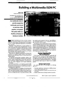
1 The mobile AR kit: (a) the single-processor system for simple targets; (b) the dualprocessor system for more complex scenarios; and (c) the AR kit in use. 54

(a)

November/December 2002

(b)

Miguel Ribo, Peter Lang, Harald Ganster, Markus Brandner, Christoph Stock, and Axel Pinz Graz University of Technology, Austria

(described in the sidebar “Related Work on AR Tracking Systems”), both components recover the full 6 DOF pose. Fusing the two tracking subsystems gives us the benefits of both technologies, while the sensors’ complementary nature helps overcome sensor-specific deficiencies. Our system is tailored to affordable, lightweight, energy-efficient mobile AR applications for urban environments, especially the historic centers of European cities.

Wearable AR kit Standard AR setups consist of either an optical or video see-through head-mounted display (HMD) to render graphics, a tracking device to follow the head position (indoor systems often use magnetic trackers), and a graphical workstation. To achieve mobility, a user must carry the AR setup, which limits its size, weight, and power consumption. Many commercially available wearable systems don’t have high-end 3D graphic chips and can’t support extra components (such as a framegrabber for cameras). Figure 1 shows our mobile AR kit, which consists of a real-time 3D visualization subsystem and a real-time tracking subsystem. The visualization subsystem uses a Dell Inspiron notebook (carried in a backpack) with a Geforce2Go graphics processor and Sony Glasstron high-resolution stereo HMDs with optical see-through capability (mounted to a helmet).

(c)

0272-1716/02/$17.00 © 2002 IEEE

Authorized licensed use limited to: University of Canterbury. Downloaded on August 03,2010 at 05:41:33 UTC from IEEE Xplore. Restrictions apply.

Related Work in AR Tracking Systems Several options for fully mobile tracking systems exist. In addition to vision-based and inertial tracking, developers have used the Global Positioning System (GPS), electronic compass, high-quality gyros, and several other sensors.1 Vision-based tracking can recover the full 6 DOF of a calibrated camera’s pose. Many vision-based tracking systems do this by solving the perspective n-point problem (PnP)2: Given n > 5 noncollinear points (landmarks) with known scene coordinates, the resulting camera pose is unique. PnP also works for the special case of n = 4 noncollinear, but coplanar landmarks. Vision-based tracking is too fragile to be used alone in an outdoor tracking system, however. Lines of sight can be temporarily blocked, motion can be blurred, or the field of view (FOV) can change rapidly, especially if users turn their heads quickly. A few hybrid systems track only 3 orientational DOF by combining gyros and vision.3,4 Yokokohji and colleagues combine vision with accelerometer information to predict head motion.5 Purely vision-based tracking is rarely achieved in real time,6 limited to a few selected landmarks (for example, one specific planar patch in the scene7), or restricted to unique scene models.8 Several recently proposed experimental hybrid systems for mobile outdoor AR tracking combine differential GPS (3 DOF position) and inertial tracking based on gyros and auxiliary sensors (3 DOF orientation).9–11

References 1. R.T. Azuma et al., “Tracking in Unprepared Environments for Augmented Reality Systems,” Computers and Graphics, vol. 23, no. 6, Dec. 1999, pp. 787-793.

We’ve used several prototype tracking subsystems. We can track simple targets and augment simple graphics using a single processor. In this case, we use a headmounted FireWire camera (640 × 480 pixels, color), which is easy to connect to the notebook (Figure 1a). For more demanding applications, we’ve developed a dual processor system with a dedicated single-board PC subsystem, which is also carried in the backpack (Figure 1b). This system uses either a FireWire camera or another camera/framegrabber configuration. Depending on camera type and scene complexity, the actual throughput of the visual tracking system varies from 10 to 60 Hertz. We developed the head-mounted inertial tracking device in our lab. It’s based on silicon micromachined accelerometers and gyroscopes, with a digital signal processor (DSP) to process sensor raw data and to communicate with the host computer. Update rates are greater than 500 Hz, which is an order of magnitude higher than for the vision-based system.

Tracking system We use the term “tracking” to describe real-time metric pose recovery from monocular video streams. The term is also used in calibration-free video aug-

2. C.P. Lu, G.D. Hager, and E. Mjolsness, “Fast and Globally Convergent Pose Estimation from Video Images,” IEEE Trans. Pattern Analysis and Machine Intelligence, vol. 22, no. 6, June 2000, pp. 610-622. 3. K. Satoh et al., “A Hybrid Registration Method for Outdoor Augmented Reality,” Proc. Int’l Symp. Augmented Reality, IEEE Computer Soc. Press, Los Alamitos, Calif., 2001, pp. 67-76. 4. S. You, U. Neumann, and R. Azuma, “Orientation Tracking for Outdoor Augmented Reality Registration,” IEEE Computer Graphics and Applications, vol. 19, no. 6, Nov./Dec. 1999, pp. 36-42. 5. Y. Yokokohji, Y. Sugawara, and T. Yoshikawa, “Accurate Image Overlay on Video See-through HMDs Using Vision and Accelerometers,” Proc. IEEE Virtual Reality 2000 (VR 2000), IEEE CS Press, Los Alamitos, Calif., 2000, pp. 247-254. 6. B. Jiang and U. Neumann, “Extendible Tracking by Line Auto-calibration,” Proc. IEEE and ACM Int’l Symp. Augmented Reality, IEEE CS Press, Los Alamitos, Calif., 2001, pp. 97-103. 7. V. Ferrari, T. Tuytelaars, and L. Van Gool, “Markerless Augmented Reality with A Real-Time Affine Region Tracker,” Proc. IEEE and ACM Int’l Symp. Augmented Reality, vol. I, IEEE CS Press, Los Alamitos, Calif., 2001, pp. 87-96. 8. A. Ansar and K. Daniilidis, “Linear Pose Estimation from Points or Lines,” Proc. European Conf. Computer Vision, vol. 4, A. Heyden et al., eds., Springer, Berlin, 2002, pp. 282-296. 9. W. Piekarski and B. Thomas, “Augmented Reality with Wearable Computers Running Linux,” Proc. 2nd Australian Linux Conf., Linux Australia, 2001, pp. 1-14. 10. T. Höllerer et al., “Exploring MARS: Developing Indoor and Outdoor user Interfaces to a Mobile Augmented Reality System,” Computers and Graphics, vol. 23, no. 6, Dec. 1999, pp. 779-785. 11. R.T. Azuma, “The Challenge of Making Augmented Reality Work Outdoors,” Mixed Reality: Merging Real and Virtual Worlds, chap. 21, Y. Ohta and H. Tamura, eds., Springer-Verlag, Berlin, 1999.

mentations based on the recovery of affine frames in images,2 a much simpler task than metric camera pose recovery. Accurate photorealistic 3D models exist for many cities, and developers are still working to increase their precision and realism. Our system uses such models in an offline process to extract promising visual landmarks. We use the resulting sparse model for real-time visionbased tracking. This model comprises a set of visual landmarks, or noncollinear points, which it describes using 2D images and the landmarks’ 3D position in the scene. The vision-based tracking component determines poses using the solution to the perspective n-point (PnP) problem (see the sidebar). For outdoor applications, we can’t focus on predefined artificial landmarks, but must find natural landmarks that the system can easily detect under varying lighting conditions and from different viewpoints. We prefer point-like features (such as corners), which we can find using an interest operator or corner detector in a small subwindow of the camera image. These operators detect significant local features, such as points with high spatial derivatives in more than one direction. The proposed tracking system consists of five dis-

IEEE Computer Graphics and Applications Authorized licensed use limited to: University of Canterbury. Downloaded on August 03,2010 at 05:41:33 UTC from IEEE Xplore. Restrictions apply.

55

Tracking

position. We illustrate these steps using a synthetic corner with known corner model (Figure 3a):

Sensor pool

2 Tracking system outline. A separate target selection process allows for contextdependent changes in the model database.

Test features Pose client

Pose

Selection Model features Hybrid tracker

Log/ response

Pose

Target selector

Commands Operator

tinct blocks, as Figure 2 shows. The hybrid tracker continuously delivers pose information—that is, the sensor’s pose with regard to the world coordinate system—to the pose client. To simplify correspondence, a target selector module preselects features from the model database in a context-dependent way. Thus, once initialization is complete, the system uses only subsets of the model database for tracking. Like the pose client, the target selector requires the actual pose information to maintain the active set of model features. However, target selector runs occur at a considerably lower rate (for example, 1 Hz) than the tracking loop. The hybrid tracker module has direct access to the sensor pool module, which holds the array of sensors and corresponding calibration data (one camera and an inertial sensor in our system). The operator can perform a number of maintenance and control tasks through the operator interface. The interfaces between adjacent modules in this design aren’t restricted to any distinct type. However, we primarily use transmission control protocol/Internet protocol (TCP/IP) connections for data communications, which lets us easily run different parts of the tracker on different CPUs.

Tracking corners Corners are significant features of an image that can serve as natural landmarks in tracking applications. Because corners are local features, tracking systems can compute them quickly, using only a small subset of the whole image. The main drawback of common corner detectors is the imprecise localization of the exact corner position. A localization error of a few pixels can lead to a significant position error (especially in depth) in 3D space, depending on the distance between the camera and the object. Therefore, we must improve the corner detector’s localization accuracy. Steinwendner, Schneider, and Bartl propose an edge detection method that uses spatial subpixel analysis for accuracy.3 Spatial subpixel analysis aims to estimate model parameters by analyzing the gray levels of the involved pixels within a small neighborhood. Our approach extends this work from edges to corners. Because corners are intersections of two or more edges that border different areas, we can use this approach to improve corner localization accuracy. It takes several steps to estimate the correct corner

56

1. Perform fast corner detection using a morphological approach.4 The cross in Figure 3b depicts the corner position that the morphological corner detector computed. This step is only necessary for the start frame and after reinitialization, otherwise the approximated corner position is predicted from previous frames. 2. Calculate the dominant gradient directions. We get a weighted density function by counting the gradient directions of all pixels in the 7 × 7 neighborhood of the estimated corner position and interpolating the results.5 Local maxima of the density function indicate the gradient directions of the involved edges. 3. Extract edge pixels within the estimated corner’s 7 × 7 neighborhood. The system selects all pixels with a sufficiently high gradient magnitude for further processing. These edge pixels are boundary pixels of adjacent regions. The boundary pixels in Figure 3b are labeled 1 to 5. 4. Compute line parameters using spatial analysis. The pixel value of each extracted edge pixel is a linear combination of the pure gray values of the adjacent regions. We compute the edge’s orientation α and offset d to the edge-pixel-center using Steinwendner, Schneider, and Bartl’s parameter model3 on a 3 × 3 neighborhood. These parameters describe the edge with subpixel accuracy. We formulate the optimization problem as follows: 9



∑ p i=1

original i

( )

− p d,α

estimated  i

2

 d,α min  →

(1)

where pioriginal denotes the original pixel value at position i and p(d,α)estimated denotes the pixel value at i position i originating from the estimated edge, which offset d and angle α describe. To decrease the computational cost of estimating the line parameters, we use the previously calculated dominant gradient directions as starting points for the optimization problem. 5. Remove wrong edge candidates. The parameter model we’ve described is inappropriate at pixels near the exact corner position because more than one edge exists within this neighborhood. This leads to wrong parameters for the edge model. We can remove the edges by comparing the angle α with the dominant gradient directions. Each edge that’s not aligned with one dominant gradient direction (calculated in a previous step) is removed. 6. Calculate the intersection point. Each intersection point for the remaining edges is a candidate for the exact corner position. These points vary only slightly. To further increase accuracy, we can calculate a consensus (for example, weighted average). Figure 3 shows the results of applying these processing steps to a synthetic (Figure 3b) and a real (Figure 3c) image.

November/December 2002 Authorized licensed use limited to: University of Canterbury. Downloaded on August 03,2010 at 05:41:33 UTC from IEEE Xplore. Restrictions apply.

(a)

(b)

(c)

Evaluating tracking features Vision-based tracking systems are unreliable unless they can identify and track good features from frame to frame.6 Thus, such systems must be able to select and track features that correspond to physical points of interest in the system’s surroundings. Our mobile tracking system deals with 2D point-like features, with an emphasis on corner localization (for example, T, Y, and X junctions) in image sequences, which a PnP algorithm (see the sidebar) uses to determine the system’s pose with respect to the environment. Because detection algorithms provide many point-like candidates, however, systems (especially for real-time applications) must extract ideal points of interest among the data. We’ve developed a technique to evaluate and monitor the quality of the detected and tracked image’s pointlike features. The basic strategy follows Shi and Tomasi’s6 measure function, but we also propose a broad use of the measure over the detected points. The measure function is defined by a 2 × 2 symmetric matrix, such that ∀p ∈ Image,  2  gx r  U p =  r∈Ω  g x r g y r 

() ∑ () () ()

 gx r g y r   2  gy r 

() () ()

(2)

where p = (x, y) is a detected image point under evaluation, r denotes a pixel in a 7 × 7 image window Ω centered at p and the functions gx(•) and gy(•) are gradient-based functions applied in x and y directions, respectively. Afterwards, the eigenvalues (λ1, λ2) of the matrix U for a given point p are computed and then used to build the feature vector V(p) defined by ∀p ∈ Image,   λ   µ p = min i    λ    i  ,i ∈ 1,2 V p =  max λ i   ρ p =   min λ i  

()

()

()

( ) ( )

{ }

(3)

We use the following evaluation criteria to find highquality points q among all possible corner candidates p: ■

3 Subpixel corner detection: (a) synthetic corner with plotted model; (b) recovered corner (synthetic image); and (c) recovered corner (real image).

Given a georeferenced 3D model M and a corresponding image sequence Si, the corner detector extracts the corners from each Si image. Then, as we

■

■

know the pose of all images in Si, we back-project all 3D points of M into these images to determine, among all detected corners, which image points are the projection of a 3D point. We label this set of corners Sc. For all points p in Sc, we compute the vector feature V(p) as defined in Equations 2 and 3. We also count how many times a point p appears in the sequence Si. We build the set of points Sp that contains all image points with an appearance value greater than or equal to two. Afterward, we select the “good points” Sq for a given pair (˜µ,˜ρ) such that

{

()

}

Sq = q ∈Sp V q ∈VBand ,

[() ] [( ) ]

[() ] [( ) ]

 ˜ ± 2 std µ p ≤ µ ˜  mean µ p ≤ µ p∈Sp  VBand =  p∈Sp  mean ρ p ≤ ρ ˜ ± 2 std ρ p ≤ ρ ˜    p∈Sp p∈Sp

(4)

where ˜µ and ˜ρ are threshold values used to eliminate sporadic high values of µ and ρ. Thus, a good point q is a point for which the vector feature V(q) remains similar (in accordance with Sq) during the whole image sequence Si. As a result, the system uses the detected and selected image points that satisfy the criteria to initialize itself (its pose, features to track, and the search windows from frame to frame). Moreover, the system can use these criteria to monitor and evaluate the “goodness” of the tracked image points during the tracking procedure. Figure 4 (next page) is an example of two tracked corners with two different goodness values: + indicates a good feature to track (that is, it satisfies Equation 4), while * indicates a bad feature to track (it doesn’t satisfy Equation 4).

Solving the correspondence problem Solving the PnP problem for a continuous sequence of input images requires establishing and maintaining correspondence between a set of image features and their model representations. In static scene analysis, this process is often referred to as pattern matching or object recognition. Complexity. The exponential complexity7 of finding a valid correspondence is not affordable for realtime operation. As the number of test features to be


57

Tracking

4 Two views of the same window (taken from sequence Si) with two tracked corners: + indicates a good feature to track, while * indicates a bad feature to track.

tracked increases, the time spent computing the correspondence on a per-frame basis will introduce an unacceptable lag into the system’s response. Tracking an object over time, however, lets the system maintain a set of corresponding features that change only slightly from one frame to the next. Changes occur primarily when the system loses track of a single feature (for example, after object occlusion or when the feature leaves the field of view) or when new features appear in the current FOV. This small difference assumption lets the system propagate knowledge from one correspondence module run to the next. In general, an outdoor AR application’s test feature set is a subset of the model feature set extended with spurious features (noise or real features) that are not included in the model. Additionally, the model feature set strongly depends on the current context (that is, the user’s position and activity within the AR environment). A separate target selection process handles context changes. This process continuously updates the model database depending on the application’s current context. The target selector initializes new features and removes features no longer in the FOV.

during correspondence search has an associated attribute vector A = [a1, a2, ..., an]. The elements of this vector denote geometric (such as location in the 3D scene) and other feature-dependent information (such as color). We denote the set of test features found in each tracker frame as F = [F1, F2, ..., FN] and the underlying model feature set as f = [f1, f2, ..., fM] . The interpretation tree can help us establish a list of feasible interpretations given both F and f. To avoid unnecessary computation during tree initialization, we apply a number of constraints based on the feature attributes ai, which are implemented as statistical hypothesis tests. Geometric constraints reflect the object’s geometry and the imaging system (the perspective invariants, for example). In the final structure, each tree node reflects a valid pairing of a model and a test feature, as Figure 5a (next page) shows. Although efficient heuristics limit the time spent during the correspondence search, this static interpretation tree doesn’t perform matching well enough to achieve real-time tracking. The Ditree extends the static interpretation tree, as Figure 5b shows, by the following processing steps: ■ Dynamic search ordering. For a valid interpretation,

Best-fit vs. multiple hypotheses. Apart from their computational complexity, pattern-matching algorithms usually deliver the correspondence between test and model data that fit best, rather than a list of feasible interpretations of the test data. Tracking applications, on the other hand, are likely to experience multiple correspondences, each of which has a similar probability of being the right one. A tracking algorithm’s ability to deal with numerous correspondence hypotheses is directly related to how the object dynamic is modeled. In systems based on Kalman filters,8 prediction can only track the best-fit correspondence over time. The system will discard any competing correspondence due to the unimodality of the Gaussian density as used by the Kalman filter approach. More recent developments show that one can simultaneously propagate a number of correspondence hypotheses over time, and thus switch between hypotheses as required.9 Dynamic interpretation tree. We extend Grimson’s interpretation tree structure7 toward a dynamic interpretation tree (Ditree)10 to achieve real-time behavior required for tracking applications. Each feature used

58

each test feature’s expected location will vary only slightly. Thus, we keep the interpretation tree structure from frame to frame and only update the test feature attributes. Test and model feature order is rearranged to reflect each interpretation’s quality-offit. Thus, strong hypotheses will appear at the beginning of the interpretation tree processing. These, together with the search heuristic and the cut-off threshold, are powerful mechanisms to keep the residual tree complexity (the number of leaf nodes) small. ■ Node management. New features Fi occurring in the image lead to the insertion of new nodes into the interpretation tree as in the static case. If required, the resultant tree can adapt to the scene and grow. Feature pairings that fail to conform to the set of constraints (for example, the attributes have changed too much between two consecutive tracker frames) must be removed from the tree. As in static trees, subtrees starting at an invalid feature pairing are removed. Thus, the tree is pruned whenever the system detects inconsistent features. ■ Feature recovery. Apart from delivering a list of valid feature pairings for every feasible interpretation, the


tree delivers the list of model features that haven’t been assigned successfully to a test feature and it can be used to recover those features. Assuming that missing features result from partial occlusion (which is true for simple features such as corners), the system can use this information to selectively search the subsequent input image for the missing features. The Ditree algorithm can deal with multiple hypotheses simultaneously through a set of Kalman filters. It uses the five strongest hypotheses to repeatedly update the corresponding filters. In a final processing step, the system applies a maximum likelihood scheme to identify the object pose for each tracker frame.

Test features

Feature preordering

Root Kalman filters ( ƒi –1, F1)

( ƒi , Fj )

( ƒi , FN )

Maximum likelihood estimator

( ƒi +1, Fm ) (a)

(b)

5 Interpretation trees. (a) Basic structure of the interpretation tree. Each node corresponds to a valid pairing of a model and a test feature. (b) Overview of the dynamic extensions to the interpretation tree.

Pose

Hybrid tracking Vision-based tracking systems often fail to follow fast motion, especially as the camera rotates. Our hybrid tracking system uses inertial sensors to overcome this drawback. Inertial tracking is fast but lacks long-term stability due to sensor noise and drift. Vision-based tracking, on the other hand, is highly precise and stable over the long term. Thus, we fuse sensors to exploit the complementary properties of the two technologies and to compensate for their respective weaknesses. Although commercially available inertial systems exist (such as those from Crossbow or Systron Donner), they’re too large, too heavy, too expensive, or deliver only three DOF (orientation only). We built a custom inertial tracker from single-axes micromachined inertial sensors (Figure 6). Our inertial tracker consists of three acceleration sensors with a range of ±5 g, three angular velocity sensors (gyroscopes) with a range of ±250 degrees per second, and measures acceleration as and angular velocity ωs in the three perpendicular sensor axes at 500 Hz. A DSP processes sensor raw data to correct sensor axes misalignment and communicates with the host computer. A modified Extended Kalman filter11 operating in a

6 Inertial tracker hardware. The main components are three accelerometers, three gyroscopes, and a DSP.

predictor-corrector manner implements sensor fusion, as Figure 7 shows. The state vector x maintains position p, velocity v, acceleration a, acceleration sensor bias ab, and orientation q. In the prediction step, we use the relative changes in position ∆p and orientation ∆q computed from inertial measurements ai and ωi to update ˆ in the temporal interthe new state vector estimation x val between two measurements from the vision-based tracker. In the measurement update step, we apply position pv and orientation qv to correct the state vector esti-

ˆ v, ˆ a, ˆ aˆ b, q ˆ p,

ωs a

s

Inertial tracker Coordinate transformation

ωi Prediction

Correction

ai

q

pv qv

Vision-based tracker

7 Fusion of vision-based and inertial tracker with a modified Extended Kalman filter.

p, v, a, ab, q


59

Tracking

(a)

(b)

(c)

8

Processing of a simple façade. (a) Snapshot from the video sequence. (b) Good corners Sq. The four points marked + are used for PnP pose calculation. (c) A simple augmentation of the scene as perceived by the user.

x (meters)

2 0

+ Inside-out – Hybrid

−2 −4 −6

0

2

4

6

8

10

12

14

0

2

4

6

8

10

12

14

y (meters)

−1.0 −1.5 −2.0 −2.4 −3.0 z (meters)

8 7 6 5

0

2

4

(a)

6 8 Time (seconds)

10

12

14

q0

−0.05

q1

0

2

4

6

8

10

12

14

0

2

4

6

8

10

12

14

2

4

6

8

10

12

14

2

4

6

8

10

12

14

1

q2

0.1 0.05 0 0

q3

0.5 0 −0.5 0 (b)

Time (seconds)

9

Tracking performance on the test sequence. The upper plots (a) show the translational components during user movement. The lower plots (b) are the corresponding quaternion data for the orientation components. The + symbol denotes the positions estimated by the vision-based tracker, whereas the line shows the tracked positions of the hybrid approach. Note the much finer scale for q0.

60

Experimental results To illustrate the performance of our wearable AR kit, we performed two experimental runs in outdoor situations of different complexity. Because ground-truth (the real trajectory of the user’s head in scene coordinates) is difficult to obtain and not available, we try to characterize system performance by analyzing real-time behavior, smoothness and plausibility of computed trajectories, and quality of 3D graphics augmentation.

Basic scenario

−0.1

−0.15

mation from the prediction step. In this manner we only rely on the inertial tracker between two vision-based updates and maintain the higher update rate from inertial tracking. The corrected orientation q is also used for the necessary coordinate transformation of the acceleration since position computation takes place in the world coordinate system and acceleration is measured in the moving coordinate system. Operating inertial and vision-based trackers on the same CPU allows for simple temporal synchronization between the two systems.

Figure 8 shows snapshots from a video sequence in which a user is moving toward and along an office building. We used a structure-from-motion approach to reconstruct the 3D model of the office facade and identified good features using the procedure described previously. Our reference coordinate system is in the upper left corner of the rightmost window in the window triplet shown in Figure 8, with the x-direction pointing right, y-direction pointing up, and z-direction perpendicular to the facade plane pointing toward the user. The test sequence is 13.5 seconds, with 403 image frames captured at a frame rate of 30 Hz. At the same time, the system captured the sensor data from our inertial tracking device at a rate of 500 Hz. Vision and inertial data streams are synchronized—that is, because they were captured in the same PC-platform, they share a common time basis, and we combine them within an Extended Kalman filter framework. Figure 9 shows the tracking precision during our test sequence. The user moved toward the building at an angle of approximately 45 degrees. The user looked left, then right, and then turned to the right, all of which is reflected by the decreasing z-values and the increasing x-values in the upper graphs (Figure 9a) and the changes in the orientation components of the lower graphs (Figure 9b).


(a)

(b)

10 Georeferenced 3D model. (a) 3D model with points of interest, roof lines, and camera positions (22 calibrated reference images). (b) Some of the images used to compute the 3D model. The model was provided by the VRVis Research Center for Virtual Reality and Visualization.12 The hybrid tracker delivers a much smoother tracking curve than the vision-based tracker module alone, which is especially evident in the position graphs in Figure 9a. In our fusion scheme, the vision-based tracking module confidence is higher than in the inertial component, so each vision-based update results in a correction of the state vector, which is clearly visible in Figure 9b. Furthermore, the hybrid approach keeps the advantages of both single tracker modules. The inertial tracker makes position and orientation data available at 200 Hz and above, while the vision-based tracking module generates the high precision. Several image frames contain too few features (under four) for the system to visually estimate a user’s position. This is due to the vision-based system’s low-level feature detection (for example, reflections can lead to incorrect corners and therefore the corners don’t fulfill the good-feature criterion) or, more likely, to the feature being outside the FOV. The inertial sensor data, however, lets the hybrid tracking device deliver reliable user positions over the complete test sequence. Figure 8 shows several snapshots from the original test video sequence. The view in Figure 8a is similar, but not identical to the user’s perception of the real scene as viewed through the semi-transparent HMD. Figure 8b shows the corners that were selected to be good features for tracking. The four corners of the rightmost window marked + were used for camera pose estimation. Figure 8c gives an impression, but is not identical to the user’s perception, of the real scene augmented with 3D graphics generated by the HMD.

of which are displayed in Figure 10b) to establish the 3D model. In an offline procedure, we extracted the most significant corners from the 22 images, which we then used for the actual tracking sequence. We performed the tracking sequence in the complex scenario using the dual-processor equipment (Figure 1b) and a charge-coupled device (CCD) camera capturing images at 60 Hz. The movement in this experimental run started with a rotation, which was followed by a translation along the facades. We used the interpretation tree method to select the features actually used for each tracking frame. For this complex scenario, the tracking algorithm must deal with several hundred significant corners, and inaccurate corner localization can lead to ambiguous landmark matching, complicating the correspondence problem and target selection. At the time of this writing, we’re close to, but haven’t yet reached, real-time performance using the dual-processor equipment. We show first results from a sequence that was captured in real time and processed offline. Figure 11 (next page) presents the tracking performance for the initial rotation (4-second sequence). Ferrari, Tuytelaars, and Van Gool performed similar experiements.2 Their work finds affine patches and augments a monocular video sequence. Our system measures the camera pose in 3D from a video sequence, but augments the real 3D view of the user with 3D graphics superimposed on an optical seethrough HMD. This is far more demanding in terms of accuracy and complexity.

Complex scenario

Conclusion

For the complex scenario, we used a complete georeferenced 3D model of a city section, shown in Figure 10a, to derive the most significant corners. We analyzed 22 calibrated high-resolution reference images (some

Our new hybrid tracking system can provide 6 DOF pose information in real-time. Experiments with an outdoor AR application have shown satisfactory system performance for a fairly simple scene. The tracking sub-


61

Tracking

q0

0.5 0 −0.5 0

+ Inside-out – Hybrid

0.5

1

1.5

0

2.5

3

3.5

4

4.5

0.5

1

1.5

0

2.5

3

3.5

4

4.5

0.5

1

1.5

0

2.5

3

3.5

4

4.5

0.5

1

1.5

0 2.5 Time (seconds)

3

3.5

4

4.5

Tracking performance on a part of the test sequence for the complex scenario. The plots show the quaternion data for the orientation components during user movement. The + symbol denotes the positions estimated by the visionbased tracker, whereas the line shows the tracked positions of the hybrid approach.

0 −0.5 0 0.5

q2

11

q1

0.5

0.6 −0.7 0

q3

0.8 0.7 0.6 0

system can deliver its pose measurements to any pose client and thus can be used in many potential navigation scenarios. Future work will explore complementary metal-oxide semiconductor (CMOS) camera technology to directly address small windows holding visual landmarks. This will lead to significantly higher frame rates of several hundred Hertz. CMOS cameras also offer higher spatial resolution, so we can obtain more precise corner localization. We plan to further extend the combination of corners and supporting edges to compound features, which will describe a visual landmark in more detail. This again will gain precision and will also reduce the complexity of visual search, so fairly complex scenarios, such as those in Figure 10, will be manageable in real-time. Finally, we plan to build an AR system using two cameras. The CMOS camera will be used for precise insideout tracking of 6 DOF of the user’s head, while the FireWire camera will track the user’s hands and gestures for 3D interaction in the near field.

Acknowledgments We gratefully acknowledge support from the following projects: Christian Doppler Laboratory for Automotive Measurement Research, the Mobile Collaborative Augmented Reality project (MCAR, Austrian “Fonds zur Förderung der wissenschaftlichen Forschung” project number P14470-INF), and Vampire: Visual Active Memory Processes and Interactive Retrieval (EU-IST Programme -IST-2001-34401). We wish to thank the VRVis Research Center for Virtual Reality and Visualization research area AR 2: Virtual Habitat under the supervision of Konrad Karner for providing the georeferenced 3D data set used in Figure 10.

62

References 1. S.K. Feiner, “Augmented Reality: A New Way of Seeing,” Scientific American, vol. 4, 2002. 2. V. Ferrari, T. Tuytelaars, and L. Van Gool, “Markerless Augmented Reality with a Real-Time Affine Region Tracker,” Proc. IEEE and ACM Int’l Symp. Augmented Reality, vol. I, IEEE Computer Soc. Press, Los Alamitos, Calif., 2001, pp. 87-96. 3. J. Steinwendner, W. Schneider, and R. Bartl, “Subpixel Analysis of Remotely Sensed Images,” Digital Image Analysis: Selected Techniques and Applications, chap. 12.2, W.G. Kropatsch and H. Bischof, eds., Springer-Verlag, New York, 2001, pp. 346-350. 4. R. Laganiere, “Morphological Corner Detection,” Proc. IEEE Int’l Conf. Computer Vision, IEEE CS Press, Los Alamitos, Calif., 1998, pp. 280-285. 5. S. Yin and J.G. Balchen, “Corner Characterization by Statistical Analysis of Gradient Directions,” Proc. Int’l Conf. Image Processing, vol. 2, IEEE CS Press, Los Alamitos, Calif., 1997, pp. 760-763. 6. J. Shi and C. Tomasi, “Good Features to Track,” Proc. IEEE Conf. Computer Vision and Pattern Recognition, IEEE CS Press, Los Alamitos, Calif., 1994, pp. 593-600. 7. W.E.L. Grimson, Object Recognition by Computer: The Role of Geometric Constraints, MIT Press, Cambridge, Mass., 1990. 8. C. Harris, “Tracking with Rigid Models,” Active Vision, A. Blake and A. Yuille, eds., MIT Press, Cambridge, Mass., 1992, pp. 59-73. 9. M. Isard and A. Blake, “ICONDENSATION: Unifying Lowlevel and High-level Tracking in a Stochastic Framework,” Proc. European Conf. Computer Vision, vol. 1, Lecture Notes in Computer Science 1406, Springer-Verlag, Berlin, 1998, pp. 893-908.


10. M. Brandner and A. Pinz, “Real-time Tracking of Complex Objects Using Dynamic Interpretation Tree,” Pattern Recognition, Proc. of 24th DAGM Symp., Lecture Notes in Computer Science 2449, Springer-Verlag, Berlin, 2002, pp. 9-16. 11. G. Welch and Gary Bishop, “SCAAT: Incremental Tracking with Incomplete Information,” Computer Graphics, T. Whitt, ed., Addison-Wesley, Reading, Mass., 1997, pp. 333344. 12. A. Klaus et al., “MetropoGIS: A Semi-automatic City Documentation System,” Proc. Photogrammetric Computer Vision 2002 (PCV02)—ISPRS Commission III Symp., vol. A, Int’l Soc. for Photogrammetry and Remote Sensing (ISPRS), 2002, pp. 187-192.

Miguel Ribo is a senior researcher at the Christian Doppler Laboratory for Automotive Measurement Research at Graz University of Technology. His research interests include real-time machine vision, autonomous robot navigation, data fusion, spatial representation, and augmented reality. He received the DEA diploma in computer vision, image processing, and robotics from the University of Nice-Sophia Antipolis, France, and a PhD in computer engineering from Graz University of Technology.

Peter Lang is a research staff member at the Institute of Electrical Measurement and Measurement Signal Processing at Graz University of Technology. His research interests are in digital signal processing with a special focus on sensor fusion. He received an MS in telematics from the Graz University of Technology.

Harald Ganster is a senior researcher at the Graz University of Technology Institute of Electrical Measurement and Measurement Signal Processing. His research interests are computer vision, image analysis, and augmented reality. His current

research topic is vision-based tracking, with special focus on mobile application. He received an MSc and a PhD in mathematics from the Graz University of Technology, Austria.

Markus Brandner is working toward a PhD degree in the field of hybrid tracking for real-time applications. He received an MS in telematics (computer engineering) from Graz University of Technology.

Christoph Stock is a research staff member at the Institute of Electrical Measurement and Measurement Signal Processing at Graz University of Technology. He received an MS in telematics from the Graz University of Technology. His research interests are in computer vision and augmented reality with a special focus on visual tracking applications.

Axel Pinz is an associate professor at Graz University of Technology, Institute of Electrical Measurement and Measurement Signal Processing. His research interests are cognitive vision, object recognition, and information fusion, as well as real-time vision with applications in robotics, augmented reality, medical image analysis, and remote sensing. He received an MSc in electrical engineering and a PhD in computer science from Vienna University of Technology, and the Habilitation in Computer Science from Graz University of Technology, Austria. Pinz is a member of the IEEE, and chair of the Austrian Association for Pattern Recognition (AAPR). Readers may contact Axel Pinz at the Inst. of Electrical Measurement and Measurement Signal Processing, Univ. of Technology, Graz, Kopernikusgasse 24, A-8010 Graz, Austria, email [email protected]. For further information on this or any other computing topic, please visit our Digital Library at http://computer.org/publications/dlib.


63