Mar 30, 2009 - build state-based scheduling control loops as depicted in section 6.2. .... Any practical feedback system is designed to obtain some stability ..... approach has been used in the framework of the so-called (m,k)-firm .... The design basics and ..... Note that the processor also executes the robot arm numerical ...
GRANT AGREEMENT N˚223866
Deliverable D04.01 Report Nature Dissemination Public
D04.01 - State of the art in control/computing co-design Report Preparation Date 30/MAR/2009 updated 30/JUL/2009 Project month: 6 Authors
Daniel Simon, NeCS-INRIA and Alexandre Seuret NeCS-CNRS Peter Hokayem and John Lygeros, ETH Eduardo Camacho, US
Report Version Doc ID Code Contract Start Date Duration Project Coordinator :
V2 INRIACO01_D04.01_30JUL2009_V2 01/09/2008 36 months Carlos CANUDAS DE WIT, INRIA, France
Theme 3: Information and Communication Technologies
Control and Computing Co-design - D04.01
SUMMARY
In this report some methodologies for control and scheduling co-design are reviewed. Although control and real-time computing co-exist since several decades, control and computer scientists and engineers traditionally work in a cascaded way under separation of concerns : this approach leads to misunderstand many constraints and requirements concerning the implementation of control loops on real-time and distributed architectures. A very common misconception considers that control systems are "hard real-time", i.e. that they cannot suffer timing disturbance such as jitter or missing data. Indeed closed-loop systems are, to some extend, inherently robust to uncertainties, including implementation induced timing deviations : this property could be further enhanced to design controllers to be weakly timing sensitive and to accommodate for specified timing uncertainties. Relaxing the usual fixed sample rate and delays assumptions also allows for closed-loop scheduling control where the controller scheduling parameters are on-line adapted w.r.t. the measured computer activity while keeping the system stability. Thus variable sampling or asynchronous control can be used to automatically constrain the CPU or network bandwidth inside specified bounds under weakly known operating conditions. Considering the variety of plant models, computing architectures and associated constraints found across case studies, a large part of the current control tool-box can be adapted and reused for this purpose. On the other hand some other more extreme methods, such as event based control, can be designed to better cope with the asynchronous and timely sporadic nature of real-life systems. Indeed beyond the design of timely robust control laws on one hand, and the implementation of control aware feedback schedulers on the other hand, the problem in the large can be stated as "optimizing a control performance under implementation constraints" : up to now this problem only has partial answers based on case studies and particular configurations. Due the complexity and uncertainty of real life control systems, finding such general solutions is out of the scope of the project. Hence the ongoing research in FeedNetBack WP4 will focus on two promising directions : • Variable sampling based on LPV/H∞ control, as described in section 5.2, provides a way of preserving the stability and requested performance level of linear systems whatever are the variations of the control period inside prescribed bounds. The method based on polytopic models has a low complexity, allowing an easy implementation on a real-time target. However it is up to now limited to the case where the sampling rate is the only variable parameter in the plant model. Other LPV based robust control methods, such as gridding and LFT, will be investigated to handle both timing and plant model parameters variations. However the current method provides a safe platform to build state-based scheduling control loops as depicted in section 6.2. The properties and timing related performance of such variable sampling control laws deserve to be further studied, so that they can be further combined with an appropriate outer scheduling controller, to ensure both the stability of the controlled process and the efficiency of the execution resources sharing. • The previous methods only provide a limited way for handling non-linearities. On the other hand Model Predictive Control, as described in section 5.3, naturally deals with non-linear plants and controllers. However it usually suffers from an high computational complexity which is not compliant with limited computation power and restrict its use for slow dynamic systems. In particular 2
Control and Computing Co-design - D04.01 co-designing control and computing over distributed architecture, using MPC design, up to now received poor attention. The way in which MPC can be applied to the Control and Computing Co-Design problem will be investigated. The research will include topics such as how to implement MPC in a distributed manner taking into account the computation capability of the nodes. Techniques such as multi parametric MPC in a distributed context, approximations and the necessary MPC robustification will be studied. Current methods for distributed MPC have relied on the use of input-to-state stability coupled with a generalized small-gain condition as a way of designing robust controllers for distributed, networked systems. However, these methods suffer from conservativeness. We shall investigate the possibility of alleviating this conservativeness through the use of iterative redesign schemes and scheduled communication among the subsystems. As part of WP4 of the FEEDNETBACK project we shall also investigate approximate explicit MPC methods (based for example on wavelet theory), which require less storage and on-line searching, but provide stability and performance guarantees comparable to those of the exact explicit MPC schemes.
3
Control and Computing Co-design - D04.01
Contents 1
Introduction
2
Control and Computing Constraints 2.1 Digital Control of Continuous Systems 2.2 Control and Timing Uncertainty . . . 2.3 Accelerable control tasks . . . . . . . 2.4 Control and Scheduling . . . . . . . .
5
. . . .
. . . .
. . . .
. . . .
. . . .
. . . .
. . . .
. . . .
. . . .
. . . .
. . . .
. . . .
. . . .
. . . .
. . . .
. . . .
. . . .
. . . .
. . . .
. . . .
. . . .
. . . .
. . . .
. . . .
. . . .
. . . .
. . . .
5 5 6 7 7
3
Computing with control constraints in mind 8 3.1 Off-line approaches . . . . . . . . . . . . . . . . . . . . . . . . . . . . . . . . . . . . . 8 3.2 Scheduling Parameters Assignment . . . . . . . . . . . . . . . . . . . . . . . . . . . . 10
4
Feedback Scheduling Basics 4.1 Control of the Computing Resource . . . . . . . . . . . . . . 4.2 Control Structure . . . . . . . . . . . . . . . . . . . . . . . . 4.3 Sensors and Actuators . . . . . . . . . . . . . . . . . . . . . . 4.4 Control Design and Implementation . . . . . . . . . . . . . . 4.5 P.I.D. feedback scheduler for a web server . . . . . . . . . . . 4.6 LQG based feedback scheduling . . . . . . . . . . . . . . . . 4.7 Adaptive Scheduling of a Robot Controller : a Feasibility study 4.7.1 Plant Modelling and Control Structure . . . . . . . . . 4.7.2 Scheduling Controller Design . . . . . . . . . . . . . 4.7.3 Implementation of the Feedback Scheduler . . . . . .
5
6
Control under computations constraints 5.1 Robust control w.r.t. latencies and delays . . . . . . . . . 5.1.1 Overview . . . . . . . . . . . . . . . . . . . . . 5.1.2 Delay models . . . . . . . . . . . . . . . . . . . 5.1.3 Stability analysis of TDS using Lyapunov theory 5.1.4 Conclusion . . . . . . . . . . . . . . . . . . . . 5.2 LPV/H∞ synthesis of a sampling varying controller . . . 5.2.1 Performance specification . . . . . . . . . . . . 5.2.2 LPV/H∞ control design . . . . . . . . . . . . . 5.3 Model Predictive Control . . . . . . . . . . . . . . . . . 5.3.1 MPC and asynchrony . . . . . . . . . . . . . . . 5.3.2 Distributed MPC . . . . . . . . . . . . . . . . .
. . . . . . . . . . .
. . . . . . . . . . .
. . . . . . . . . . .
. . . . . . . . . .
. . . . . . . . . . .
. . . . . . . . . .
. . . . . . . . . . .
. . . . . . . . . .
. . . . . . . . . . .
. . . . . . . . . .
. . . . . . . . . . .
. . . . . . . . . .
. . . . . . . . . . .
. . . . . . . . . .
. . . . . . . . . . .
. . . . . . . . . .
. . . . . . . . . . .
. . . . . . . . . .
. . . . . . . . . . .
. . . . . . . . . .
. . . . . . . . . . .
. . . . . . . . . .
. . . . . . . . . . .
. . . . . . . . . .
. . . . . . . . . . .
. . . . . . . . . .
. . . . . . . . . . .
. . . . . . . . . .
. . . . . . . . . . .
. . . . . . . . . .
10 12 12 12 13 14 15 18 18 18 19
. . . . . . . . . . .
21 21 21 25 27 30 30 31 32 33 33 34
Joint control and computing design 35 6.1 MPC based feedback-scheduler . . . . . . . . . . . . . . . . . . . . . . . . . . . . . . . 35 6.2 Elastic scheduling and robust control . . . . . . . . . . . . . . . . . . . . . . . . . . . . 36 6.3 Convex Optimization Approach to Feedback Scheduling . . . . . . . . . . . . . . . . . 37
4
Control and Computing Co-design - D04.01 7
Summary and further work
1
Introduction
37
Digital control systems can be implemented as a set of tasks running on top of an off-the-shelf realtime operating system (RTOS) using fixed-priority and preemption. The performance of the control, e.g measured by the tracking error, and even more importantly its stability, strongly relies on the values of the sampling rates and sensor-to-actuator latencies (the latency we consider for control purpose is the delay between the instant when a measure qn is taken on a sensor and the instant when the control signal U (qn ) is received by the actuators((Åström and Wittenmark 1997)). Therefore, it is essential that the implementation of the controller respects an adequate temporal behaviour to meet the expected performance. However implementation constraints such as multi-rate sampling, preemption, synchronisation and various sources of delays make the run-time behaviour of the controller very difficult to accurately predict. However as we deal with closed-loop controllers we may take advantage of the robustness of such systems to design and implement flexible and adaptive real-time control architectures. This report reviews some robust and adaptive solutions for real-time scheduling and control co-design. Firstly we review some properties of closed-loop controllers in contrast with real-time implementation constraints. Some recent results in control and scheduling co-design, based on off-line strategies, are recalled in section 3. The main structures of feedback schedulers are given, and a few examples are detailed. Future research directions are sketched to conclude the paper.
2
Control and Computing Constraints
Closed-loop digital control systems use a computer to periodically sample sensors, compute a control law and send control signals to the actuators of a continuous time physical process. The control algorithm can be either designed in continuous time and then discretized or directly synthesised in discrete time taking account of a model of the plant sampled by a zero-order holder. Control theory for linear systems sampled at fixed rates has been established a long time ago, e.g. (Åström and Wittenmark 1997). Assigning an adequate value for the sampling rate is a decisive duty as this value has a direct impact on the control performance and stability. While an absolute lower limit for the sampling rate is given by Shannon’s theorem, in practise rules of thumb are used to give a useful range of control frequencies according to the process dynamics and to the desired closed-loop bandwidth (see for example section 4.7.2). A common observation is that lower are the control period and latencies, better is the control performance (e.g. measured by the tracking error or disturbances rejection1 ). 2.1
Digital Control of Continuous Systems
To implement a controller, the basic idea consists in running the whole set of control equations in a unique periodic real-time task whose clock gives the controller sampling rate. In fact, all parts of the control algorithm do not have an equal weight and urgency w.r.t. the control performance. To minimise the latency, a control law can be basically implemented as two real-time blocks, the urgent one sends the control signal directly computed from the sampled measures, while updating the state estimation or parameters can be delayed or even more computed less frequently (Åström and Wittenmark 1997). In fact, a complex system involves sub-systems with different dynamics which must be further coordinated (Törngren 1998). Assigning different periods and priorities to different blocks according to 1
This assumption can be enforced by providing a suitable control parameters tuning, as discussed in section 2.3
5
Control and Computing Co-design - D04.01 their relative weight allows for a better control of critical latencies and for a more efficient use of the computing resource (Simon, Castillo and Freedman 1998). However in such cases finding adequate periods for each block is out of the scope of current control theory and must be done through case studies, simulation and experiments. Latencies have several sources : the first one comes from the computation duration itself, and worst case execution times are difficult to get. In multi-tasking systems they come from preemption due to concurrent tasks with higher priority, from precedence constraints and from synchronisation. Another source of delays is the communication medium and protocols when the control system is distributed on a network of connected devices. In particular it has been observed that in synchronous multi-rate systems the value of sampling-induced delays show complex patterns and can be surprisingly long (Wittenmark 2001). 2.2
Control and Timing Uncertainty
While timing uncertainties have an impact on the control performance they are difficult to be accurately modelled or constrained to lie inside precisely known bounds. Thus it is worth examining the sensitivity of control systems w.r.t. timing fluctuations. Control systems are often cited as examples of "hard real-time systems" where jitter and deadline violations are strictly forbidden. In fact experiments show that this assumption may be false for closedloop control. Any practical feedback system is designed to obtain some stability margin and robustness w.r.t. the plant parameters uncertainty. This also provides robustness w.r.t. timing uncertainties : closedloop systems are able to tolerate some amount of sampling period and computing delays deviations, jitter and occasional data loss with no loss of stability or integrity. For example in (Cervin 2003) the loss of control performance has been checked experimentally using an inverted pendulum, for which a LQ controller has been designed according to a nominal sampling period and null delay and jitter. Figure 1 show the output performance (position error variance) when respectively the period, the I/O latency and the output jitter are increased : the controller behaviour can still be considered as correct as long as the sample-induced disturbances stay inside the performance specification bounds.
Figure 1. Performance loss w.r.t. timing deviations
Therefore the hard real-time assumption must be softened to better cope with the reality of closed-loop control. For example they can be changed for "weakly hard" constraints : absolute deadlines are replaced by statistical ones, e.g. the allowable output jitter compliant with the desired control performance or the number of allowed deadlines miss over a specified time window (Bernat, Burns and Llamosí 2001). Note that to be fully exploited, weakly hard constraints should be associated with a decisional process : 6
Control and Computing Co-design - D04.01 tasks missing their deadline can be for example delayed, aborted or skipped according to their impact on the control law behaviour, e.g. as analysed in (Cervin 2005). Finding the values of such weakly hard constraints for a given control law is currently out of the scope of current control theory in the general case. However the intrinsic robustness of closed-loop controllers allows for complying with softened timing constraints specification and flexible scheduling design. 2.3
Accelerable control tasks
A common assumption about the sampling rate of control tasks is that faster is the computation and better is the result, i.e. that control tasks are always accelerable. This fact has been for example observed in robot control, as in (Jaritz and Spong 1996). Stability robustness against deviations of the control period around a nominal value has been investigated in (Palopoli, Pinello, Sangiovanni-Vincentelli, Elghaoui and Bicchi 2002) where a stability radius around nominal periods is computed for a set of scalar systems. However recent investigations (Ben Gaid, Simon and Sename 2008b) revisited the common assumption, and suggest that only relying on robustness is not enough to preserve the control performance, and that adaptation w.r.t. the actual control period is almost always better. An accelerable control task has the property that more executions are performed, better is the control performance. When used in conjunction with weakly-hard real-time scheduling design, an accelerable control task allows taking advantage of the extra computational resources that may be allocated to it, and to improve the control performance with respect to worst case design methods. In practice, however, control laws designed using standard control design methods (assuming a periodic sampling and actuation) are not necessarily accelerable. Case studies have shown that, when a control law is executed more often than allowed by the worst case execution pattern (with no gains adaption), the performance improvement may be state dependent, and that performance degradation can be observed. Conditions for the design of accelerable tasks has been established, based on Bellman optimality principle, in the framework of a (m,k)-firm scheduling policy. Is is assumed that an optimal control law exists in the case of the worst case execution sequence, i.e. when only the mandatory instances of the control task are executed to completion. It is shown that, in the chosen framework, it is possible to systematically design accelerable control laws, which control performance increases when more instances of the control task can be executed during the free time slots of the system. The theory is quite general and does not require the process linearity. 2.4
Control and Scheduling
From the implementation point of view, real-time systems are usually modelled by a set of periodic tasks assigned to one or several processors and a worst case response times technique is used to analyse fixed-priority real-time systems. Well known scheduling policies, such as Rate Monotonic for fixed priorities and EDF for dynamic priorities, assign priorities according to timing parameters, respectively sampling periods and deadlines. They are said to be "optimal" as they maximise the number of tasks sets which can be scheduled with respect of deadlines, under some restrictive assumptions ((Audsley, Burns, Davis, Tindell and Wellings 1995, Sha, Abdelzaher, Årzén, Cervin, Baker, Burns, Buttazzo, Caccamo, Lehoczky and Mok 2004)). Unfortunately they are not optimised for control purpose. They hardly take into account precedence and synchronisation constraints which naturally appear in a control algorithm. The relative urgency or criticality of the control tasks can be unrelated with the timing 7
Control and Computing Co-design - D04.01 parameters. Thus, the timing requirements of control systems w.r.t. the performance specification do not fit well with scheduling policies purely based on schedulability tests. It has been shown through experiments, e.g. (Cervin 2003), that a blind use of such traditional scheduling policy can lead to an inefficient controller implementation; on the other hand a scheduling policy based on application’s requirements, associated with a right partition of the control algorithm into real-time modules may give better results. It is often the case that improving some computing related features is in contradiction with another one targeted to improve the control behaviour. For example the case studies examined in (Buttazzo and Cervin 2007) show that an effective method to minimise the output control jitter consists in systematically delaying the output delivery at the end of the control period : however this method also introduces a systematic one period input/output latency and therefore most often provides the worst possible control performance among the set of studied strategies. Another example of unsuitability between computing and control requirements arises when using priority inheritance or priority ceiling protocols to bypass priority inversion due to mutual exclusion, e.g. to ensure the integrity of shared data. While they are designed to avoid dead-locks and minimise priority inversion lengths, such protocols jeopardise at run-time the initial schedule which was carefully designed to meet control requirements. As a consequence latencies along some control paths can be largely increased leading to a poor control performance or even instability. Finally off-line schedulability analysis rely on a right estimation of the tasks worst case execution time. Even in embedded systems the processors use caches and pipelines to improve the average computing speed while decreasing the timing predictability. Another source of uncertainty may come from some pieces of the control algorithm. For example, the duration of a vision process highly depends on incoming data from a dynamic scene. Also some algorithms are iterative with a badly known convergence rate, so that the time before reaching a predefined threshold is unknown (and must be bounded by a timeout). In a dynamic environment, some control activities can be suspended or resumed and control algorithms with different costs can be scheduled according to various control modes leading to large variations in the computing load. Thus real-time control design based on worst case execution time, maximum expected delay and strict deadlines inevitably leads to a low average usage of the computing resource and to a poor adaptivity w.r.t. a complex execution environment. All these drawbacks call for a better integration of control goals and computing capabilities through a co-design approach.
3
Computing with control constraints in mind
3.1
Off-line approaches
A first set of methods consists in computing off-line the set of scheduling parameters which (ideally) maximise the control performance under schedulability constraints. The first step consists in getting a model of the control performance function of the execution parameters. The problem of optimal sampling period selection, subject to schedulability constraints, was first introduced in (Seto, Lehoczky, Sha and Shin 1996). Considering a bubble control system benchmark, the relationship between the control cost (corresponding to a step response) and the sampling periods were approximated using convex exponential functions. Using the Karush-Kuhn-Tucker (KKT) first order optimality conditions, the analytic expressions of the optimal off-line sampling periods were established. The problem of the joint optimisation of control and off-line scheduling has been studied in (Rehbinder and Sanfridson 2004, Lincoln and Bernhardsson 2002, Gaid, Çela, Hamam and Ionete 2006). 8
Control and Computing Co-design - D04.01 Other approaches define a Quality of Service criterion to depict, e.g., the relations between the performance and the controller’s period. This performance model can be used to configure an admission controller managing the overall system load ((Abdelzaher, Atkins and Shin 1997)) or the perform an on-line negotiation on periods and priorities as in (Sanfridson 2000). In a multitasking system several control tasks share a common computing resource : the resulting preemption induces latencies dues to the computations themselves, but also due to the interleaving between their executions. Models of the control behaviour based on linear systems theory is used in (Ryu, Hong and Saksena 1997) and (Saksena, Ptak, Freedman and Rodziewicz 1998) to derive cost functions which depict the control performance, e.g. the rise time, as a function of two execution parameters, the control period and loop delay. Then an optimisation iterative algorithm (simplex) is used to tune the execution parameters, in order to maximise the overall control performance with respect of the implementation feasibility. However due to the complexity of the optimisation process this method can be used only off-line. Often the lazy way to implement a controller consists in programing a single real-time task when all the components of the controller are executed in sequence in a single loop. However it appears that all the components of a control algorithm do not require the same timing parameters, and do not have the same weight in the final performance and stability. Some part of the controller are more critical w.r.t. latencies, or require more frequent updating than others. Therefore the controller can be split into modules according to these timing requirements, so that latencies can be minimised along some critical data paths, or so enforce the execution of safety critical functions even in case of transient overload. For example it is possible to partition the controller of a linear system as shown in (Åström and Wittenmark 1997) : while(1){ Wait-Clock A/D-Conversion Calculate-Output u(k) = f (y(k), xˆ(k − 1), ...) D/A-Conversion Update-State xˆ(k) = g(y(k), xˆ(k − 1), ...) } Here the input/output latency is minimised, where the commands are immediately computed after updating the measures, while updating the model and internal state of the controller can be delayed until the end of the control period. This method is for example used in (Eker and Cervin 1999) where this control tasks split is applied to the control of a set of concurrent inverted pendulums : it provides an impressive increase in the control performance with no additional computing cost. In more complex and non-linear system can also benefit of such separation of the control algorithm between fast and critical control paths (e.g. low level stabilisation loop) and slower components, e.g. vision based navigation. Obviously the operating system and associated run-time framework must allow for such multi-tasks/multi-rate implementation (Simon and Benattar 2005). This modular timing analysis seems to be an essential starting point for flexible and efficient real-time control implementation, as in the example depicted in section 4.7 Besides control considerations, flexible and control aware solutions also have been provided by the computer science side. For example let us cite the “Elastic Tasks” paradigm (Buttazzo and Abeni 2000), 9
Control and Computing Co-design - D04.01 where the sensitivity of the QoS (Quality of Service) relative to the execution period for every tasks is modelled by a “stiffness” and takes account bounds in the allowed execution period. To make the tasks set schedulable, the tasks stack is “compressed” until the accumulated execution load fit with the allocated CPU capacity. Although this implementation is in open loop w.r.t. the actual QoS it allows for an improved adaptation against transients overloads. Let us cite also the Control-Server ((Cervin and Eker 2003)) where a fraction of the total CPU power is statically reserved to each control thread. Then the systems behaves as if each controller was isolated using its own computation resource, in particular an overloaded controller do not disturb its neighbours. Inside each computing segment the individual controllers are organised to minimise their I/O latency and jitter. In case of transient overload the missing computing budget for one controller is reported to its next reserved slice, with no impact on the others. 3.2
Scheduling Parameters Assignment
This mainly concerns the integration of control performance knowledge in the scheduling parameters assignment. Indeed, once a control algorithm has been designed, a first job consists in assigning timing parameters, i.e. periods of tasks and deadlines, so that the controller’s implementation satisfies the control objective. This may be done off-line or on-line. In off-line control/scheduling co-design setting adequate values for the timing parameters rapidly falls into case studies based on simulation and experiments. For instance in (Ryu et al. 1997) off-line iterative optimisation is used to compute an adequate setting of periods, latencies and gains resulting in a requested control performance according to the available computing resource and implementation constraints. Also in (Sandström and Norström 2002) the temporal requirements of the control system are described using complex temporal attributes (e.g. nominal period and allowed variations, precedence constraints. . . ) : this model is then used by an off-line iterative heuristic procedure to assign the scheduling parameters (e.g. priorities and offsets) to meet the constraints. Concerning co-design for on-line implementation, recent results deal with varying sampling rates in control loops in the framework of linear systems : for example (Schinkel, Chen and Rantzer 2002) show that, while switching between two stable controllers, too frequent control period switches may lead to unstability. Unfortunately most real-life systems are non-linear and the extrapolation of timing assignment through linearisation often gives rough estimations of allowable periods and latencies or even can be meaningless. In fact, as shown later in the examples, the knowledge of the plant’s behaviour is necessary to get an efficient control/scheduling co-design.
4
Feedback Scheduling Basics
Besides traditional assignment of fixed scheduling parameters, more flexible scheduling policies have been investigated. Let us cite e.g. (Buttazzo and Abeni 2000) where the elasticity of the tasks’ periods enables for controlling the quality of service of the system as a function of the current estimated load. While such an approach is still working in open loop w.r.t. a controlled plant, the on-line combination the control performance and implementation constraints lead to the feedback scheduling approach. This approach has been initiated both from the real-time computing side (Lu, Stankovic, Tao and Son 2002) and from the control side (Cervin and Eker 2000, Eker, Hagander and Arzen 2000, Cervin, Eker, Bernhardsson and Arzen 2002). The idea consists in adding to the process controller an outer sampled feedback loop ("scheduling regulator") to control the scheduling parameters as a function of a QoC (Quality of Control) measure. It is expected that an on line adaption of the scheduling parameters 10
Control and Computing Co-design - D04.01 of the controller may increase its overall efficiency w.r.t. timing uncertainties coming from the unknown controlled environment. Also we know from control theory that closing the loop may increase performance and robustness against disturbances when properly designed and tuned (otherwise it may lead to instability). plant modelling and actual QoCs CPU/network state
Global objective
load/latency estimates Instrumentation
Scheduling Manager
QoS +
Scheduling
−
RTOS
Controller
feedforward admission controller exceptions handling
Scheduler Scheduling Parameters
Process objectives (QoC)
+
Process Controller
−
SAMP
Uk
ZOH
Process
Y
Process state estimates
Figure 2. Hierarchical control structure
Figure 2 gives an overview of a feed-back scheduler architecture where an outer loop (the scheduling controller) adapts in real-time the scheduling parameters from measurements taken on the computer’s activity, e.g. the computing load2 . Besides this controller working periodically (at a rate larger than the sampling periods of the plant control tasks), the system’s structure may evolve along a discrete time scale upon occurrence of events, e.g. for new tasks admission or exception handling. These decisional processes may be handled by another real-time task, the scheduling manager, which is not further detailed in this paper. Notice that such a manager may give a reference to the controller resource utilisation. The design problem can be stated as control performance optimisation under constraint of available computing resources. Early results come from (Eker et al. 2000) where a problem of optimal control under computation load constraints is theoretically solved by a feedback scheduler, but leads to a solution too complex to be implemented in real-time. Then (Cervin 2003) shows that this optimal control problem can be often simply implemented by computing the new tasks periods by the rescaling : hk+1 = hki i
U Usp
where Usp is the utilisation set-point and U the estimated CPU load. The feedback scheduler then controls the processor utilisation by assigning task periods that optimise the overall control performance. This approach is well suited for a "quasi-continuous" variation of the sampling periods of real-time tasks under control of a preemptive real-time operating system. Another approach has been used in the framework of the so-called (m,k)-firm schedulability policy, where the scheduling strategy ensures the successful execution of at least m instances of a given task 2
Ideally it would be also fed by measures related to the quality of control, thus really providing integrated control and scheduling
11
Control and Computing Co-design - D04.01 (or message sending) for each time window of length k slots. Hence a selective data drop policy (as in (Jia, Song and Simonot-Lion 2007)) or a computing power allocation to selected tasks (as in (Gaid et al. 2006)) can be used to perform optimal control of a plant under constraint of computing or communication limitations. This latter approach is well suited for non-preemptive scheduling of control tasks and for networked control systems subject to messages loss : the tasks or messages are scheduled to jointly perform congestion avoidance and optimal control. Indeed in all cases the adaptive behaviour of a feedback scheduler, associated with the relative tolerance of the control system w.r.t. the implementation induced timing uncertainties, allows for the design and implementation of real-time control systems based on their average execution behaviour rather than on pessimistic worst cases estimates. 4.1
Control of the Computing Resource
Feedback scheduling is a dynamic approach allowing a better using the computing resources, in particular when the workload changes e.g. due to the activation of an admitted new task. Indeed, the CPU activity will be controlled according to the resource availability by adjusting scheduling parameters (i.e. period) of the plant control tasks. In the approach here proposed, a way to take into account the resource sharing over a multitasking process is developed. In what follows, the control design issue is described including the control structure, the specification of control inputs and measured outputs, as well as the modelling step. 4.2
Control Structure
In Fig 3 scheduling is viewed as a dynamical system between control task frequencies and processor utilisation. As far as the adaptation of the control tasks is concerned, the load of the other tasks is seen as an output disturbance.
Uothers Ur
+ −
Scheduling controller
fi
Plant control tasks
+
+
Figure 3. Feedback scheduling bloc diagram
4.3
Sensors and Actuators
As stated in section 2.4, priorities must be assigned to control tasks according to their relative urgency ; this ordering remains the same in the case of a dynamic scheduler. Dynamic priorities, e.g. as used in EDF, only alter the interleaving of running tasks and will fail in adjusting the computing load w.r.t. the control requirements.
12
Control and Computing Co-design - D04.01 In consequence we have elected the tasks periods to be the main actuators of the system running on top of a fixed priority scheduler3 . As the aim is to adjust on-line the sampling periods of the controllers in order to meet the computing resource requirements, the control inputs are thus the periods of the control tasks. The measured output is the CPU utilisation. Let us first recall that the scheduling is here limited to periodic tasks. In this case the processor load induced by a task is defined by U = hc where c and h are the execution time and period of the task. Hence processor load induced by a task is estimated, in a similar to way (Cervin et al. 2002), for each period hs of the scheduling controller, as : Uˆkhs = λ Uˆ(k−1)hs + (1 − λ)
ckhs
(1)
h(k−1)hs
where h is the sampling frequency currently assigned to the plant control task (i.e. at each sampling instant khs ) and c is the mean of its measured job execution-time. λ is a forgetting factor used to smooth the measure. 4.4
Control Design and Implementation
The proposed control design method for feedback scheduling is here developed. First one should note that, as shown in Sename, Robert and Testa 2003), if the execution times are constant, then the P(Simon, n relation, U = i=1 Ci fi (where fi = 1/hi is the frequency of the task) is a linear function (while it would not be the case if expressed as a function of the task periods). Therefore, using (1), the estimated CPU load is given as : n (1 − λ) X ˆ ci (khS )fi (khS ) (2) U (khS ) = z − λ i=1 An illustration, for the case of a single control task system, is given in figure 4 where the estimated execution-times are used on-line to adapt the gain of the controller for the original CPU system (2) (this allows to compensate the variations of the job execution time).
Uothers Ur
+
K(z) −
1 c
f
H(z) T ask
+
+
Figure 4. Control scheme for CPU resources
As c depends on the run-time environment (e.g. processor speed) a "normalised" linear model of the task i (i.e independent on the execution time), Gi , is used for the scheduling controller synthesis where 3
Possible secondary actuators are variants of the control algorithms, with different QoS contributions to the whole system. Such variants should be handled by the scheduling manager working on a discrete events time scale
13
Control and Computing Co-design - D04.01 c is omitted and will be compensated by on-line gain-scheduling (1/c) as shown below. Gi (z) =
1−λ Uˆ (z) = , i = 1, . . . , n fi (z) z−λ
(3)
According to this control scheme, the design of the controller K can be made using any control methodology at hand. One of the mostly employed is the well known P.I.D. control : it has been for example used for the online regulation of purely computing systems as web and mail servers, as shown in section 4.5. Another popular approach is the Linear Quadratic (L.Q.) control method, which application to scheduling control has been also investigated as shown in section 4.6. Model predictive control is known to cope well with control of complex systems under control and/or state constraints. As scheduling control deals with control under computing and/or communication limitations, this control design has been also investigated as shown in section 6.1. Finally, as a digital control system combines uncertainties and modelling errors from both the plant and the control implementation, robustness seems to be a crucial issue : the well known H∞ control theory, which can lead to a robust controller w.r.t modelling errors (see (Zhou, Doyle and Glover 1996) for details on H∞ control), is also a good candidate to perform . Moreover it provides good properties in presence of external disturbance, as it is emphasised in the robot control example below (4.7). 4.5
P.I.D. feedback scheduler for a web server
The basic formulation for a continuous time PID (Proportional-Integral-Derivative) controller is (Åström and Wittenmark 1997) : Z t de e(τ ).dτ U = Kp .e + Kv . + Ki . dt 0 , where U is the control signal to be applied to the process input and e is the error signal between the desired set point yd and the measured output y. It is largely used in industry as it can be applied to many SISO systems with an easy tuning and a minimal modelling effort. This simple design has been used to control and tune the behaviour of computation devices submit to Quality of Service (QoS) constraints, for example web or mail servers ((Lu, Abdelzaher, Stankovic and Son 2001), (Parekh, Gandhi, Hellerstein, Tilbury, Jayram and Bigus 2002)). The design basics and some case studies are detailed , e.g. in (Lu, Stankovic, Abdelzaher, Tao, Son and Marley 2000) and in (Hellerstein, Diao, Parekh and Tilbury 2004). For each period of the scheduling controller the measures are the total CPU load U (k) and the miss ratio M (k). The corresponding gains GA and GM are images of of the modelling uncertainties. The execution of requests Ti are modelled by at least two levels of quality, i.e. couples {QoS contribution, execution cost}. The actuation is provided is the choice of the execution mode corresponding to a given cost, at every sampling period. The accumulated regulated cost is finally the global CPU load. If the sampling period h is large enough the transfer function of the CPU load submit to computing requests ∆u can be modelled by an integrator, where GA and GM are the weakly known gains of the open loop process : ( U (k) = U (k − 1) + GA .∆u(k − 1) if CPU under-loaded, M (k) = M (k − 1) + GM .∆u(k − 1) if CPU over-loaded. 14
Control and Computing Co-design - D04.01
Ud
CPU
U(k) Scheduler
Scheduling
RM/DM/EDF
Md PID Control
Md M(k)
mode switch
dU(k)
QoS Controller
QoS levels Accepted Tasks
PID Control
Admission Controller
Admission.Rejection
Submitted tasks
Figure 5. Web server closed-loop regulation
Thus a simple proportional regulator is able to control the server load : ( ∆u(k) = Kpu .EU (k) où EU (k) = Us − U (k) if U 6 1, ∆u(k) = Kpm .EM (k) où EM (k) = Ms − M (k) if M > 0.
Figure 6 shows the steady state behaviour (CPU load U (k) and deadlines miss M (k)) as a function of the desired load Ud . The role of the underlying scheduling policy can be observed : using EDF (Earliest Deadline First, on the right picture) allows for nullifying the deadlines miss up to Ud = 1, but exhibits degradation in case of permanent overload faster than a static Deadline Monotonic priority policy. However, in all cases the server shows some ability for automatic adaptation to the arrival of sporadic requests and for recovery against sporadic overloads, thus leading to a kind of self administration at a very low computing cost. 4.6
LQG based feedback scheduling
The aforementioned PID regulation approach is very simple to design and tuned. The counterpart of the very limited number of tuning parameters is the limited capabilities of, e.g., shaping robustness templates or decoupling several transfer modes. Let us come back to the initial problem, which may consist formally in the optimisation of a control performance under constraints of limited computing resources. This problem has been analytically been solved by (Eker et al. 2000) and (Cervin 2003) for the following case study. A given computing resource is shared by n real-time control tasks, each of one is used to control a linear stochastic process ; each controller has a hi period and a Ci execution time. A sampling frequency dependent quality criterion Ji (hi ) is attached to each controller. The control goal is the maximisation of a global cost function over the set of controller, with respect of a desired computing load Ud : n n X X min J = Ji (hi ) under constraint Ci /hi 6 Ud . n
i=1
i=1
The control variables are the control periods hi . The problem is solved using the cost function : 15
Control and Computing Co-design - D04.01
Utilisation CPU U Miss ratio M
Figure 6. Load response of the server (steady state and dynamic response)
� � Z � 1 h� T x(t) x (t) uT (t) Q J(h) = dt. u(t) h 0 This particular cost function allows for a theoretic state feedback controller performing the optimisation. However the execution of such controller would require to solve Lyapunov and Ricatti equations at each sample which is clearly two expensive to be executed in real-time with reasonable computing resources. Fortunately approximations can be often found : the cost functions can be often approached by linear Ji (h) = αi + γi h or quadratic Ji (h) = αi + βi h2 functions. Computing the optimal values for the hi periods becomes particularly easy if all the cost functions are either linear or quadratic (Cervin et al. 2002). In that case the periods are given by the following algorithm : • the initial control frequencies fi = 1/hi are chosen proportionally to (βi /Ci )1/3 (quadratic costs) or to (γi /Ci )1/2 (linear costs); 16
Control and Computing Co-design - D04.01 P • these values provide a nominal computing load Uˆ0 = ni=1
Cˆi h0i
;
• estimation of the execution times and filtering with the λ forgetting factor Cˆi (k) = λCˆi (k − 1) + (1 − λ)ci ; • for a different CPU desired load the new periods are given by a simple rescaling hi = h0i UUˆsp ; 0
• the new control gains can be either computed on-line, or extracted from a pre-calculated table; • the values for desired for CPU loads Usp are elaborated by a supervision process called feedforward, which role is similar to the admission controller of the previous section Figure 7 shows some simulation results using TrueTime, a toolbox for Matlab/Simulink dedicated to models of real-time systems and networks ((Cervin 2003)). 35
35
30
30 Accumulated Cost Performance
Accumulated Cost Performance
boucle ouverte
25
(1)
20
(2)
15
(3)
10
(4)
Utilization
Utilisation
0
0
1
2
2
3 Time
4
5
6
1.5
(2) (3)
15 10
0
(4) 0
1
2
3 Time
4
5
6
0
1
2
3 Time
4
5
6
2
1.5
1
0.5
(1)
20
5
Utilization Utilisation
5
boucle fermée
25
0
1
2
3 Time
4
5
1
0.5
6
35
boucle fermée + anticipation
Performance
Accumulated Cost
30 25 20
(1)
15
(3)
(2)
10
(4)
5
Utilization Utilisation
0
0
1
2
3 Time
4
5
6
0
1
2
3 Time
4
5
6
2
1.5 1
0.5
Figure 7. Simulation under TrueTime
In this experiment four control tasks share a common computing resource. Each task Ti , i = 1...4 controls an inverted pendulum, under a fixedR priority ordering T1 ≺ T2 ≺ T3 ≺ T4 . The performance T sim 2 criterion is the classic quadratic cost Ji = 0 (yi (t) + u2i (t))dt. T1 and T2 are executed when the system starts, then T3 is admitted at t=2 secs and T4 at t = 4 secs. Without adaptation (figure 7a) all controllers remain executed at their nominal frequency, the computer becomes overloaded and finally the lowest priority tasks T1 and T2 are so disturbed by preemption that they cannot longer stabilise their pendulum (and their criterion becomes ∞). The controlled scheduler (7b) adapts on line the control periods, thus it avoids the processor overload and keeps stability for all the process. (note that the control quality decreases for lower priority process). Adding a feed-forward admission controller (7c) allows for future tasks cost anticipation and for enhanced transient behaviour. 17
Control and Computing Co-design - D04.01 Note that here the optimality of the process control performance rely on open-loops pre-computed cost functions and that robustness issues are not taken into account. Also nothing is done here to analyse the effect of on-the-fly switching periods on the system’s stability, as done in 5.2. 4.7
Adaptive Scheduling of a Robot Controller : a Feasibility study
This section describes a feasibility implementation of a real-time feedback scheduler to control a seven degrees of freedom Mitsubishi PA10 robot arm (Simon, Robert and Sename 2005). 4.7.1
Plant Modelling and Control Structure
The problem under consideration is to track a desired trajectory for the position of the end-effector. Using the Lagrange formalism the following model can be obtained : Γ = M (q)¨ q + Gra(q) + C(q, q) ˙
(4)
where q stands for the positions of the joints, M is the inertia matrix, Gra is the gravity forces vector and C gathers Coriolis, centrifugal and friction forces. The structure of the (ideal) linearising controller includes a compensation of the gravity, Coriolis/centrifugal effect and Inertia variations as well as a Proportional-Derivative (PD) controller for the tracking and stabilisation problem, of the form : Γ = Gra(q) + C(q, q) ˙ + Kp (qd − q) + Kd (q˙d − q), ˙
(5)
leading to the linear closed-loop system M (q)¨ q = Kp (qd − q) + Kd (q˙d − q). ˙ This controller is divided in four tasks, i.e. a specific task is considered for the PD control, for the gravity, Inertia and Coriolis compensations, in order to use a multi-rate controller. In this first Only the periods of the compensation tasks are adapted. 4.7.2
Scheduling Controller Design
We (z)
Uothers
e1
H(z)
G(z) Ur
+
K(z)
′
G (z)
C
′
+
+
−
ˆi U
M
Wx (z)
ˆtot U
e2
Figure 8. H∞ design bloc diagram
The bloc diagram of figure (8) is considered for the H∞ design where G0 (z) is the model of the scheduler, the output of which is the vector of all task loads. To get the sum of all task loads, we use 18
Control and Computing Co-design - D04.01 C 0 = [1 1 1]. The H(z) transfer function represents the sensor dynamical behaviour which measures the load of the other tasks. It may be a first order filter. The template We specifies the performances on the load tracking error as follows : s/Ms + ωb (6) s + ωs � with Ms = 2, ωs = 10 rad/s, � = 0.01 to obtain a closed-loop settling time of 300 ms, a static error less than 1 % and a good robustness margin. Matrix M is defined as M = [1 − 1 − 1]. The contribution of each of the compensation tasks to the controller performance w.r.t to its execution period has been evaluated via off-line simulations. However, due to the non-linear nature of the robot arm, only a very rough cost function could be identified, leading to a static relative costs. The template Wx allows to specify the load allocation between the control tasks. With a large gain in Wx , it leads to : Ugravity ≈ UCoriolis + Uinertia , We (s) =
i.e. we allocate more resources for the gravity compensation. All templates are discretized with a sampling period of 30 ms. Finally discrete-time H∞ synthesis algorithm produces a discrete-time scheduling controller of order 4. 4.7.3
Implementation of the Feedback Scheduler
ORCCAD framework Scheduling Controller Error Signal
Robust Control
Start/Init/Stop
30ms run−time library
Driver
Q(k)
clockgen 100us
CompTorque U(k)
h1
GeneTraj Qd
h2
Inertie
h3
Gravite Coriolis
Supervision Tasks admission Overload handling
Deadlines Misses
M G Co
Processus (numerical integration)
Driver
Estimated response time
Scheduling manager Reference load
G
Q
h4 h5
Operating System (Linux/Xenomai)
Figure 9. Feed-back scheduling experiment
The process controller uses the so-called Computing Torque Controller which is split into several computing modules to implement a multi-rate controller as in (Simon et al. 1998) (figure 9). The system 19
Control and Computing Co-design - D04.01 is implemented using only the basic features of an off-the-shelf RTOS, which anyway must be instrumented with a task execution time operator4 . In this application, the period of the feedback scheduler has been fixed to 30ms to be larger than the robot control tasks (which limits have been set here from 1ms to 30ms).
Task periods
Processor Load
0.02
1 Inertia Gravity Coriolis
Regulated Reference Integrator Grand total
0.8
Load
0.018
0.016
0.6 0.4
0.014 0.2
Periods [s]
0.012
0
0
0.5
1
1.5
2
2.5
Time [s]
0.01
Task loads 0.008
Inertia Gravity Coriolis
0.5 0.006 Load
0.4
0.004
0.3 0.2
0.002 0.1 0
0
0.5
1
1.5 Time [s]
2
2.5
0
0
0.5
1
1.5
2
2.5
Time [s]
Figure 10. Hardware in the loop simulation : periods and load
In this experiment, due to the poor quality of the cost functions which were identified, the feedback scheduler directly controls the CPU usage rather than taking into account the state of the physical system as in an ideal case. In the experiment depicted in figure 10 the desired CPU usage is initially set to 60% of the maximum usage and then lowered to 40% after 1.5 sec. The upper plots show the tasks periods and CPU usage. Note that the processor also executes the robot arm numerical integration which induces a high and varying load, inducing some unpredictable overloads. These experimental results show that such a feedback scheduling architecture can be quite easily designed and implemented on top of an off-the-shelf real-time operating system with fixed priority and preemption. In this particular case the overhead due to adaptive scheduling is less than 1% of the total control cost. Moreover, compared with a fixed sampling rate approach, the system behaves very robustly w.r.t. transient overloads which are automatically recovered : thus computing the WCET of control tasks is not longer necessary and the system can be sized w.r.t average durations rather than designed on worst cases. 4 as in the several real-time variants of Linux we have used, i.e. RTAI(www.rtai.org) and Xenomai(www.xenomai. org)
20
Control and Computing Co-design - D04.01
5
Control under computations constraints
The uncertainties taken into account in robust control are usually modelling errors coming from the continuous plant, such as badly known values for physical parameters or neglected dynamics. The implementation of control loops on a network of digital controllers induces some additional disturbances with respect to the initial continuous time design, more precisely they are due to sampling, delays, jitter, quantification and data loss. Several items can be specifically addressed to handle the impact of implementation induced uncertainties on the control performance and stability. • Accounting for delays, e.g. via specific robust control (jitter margin, delay margin. . . ), or delay compensation; • Accounting for data loss, e.g. via selective dropping of non-critical activities as in the so-called (m,k)-firm scheduling policies, compensation from adaptive estimation. . . • Adaptation of the requested performance specification w.r.t. the available resources to allow a graceful degradation of the QoC when the available computing power decreases; The latter item is enlighten in section 5.2 where the available computing resource is accounted through a variable sampling rate. 5.1
Robust control w.r.t. latencies and delays
Implementing a controller on a centralized or distributed computing architecture inevitably introduces latencies and jitter in the control path. These latencies have several sources : • Computations takes time, thus introducing a computation latency (between actually starting the computation and producing its result) during executing a control task. Computation durations are usually not constant, especially when using modern computers or microcontrollers with caches and pipelining. It is known that evaluating the worst case execution time (WCET) of a task is difficult, and that scheduling policies based on WCET are inevitably conservative, e.g. (Deverge and Puaut 2005), and that variable computing durations are also a source of jitter. • Often a single CPU is shared between several computing activities, in that case the computing resource is shared according to some scheduling policy under control of an embedded operating system. Using a fixed priority and preemptive based system (e.g. Posix) allows for a quite flexible management of asynchronous activities. However preemption patterns may become very complex, and preemption induces latencies and jitter (from enabling a task to its completion) which are difficult to predict, and so their impact on the control performance ((Wittenmark 2001)). • Networking obviously increases latencies and jitter, due to both the arbitration process giving access of communicating nodes to the shared medium and to the propagation delays between the nodes. In that case the latencies may be far larger than the control periods. Networking is also a source of data loss, especially with wireless communications. 5.1.1
Overview
Delays appears naturally in the modelling of several physical processes. In general the delays come from transportation of materials or the transmission of information. Stability analysis of time-delay 21
Control and Computing Co-design - D04.01 systems is thus an important topic in many disciplines of science and engineering (Gu, Kharitonov and Chen 2003, Niculescu 2001, Richard 2003). Motivating applications are found in diverse areas, such as biology, chemistry, tele-communication control engineering, economics, and population dynamics (Kolmanovskii and Myshkis 1999). There has been an increased interest in the area of time-delay systems over the last two decades due to the emerging area of networked embedded systems, which are systems where sensor and actuator devices communicate with control nodes over a communication network. In such systems, processing time in the network nodes together with propagation delays in the inter-node communication lead necessarily to time delays affecting the overall closed-loop control system. Various phenomena related to delays in networked controlled systems have recently been considered, e.g., packet losses (Hespanha, Naghshtabrizi and Xu 2007, Naghshtabrizi, Hespanha and Teel 2008) and robust sampling (Fridman, Seuret and Richard 2004). The apparition of delays in a control loop can be summarized as presented in Figure 11.
Actuators
Sensors
Process
Controller
(1)
(2)
(3)
(2)
(1)
Delays Figure 11. Localisation of the apparition of delays in the control loop
(1) The actuators and the sensors are generally subsystems which have their own dynamics. A first source of delay is the time taken to achieve the computation of the control algorithm itself. This duration is directly related to the algorithm complexity and to the hardware capabilities. It is known that evaluating the worst case execution time (WCET) of a given program is a very long (and anyway imprecise) duty, especially with modern processors using caches and pipelines (Deverge and Puaut 2005). Even for quite simple algorithms using a constant number of statements this duration is usually not constant, due to jitter coming from the hardware architecture and from the operating system’s overheads. Moreover many algorithms used in engineering applications and involved in control loops have a variable complexity, depending on input data and operating conditions. This is, for instance, the case in video processing where the computational complexity may strongly vary according to the observed scene, e.g. the number of basic visual features to be extracted and processed. Other algorithms, such as in optimization, have a variable and badly known rate of convergence, so that the number of iterations needed to reach a predefined accuracy may vary considerably. A second source of delays comes from the operating system and scheduling policies. In a complex control system several computing activities share the computing resources under control of a real-time scheduler. Tasks are scheduled according to their importance and/or urgency, stated by their priority. Static schedulers are quite predictable but lead to inflexible implementations. A more flexible and adaptive sharing of computing resources is provided by dynamic and preemptive schedulers, where high priority tasks can preempt lower priority ones. 22
Control and Computing Co-design - D04.01 However, the complexity of real-life control systems, e.g. where computing activities are triggered by data dependencies or asynchronous events, lead to very complex scheduling patterns and increase even more the complexity and unreliability of precise timing analysis of the real-time control system, e.g. (Wittenmark 2001). To avoid increasing the complexity in the model, it is possible to gather computation and preemption induced latencies in a single delay in the forward control path. Note that in a well-designed control implementation this “local” delay is usually smaller or equal to the control interval. However, it is not measurable or known when the computation begins, thus it can be handled by the control algorithm only by estimations of its lower and upper bounds. (2) In a basic control loop, data is exchanged from one entity to another (for instance, from the controller to actuator or from the sensors to the controller). Depending on the system this communication might not be instantaneous. The latency between the time a data is sent and the time it is received increase considerably when the controller and the process are remotely installed. This is particularly the case in the so-called Networked Control Systems (NCS) where the communication is achieved through a communication network. Such systems are attracting a lot of attention nowadays. The main problem and interest, at least for the field of time delay systems, is that the delays become time-varying with a high amplitude. Depending on the communication link (wire or wireless communication) and on the communication protocol (TCP, UDP, ZIGBEE,...), the quality of the communication can be very low so that exchange data can be lost during their transfer and leads to additional delays. This constitutes a large scale of problems which are exposed in (Hespanha et al. 2007),(Zampieri 2008) In order to cope with the problems connected to delays, one has to understand the difficulties and the complexity that arrive together with delays. In the sequel, a first section briefly points out basic problems which appears when it comes to time-delay systems. This presentation is based on a very simple example. A second section presents the model of delay functions that are usually used in the literature. More especially it will present the usual assumptions that are required to design stability conditions. Finally, the last section exposes the two extensions of the Lyapunov theory to deal with the stability analysis of time-delay systems based on a time-domain methods. What happens when delays appears? This section introduce the problem of time-delay systems in term of mathematical considerations. More particularly, this section exposes some reasons for which researches are still investigating in the topic. To have a better understanding and reading of this section, we will focus on a simple examples. Consider the following simple example. Through this example, several aspects of time delay systems are presented. This helps the reader to have a practical approach to understand the relevant point. Let x ∈ R be a variable whose evolution is governed by: ∀t > t0 ,
x(t) ˙ = −x(t − τ )
(7)
where τ > 0 represents the constant delay. If one consider the non delay case, i.e. τ = 0, it is well known that the solutions of the system are stable and are of the form x(t) = x(t0 )et0 −t . In the following, particular aspects of this equation with delay will allow us pointing out the major difficulties of time delay systems and the difference with the non delay case. Initial conditions: Consider the case where τ = −π/2. The two functions x1 (t) = sin(t) and x2 (t) = cos(t) are trivial solutions of (7). The solutions are shown in Figure 12. In this figure one can find a contradiction with the Cauchy theorem. In the non delay case, if two solutions of the same 23
Control and Computing Co-design - D04.01
1 0.8 0.6
Evolution of x
0.4 0.2 0 −0.2 −0.4 −0.6 −0.8 −1 −1
0
1
2
3
4
5
6
7
8
9
10
9
10
Time (s)
Figure 12. Possible solution for τ
= π/2
1 0.8
Evolution of x
0.6 0.4
h=0
0.2 0 −0.2
h=1
−0.4 −0.6 −1
0
1
2
3
4
5
6
7
8
time (s)
Figure 13. Solution for τ
= 0, 1 and constant initial conditions
linear differential equation cross, then the two solutions are the same. In this simple example, it is clear that the two solution x1 and x2 cross an infinite number of times but are, by definition not equal. This problem comes from the fact that the state of a time-delay system is not only a vector considered at an instant t as is not non delay case, but is function taken over an interval (or a window) of the form [t − τ, t]. Consequently, it is not sufficient to initialize the state of the system by only including the initial position of the state at time t0 . It is required to define a vector function φ : [t0 − τ, t0 ] → R such that x(θ) = φ(θ) for all θ lying in the delay interval [t0 − τ, t0 ]. Note that the Cauchy theorem still holds. It is rewritten as follows: If two solutions are equals over an interval of length τ , then the solutions are equals over the whole simulation time. Infinite dimensional systems: Consider τ = 1 and the initial conditions φ(θ) = 1, for all θ in [t0 − τ, t0 ]. The solutions are shown in Figure 13. As expected, in the non delay case, the solution is a exponential decreasing function. In the delay case, the solution are not of this form anymore. First the solution have an oscillatory behavior around 0. Those oscillations are the usual and expected effect of the introduction of delay in a systems. For small values of the delay, those oscillations can of of very low amplitude and thus negligible. However, for greater values of τ (for instance τ = 2), the oscillations become of large amplitude and the solution are unstable. Considering τ = 1 and the same initial conditions, it is possible to construct the solution of the system
24
Control and Computing Co-design - D04.01 Im(s)
100
Re(s)
-100
-5
-4
Figure 14. Solution for τ
-3
-2
-1
0
= 0, 1 and constant and zero initial conditions
by integrating interval by interval: t ∈ [−1, 0], t ∈ [ 0, 1], t ∈ [ 1, 2], ...
x(t) = 1, x(t) = 1 − t, x(t) = 1/2 − t + t2 ,
Thus, the solution of the system is a polynomial functions whose degree increases with the time. One can then see the time-delay system as an infinite dimensional system since it solution is a polynomial of infinite dimension. Another property of time-delay systems to understand that this type of systems is of infinite dimension, is to consider the Laplace transform of equation (7). The characteristic equation is s + e−τ s = 0 This characteristic equation has an infinite number of complex solutions as shown in Figure 14. It is clear that there exists this also implies that a time-delay system is of infinite dimension. Remark 1. The stability conditions from roots still holds, i.e. the stability is ensured if the roots of the characteristic equation have a negative real part (see (Gu et al. 2003) or (Niculescu 2001) for more detailed explanations). 5.1.2
Delay models
In this section, a brief overview on the type of delay function is provided. Dans cette partie, nous présenterons succinctement les différents modèles de retards discrets que l’on rencontre dans la littérature. a) Constants delays: The first studies about the stability of time-delay systems mainly concerned this type of delays together with linear time-invariant systems. A lot of stability criteria where developed by on frequency approach (Dambrine 1994), LMI (Gu et al. 2003), (Niculescu 2001). They 25
Control and Computing Co-design - D04.01 variously deal with known or unknown, bounded and unbounded delays. Since the middle of the 90’s, several conditions were also expressed in terms of linear matrix inequalities and were able to deal with more complex problems such as linear systems with norm-bounded uncertainties (see (Kolmanovskii, Niculescu and Richard 1999), (Li and de Souza 1997) and (Niculescu 2001)). b) Bounded time-varying delays: The choice of constant time delays becomes restrictive becomes less relevant when it comes to practical problems as NCS where the delays are induced by networked type of communications (Lopez, Piovesan, Abdallah, Lee, Palafox, Spong and Sandoval June, 2006, Hespanha et al. 2007, Zampieri 2008) or as in more practical a fluid transportation pipe (Anthonis, Seuret, Richard and Ramon 2007). pour ne citer que deux exemples). The case of (known or unknown) variable delays have also been the topic of numerous researchers ((Richard 2003, Kao and Rantzer 2007) and the reference there in). In such a case, the delays appears as a positive scalar functions of the time or of the state of the process. A first type of conditions on the functions is to consider that the delay is bounded, i.e. there exists a positive and known scalar τ2 > 0 such that (J.Hale 1997): 0 6 τ (t) 6 τ2 . c) Interval time-varying delays or Non small delays: A large majority of the existing results on time varying delays only deals with delays functions which vary between 0 and an upper-bound. However, in transportation problem or in networked control systems, the delays functions con only vary in an interval excluding zero. The case of considering a delay which is sporadically equal to zero indeed means that, for instance, the transport of a fluid or of information is done instantaneously, which is not relevant in practice. Thus consider delay functions which can only varying in an non zero interval is relevant. One can define the conditions on this type of time-varying delays as follows. There exist two scalars 0 6 τ1 < τ2 such that: 0 < τ1 6 τ (t) 6 τ2 . Only recent articles deals with this problem (Fridman 2004, Jiang and Han 2005). d) Delays with constraints on their first derivative: Numerous stability conditions requires that the delays functions can vary arbitrarily. The following constraints is often included. Consider a positive scalar d such that: τ˙ (t) 6 d. (8) More specifically, the conditions requires the constraint that d les strictly less than 1. To understand this condition, consider the function f (t) = t − τ (t) which corresponds the delayed value considered at time t. The condition d < 1, means that this function is strictly increasing. This can be interpreted as the fact that the transport of the fluid or the delayed information are considered in there chronological order. e) Piece-wise time varying delays: In practice and more especially in networked control systems, the delay function are not continuous functions. Consider, for instance, the case of sampling delays of communication network delays. For instance sampling a signal at a increasing sequence of time {tk }k can be seen as a delayed signal with the delay τ (t) = t − tk (see (Fridman et al. 2004),(Naghshtabrizi et al. 2008) and the reference there in). These cases are very interesting and 26
Control and Computing Co-design - D04.01 relevant because of the scientific and practical aspects. The main difficulty comes from the fact that the delay function is discontinuous at the sampling instant and from the fact that the delay derivative is equal to 1 almost all the time, which is critical regarding condition (8). In general, the stability conditions that one can find in the literature included a combinaison of the previous constraints. More importantly and more interestingly, the stability of the system strongly depends on the type of delay function we consider. For instance, the stability a system characterized by given constant delay τ2 , an unknown time-varying delay bounded by τ2 or a sampling delay (with a constant sampling period) are different (see for instance article (Naghshtabrizi et al. 2008, Richard 2003) and the references there in). Thus investigating in more accurate tools to cope with each of the previous type of delays is still an active topic and even if time delay systems have already paid al lot of attention, there are still a large numbers open problems which need to be solved. 5.1.3
Stability analysis of TDS using Lyapunov theory
This section gives a recall of the theoretical background on the stability analysis of time-delay systems, based only on a time-domain approach and the second method of Lyapunov. The Second method Consider the following time delay system: x(t) ˙ = f (t, x(t), xt ),
xt0 (θ) = φ(θ), for θ ∈ [−τ, 0],
(9)
It is assumed that this system has a unique solution and a steady state xt = 0 (is the steady state is non zero, a change of coordinate can allow it). The seconde method of Lyapunov is based on the existence of a function V of the state xt which is is definite negative, if xt 6= 0. positive definite and such that its derivative along the trajectories of (9), dV dt This “direct” method is only valid for a reduced class of time delay delay systems since the derivative depends on past values of x (included in xt ). It is thus restrictive and sometime complex to function dV dt cope with time delay systems. However two extensions of the second method of Lyapunov have been provided especially for the case of functional differential equations. In the case of ordinary differential equations (i.e. without delays), a candidate for a Lyapunov function is of the form V = V (t, x(t)). It only depends on the current “position”, the current state of the system. In the retarded case, this function is not sufficient to analyse the stability since it does not contain the full state of the system, i.e. the current “position” and also past values of it. The stability analysis requires more assumption on the Lyapunov functions. Two approaches have been provided to cope with functional differential equations: The first one, called the Lyapunov-Razumikhin approach, is based on the same type of Lyapunov function V = V (t, x(t)) but leads to difficulties since the derivative also depends on past values of x. The second one, named Lyapunov-Krasovskii approach, is based on a functional, and not a function, of the form V = V (t, xt ) also leads to several difficulties since it depends on the state xt of the time-delay system. These two approaches are briefly introduced in the sequel. The Lyapunov-Razumikhin Approach Consider a Lyapunov function of the form V (t, x(t)) which only requires to consider vertor in Rn like in the ordinary case. However the following theorem shows 27
Control and Computing Co-design - D04.01 that it is only requires that the derivative of V (t, x(t)) 6 0 along the trajectories of the system is decreasing over the delay interval, i.e. for all s ∈ [t − τ, τ ]. This test can be restricted to the solutions which tends to leave a close set of the form V (t, x(t)) 6 c around the equilibrium. Theorem 1. (Kolmanovskii and Myshkis 1999) Consider increasing functions u, v and w : R+ → R+ such that u(θ) and v(θ) are strictly positive for all θ > 0. Assume that the vector field f of (9) is bounded for bounded values of its arguments. Then if there exists a continuous function V : R × Rn → R+ such that: a) u(kφ(0)k) 6 V (t, φ) 6 v(kφk), b) V˙ (t, φ) 6 −w(kφ(0)k) for all trajectories of (9) satisfying: V (t + θ, φ(t + θ)) 6 V (t, φ(t)),
∀θ ∈ [−τ, 0],
(10)
then the solution xt = 0 of (9) is uniformly stable. Moreover if w(θ) > 0 for all θ > 0 and if there exists a strictly increasing function p : R+ → R+ satisfying p(θ) > θ for all θ > 0 such that: i) u(kφ(0)k) 6 V (t, φ) 6 v(kφk), ii) V˙ (t, φ) 6 −w(kφ(0)k), for all trajectories of (9) satisfying: V (t + θ, x(t + θ)) 6 p(V (t, x(t))),
∀θ ∈ [−τ, 0],
(11)
then V is called Lyapunov-Razumikhin function and the solution xt = 0 of (9) is uniformly asymptotically stable. Remark 2. In practice, the more common functions p are of the formp = qθ where q is a constant strictly greater than 1 and the Lyapunov-Razumikhin functions to design are generally chosen as simple quadratic fucntions of the form V (t) = xT (t)P x(t) where P is a positive definite matrix. The condition (11) thus becomes : xT (t + θ)P x(t + θ) 6 qxT (t)P x(t),
∀θ ∈ [−τ, 0],
et
q > 1.
Note that it was proven, in (Driver 1977), that the two approaches are equivalent in the case of constant delays. In the time-varying delay case, the Lyapunov-Razumikhin approach has the particularity to easily take into account variable delay without considering additional constraints on the derivative of the delay function of the type (8). However, in such a situation, it leads to more conservative stability conditions than the Lyapunov-Krasovskii approach described in the sequel. The Lyapunov-Krasovskii approach This method is an extension of the Lyapunov theorem to the case of functional differential equations. It consists in the research of a functional of the form V(t, xt ) which decreases along the trajectories of (9). Similarly, V is called a functional because it depends on the state of the time-delay system xt which a vector function consider of the delay interval [t − τ, τ ]. Theorem 2. (Kolmanovskii and Myshkis 1999) Consider continuous and increasing functions u, v, w : R+ → R+ such that u(θ) et v(θ) are strictly positive for all θ > 0 and u(0) = v(0) = 0. Assume that the vector field f of (9) is bounded for bounded values of its arguments. Then if there exists a functional V : R × C → R+ such that: 28
Control and Computing Co-design - D04.01 a) u(kφ(0)k) 6 V(t, φ) 6 v(kφk), ˙ φ) 6 −w(kφ(0)k) for all t > t0 along the trajectories of (9), b) V(t, then the solution xt = 0 of (9) is uniformly stable. Moreover if w(θ) > 0 for all θ > 0, then the solution xt is uniformly asymptotically stable. If V satisfy the following conditions: i) u(kφ(0)k) 6 V(t, φ) 6 v(kφk), ˙ φ) 6 −w(kφ(0)k), for t > t0 and w(θ) > 0 for all θ > 0, ii) V(t, iii) V is Lipschitz with respect to its second argument, Then the solution xt of (9) is exponentially stable and the functional V is called Lyapunov-Krasovskii functional. ˙ φ) refers to the derivative in the sense of Dini, i.e. Remark 3. In the previous theorem, the notation V(t, V(t+�,xt+� )−V(t,xt ) ˙ . V(t, φ) = lim�→0+ sup � The main idea of the theorem is to determine a positive definite functional V whose derivative along the trajectories of (9) is negative definite. Of course the main difficulties come from the design of such a functional if it exists. The classical type of functionals are of the following form ((Kolmanovskii and Sha˘ikhet 1996), section 2.2.2): �R � 0 V(t, φ) = φT (0)P (t)φ(0) + 2φT (0) −τ Q(t, σ)φ(σ)dσ R0 R0 R0 + −τ −τ φT (σR(t, σ, ρ)φ(ρ)dσdρ + −τ φT (ζ)S(ζ)φ(ζ)dζ, where P , Q, R and S are square matrix functions of dimension n×n. P (t) and S(ζ) are symetric positive definite and R satisfies R(t, σ, ρ) = RT (t, ρ, σ). It is assumed that each element of these matrices are bounded and their derivatives are piece-wise continuous functions. In practice, the research of such functionals is leads to complex problem to solve. Generally researchers restraints to the cases vers the matrix functions P, Q, R and S are constant. In such a situation the previous Lyapunov-Krasovskii functional becomes: R0 R0 V(t, φ) = φT (0)P φ(0) + −τ φT (σ)Sφ(σ)dσ + φT (0) −τ Qφ(σ)dσ R0 R0 + −τ −τ φT (σ)Rφ(ρ)dσdρ, This type of Lyapunov-Krasovskii functional leads to the interesting property that it proves the stability only for the delay τ and not lower values of the delay. This is interesting for some systems where the delay has a stabilizing effect (see for instance (Seuret, Edwards, Spurgeon and Fridman 2007, Michiels, Niculescu and Moreau 2004, Gu 1997)). However it is possible to design another type LyapunovKrasovskii functionals which allows ensuring stability for constant or time-varying bounded delays. This is done by considering another integral functional expressed with the derivative of the state x˙ of the form: Z 0Z t 0 ˙ = V (t, φ) x˙ T (s)U x(s)dsdθ ˙ −τ
t−θ
However one has to be careful with the use of this functional since it might introduce some additional dynamics or constraints, since the functional now depends on the derivative φ˙ and not φ itself (see (Gu et al. 2003) and (Niculescu 2001) for more details). 29
Control and Computing Co-design - D04.01 Note that recent stability conditions have been established using matrix functions for the parameters Q, R and S. The discretization method introduced in (Gu 1997, Gu et al. 2003), allows constructing piecewise linear functions as the matrix parameters by dividing the delay interval into several smaller intervals on which the parameters of the functionals are linearly varying. The stability analysis leads to less conservative conditions than in the case of constant parameters but extensions to the time-varying delay case are not straightforward. In (Papachristodoulou, Peet and Niculescu Dec. 12-14, 2007), a method to build functionals with varying parameters based on sum of squares tools is introduced. Another recent approach method is based on Integral Quadratic Constraints (Kao and Rantzer 2007). It provides a new interpretation of the Lyapunov-Krasovskii functionals and the potential conservatism (see (Ariba and Gouaisbaut 2007)). Another method has been provided based on the solutions of an arbitrary differential equations to build exponential (Seuret 2009b) and polynomial (Seuret 2009a) parameters. Remark 4. One has to understand that those two theorems only leads to sufficient conditions of stability. In (Kharitonov and Zhabko 2001), a complete Lyapunov-Krasovskii functionals (ie. which corresponds to necessary and sufficient conditions of stability) is constructed by solving a functional differential equation. This approach is useful to derive robustness conditions with respect to delay variations (Fridman and Niculescu 2008) or parameters uncertainties (Kolmanovskii and Zhabko 2003), (Mondie, Kharitonov and Santos 2005). In general, the two previous theorems applied to the case of linear systems with delay is expressed in term of linear matrix inequalities. Based on semi-definite programming (see (Boyd, ElGhaoui and Feron 1994, Ghaoui and Niculescu 2000)), it becomes easy to find solutions of this type of problems with for instance the LMI Toolbox from Matlab or Scilab (http://www.scilab.org/). Those two approaches are not only reduce to cope with the stability of time-delay systems. These methods have been extended to numerous problems such as stability and stabilization of LPV systems (see (Briat 2008), section 5.2 and the references therein), H ∞ control (for instance (Fridman and Shaked 2002, Li and de Souza 1997)), stabilisation finite time (Moulay, Dambrine, Perruquetti and Yeganefar 2006), input-to-output or input-to-state stability ((Fridman, Yeganefar and Dambrine 2008),(Gu et al. 2003)). 5.1.4
Conclusion
This section proposed a brief over on the problems which appear in the context of time-delay systems. Even if delay requires a careful attention, there already exist a large number of stability conditions including robustness issues with respect to the parameters uncertainties and delay variations. 5.2
LPV/H∞ synthesis of a sampling varying controller
Control design must deal with uncertainty in the structure and in the value of parameters of the controlled plant and in its interaction with its environment. Robustness, i.e. the ability of the system to keep inside the specified behaviour despite modelling errors, must be taken into account in the control objective. Besides variants of classical methods such as robust pole placement, some modern control designs like the popular H2 and H∞ control synthesis specifically target robust control. A specific advantage of such approaches is that performance and robustness requirements can be formulated in an unified framework, i.e. with similar models, leading to an unique design (Skogestad and Postlethwaite 1996).
30
Control and Computing Co-design - D04.01 Traditionally robust control deals with the controlled plant uncertainties. Robustness margins can be in some cases (e.g. SISO systems) related to the phase margin and to the delay margin. In particular the delay margin defines the permanent maximum extra delay a control loop can sustain without losing stability, and that can be directly related to the network induced latency introduce by a distributed implementation. Although the robustness against timing disturbances cannot be always stated with the same clarity in the general case (e.g. (Cervin, Lincoln, Eker, Årzén and Buttazzo 2004), the robustness w.r.t. timing uncertainties like jitter and extra latencies may also rely on robust design. As far as the computation load is concerned the control period (or more exactly interval) appears to be the main actuator at hand. main However it may be observed that abrupt and/or frequent period switches may lead to control instability, even if each periodic controller is stable for each constant sampling period, e.g. (Schinkel et al. 2002). In this section a varying sampling rate control approach is based on modern gain scheduling design : it is able to guarantee the system’s stability whatever are the instants and speed of variation of the control tasks periods. A specified performance level must be also preserved in the allowed period range. We only provide here a summary of the approach which is described in details in (Robert, Sename and Simon 2007) and in (Robert 2007). The main point is the problem formulation such that it can be solved following the LPV design of (Apkarian, Gahinet and Becker 1995). Recall that this design ensures the stability and performance robustness of the closed loop parameter-varying system whatever are the variations of the parameters inside their predefined allowed range. A polytopic discrete-plant model The exact discretization of a linear system with a zero order hold at the sampling period h can be computed (see (Åström and Wittenmark 1997)) leading to the discrete-time LPV system (12) � xk+1 = Ad (h) xk + Bd (h) uk Gd : (12) yk = Cd (h) xk + Dd (h) uk with h ranging in [hmin ; hmax ]. However computing Ad and Bd involve matrix exponentials of the original A and B matrices and thus are not affine on h. Using a Taylor’s expansion of order N leads to the plant polytopic model (13) where Gdi are Gd (H) evaluated at the vertices ωi from the polytopic coordinates alphai . N
Gd (H) =
2 X i=1
N
αi (h)Gdi
: αi (h) > 0,
2 X
αi (h) = 1
(13)
i=1
As the gain-scheduled controller will be a convex combination of 2N "vertex" controllers, the choice of the series order N gives a trade-off between the approximation accuracy and the controller complexity. To decrease the volume and number of vertices of the matrices polytope we exploit the dependency between the successive powers of the parameter h finally leading to the convex combination of only N + 1 vertex controllers. 5.2.1
Performance specification
In the H∞ framework, the general control configuration of figure 15 is considered, where Wi and Wo are weighting functions specifying closed-loop performances (see (Skogestad and Postlethwaite 1996)). 31
Control and Computing Co-design - D04.01 The objective is here to find a controller K such internal stability is achieved and k˜ z k2 < γkwk ˜ 2 , where γ represents the H∞ attenuation level. Classical control design assumes constant performance objectives and produces a controller with an unique sampling period. This sampling period is chosen according to the controller bandwidth, the noise sensibility and the availability of computation resources. When the sampling period varies, the usable controller bandwidth also varies and the closed-loop objectives should logically be adapted ; therefore we propose to adapt the bandwidth of the weighting functions. In this aim, Wi and Wo are split into two parts : • a constant part with constant poles and zeros. This allows, for instance, to compensate for oscillations or flexible modes which are, by definition, independent of the sampling period. This part is merged with the plant before its discretization. • the variable part contains poles and zeros whose pulsations are expressed as an affine function of the frequency f = 1/h. This makes possible to adapt the bandwidth of the weighting functions. These poles and zeros are here constrained to be real by the discretization step. Finally, opportune cancellations makes the discretized templates independent from the h, making easier further interconnections. 5.2.2
LPV/H∞ control design
The interconnection between the discrete-time polytopic model of the plant P˜ (now including the constant part of the weighting functions) and the variable weighting functions Wi and Wo leads to the discrete-time LPV augmented plant P (H) is depicted in figure 15.
w
- Wi
w ˜u
z˜-
P˜
z -
Wo
P
y
K �
Figure 15. Focused interconnection
The method in (Apkarian et al. 1995) states that under some mild conditions, the gain-scheduled controller K(H) is then the convex combination of the vertex controllers � K(H) :
AK (H) BK (H) CK (H) DK (H)
� =
r X
� αi (h)
i=1
with αi (h) such that H =
r X
AKi BKi CKi DKi
αi (h)ωi
� (14) (15)
i=1
32
Control and Computing Co-design - D04.01 Note that on-line scheduling of the controller needs the computation of αi (h) knowing h. Considering a Taylor’s expansion around h0 with δmin = hmin − h0 and δmax = hmax − h0 and the case of the reduced polytope, explicit solutions are easily recursively computed. The latter approach has been experimentally assessed using a "T" inverted pendulum, as extensively described in (Robert 2007). This design method appears to be effective to preserve the plant’s stability and performance objectives during arbitrarily fast control periods variations, that can further used to cope with varying computing resources availability. 5.3
Model Predictive Control
Model Predictive Control (MPC) has received substantial attention over the last few decades, and significant advancements have been realized in terms of theoretical analysis as well as industrial applications (Mayne, Rawlings, Rao and Scokaert 2000, Qin and Badgwell 2003). One of the main strengths of MPC is its ability to handle optimal control problems with input and state constraints. MPC solves iteratively and on-line, at each sample instant kT , a finite-horizon (static) optimization problem of length N and utilizes the given model of the plant to predict the response over the entire horizon. Only the first step of the optimal control sequence (or strategy) is applied to the plant, a new sample of the plant’s state is obtained, and the process is repeated. There is a plethora of literature that settles the theoretical questions of feasibility and stability of the MPC, see, for example, (Mayne et al. 2000, Bemporad and Morari 1999, Maciejowski 2002, Camacho and Bordóns 2004) and references therein. However, on-line computation of the underlying optimization problem remains the bottleneck for controllers with low computational power. 5.3.1
MPC and asynchrony
Model predictive control (MPC) is a technique used to compute control actions that are optimal with respect to a meaningful performance index and satisfy suitable control actuator and state variable constraints. In MPC, the optimization problem is solved at each sampling time using a process model to predict the future evolution of the system from the current state along a given prediction horizon. Once the optimization problem is solved, only the first input is implemented by the control actuator, the rest of the input trajectory is discarded and the optimization is repeated at the next sampling step (the so-called “receding horizon scheme”); see for example (Maciejowski 2002, Camacho and Bordóns 2004) for a review of results in this area. In order to guarantee stability of the closed-loop system, MPC schemes must include a set of stability constraints. Different MPC schemes can be found in the literature, see (Mayne et al. 2000) for a review on MPC stability results. However, the available results on MPC do not account for the effect of asynchronous measurements (data losses and/or time varying delays), and in the presence of asynchronous measurements, these schemes are not guaranteed to maintain the desired closed-loop stability properties. The MPC framework is particularly appropriate for controlling systems subject to asynchronous measurements (data losses and/or time varying delays) because the actuator can profit from the predicted evolution of the system, to update the input when feedback is lost, instead of setting the input to a fixed value (normally to zero or to the last computed input), and to estimate the evolution of the system when delayed measurements are received. In terms of other research work pertaining to this control 33
Control and Computing Co-design - D04.01 problem most of the available results on MPC of systems with delays deal with linear systems (Jeong and Park 2005, Liu, Xia, Chen, Rees and Hu 2007, Millzan, Jurado, Vivas and Rubio 2008) and more recently with nonlinear systems (Findeisen and Varutti 2008, Olaru, Seron, Doná and Stoican 2008). Recently, several results based on uniting receding horizon control with control Lyapunov functions (Lyapunov-based model predictive control), have been proposed proposed to control non-linear systems subject to asynchronous measurement (Muñoz de la Peña and Christofides 2008, Liu, D. Muñoz de la Peña, Christofides and Davis 2008, Liu, Muñoz de la Peña, Christofides and Davis 2009). These controllers take advantage of the model predictive control scheme to decide the control input based on a prediction obtained using the nominal model of the system. This prediction is used both for estimating the current state from previous measurements and for deciding the input when the controller does not receive new information. 5.3.2
Distributed MPC
The computational requirements of MPC, where typically a quadratic optimization problem is solved online at every sample, has previously prohibited its application in areas where fast sampling is required. Therefore MPC has traditionally only been applied to slow processes, mainly in the chemical industry. However, the advent of faster computers and the development of more efficient optimization algorithms has led to applications of MPC to processes governed by faster dynamics. Still, much remains to be done to develop efficient real-time implementations of MPC. One method to bypass the on-line computation requirements is through the use of explicit solutions to the optimization problem for discrete-time plant models with input and state constraints in (Bemporad, Morari, Dua and Pistikopoulos 2002). The explicit solution entails computing off-line affine control policies that are defined on polyhedral partitions of the feasible region. These policies form a look-up table that can be used on-line to determine the optimal strategy. With this method much of the computation time is moved off-line, leaving only the search through the look-up table for on-line implementation. On the other hand, the size of the look-up table and the time needed to search through it becomes an issue for systems with limited storage space or processing power. Initial strategies to address this problem have been quite recently developed, based, for example, on mixed on-line / off-line MPC in (Zeilinger, Jones and Morari 2008). Another important approach to circumvent the computational burden is to ‘divide and compute’, that is, divide the overall system into smaller subsystems, decomposing in the process the optimization problem into smaller sub-problems that can be solved more efficiently; this is the main idea behind distributed MPC (dMPC). The subject of dMPC is a more recent research direction and several initial results are available that solve the problem under a variety of assumptions and requirements, motivated by different applications. The case of disturbance-free system dynamics has been addressed in (Dunbar 2007, Dunbar and Murray 2006, Keviczky, Borrelli and Balas 2006). In (Dunbar and Murray 2006), the dMPC problem is solved for nonlinear continuous-time dynamics without any coupling in the dynamics. Each local subsystem minimizes its local cost while using information from its neighboring subsystems. An upper bound on the sampling time is obtained that guarantees stability of the approach. The same problem was addressed in (Dunbar 2007) for subsystems with coupled dynamics and decoupled cost, in which the stability condition was augmented with a lower bound on the sampling time, that is, the subsystems cannot exchange information faster than some prescribed bound. In (Keviczky et al. 2006), linear decou34
Control and Computing Co-design - D04.01 pled subsystem dynamics were considered, in which the subsystems are coupled through the local cost and some interaction constraints. A sufficient condition for the stability of the total system is derived; however, testing the stability condition remains a challenging task. Solving the dMPC problem in the presence of disturbances had been studied in (Camponogara, Jia, Krogh and Talukdar 2002, Jia and Krogh 2002, Magni and Scattolini 2006, Raimondo, Magni and Scattolini 2007, Richards and How 2007). In (Magni and Scattolini 2006) nonlinear, discrete-time, and coupled subsystem dynamics with disturbances were considered and local decoupled cost functions were optimized. The effects of other subsystems on the local dynamics were considered as disturbances, that is, no communication is being taken advantage of, and the overall system is shown to be input-tostate stable (ISS), and hence robust with respect to dynamical and external disturbances. Regional ISS was utilized in (Raimondo et al. 2007) under similar conditions to those in (Magni and Scattolini 2006) to show stability and robustness of the closed-loop system. The dMPC problem was solved in (Richards and How 2007) for decoupled subsystems dynamics that are acted upon by some local disturbances, and exchange of information was utilized. This approach could handle coupling constraints among the subsystems while achieving some desired local subsystem behavior. The solution enforces constraints tightening at each optimization step and the subsystems solve their local optimization problems sequentially over a ring topology. In (Camponogara et al. 2002, Jia and Krogh 2002), the dMPC problem for coupled discrete-time dynamics with disturbances was solved under one-step delayed communication exchange among the subsystems. Stability of the overall system was enforced via additional constraints that were appended to the local optimization sub-problems. Using dMPC as a method of alleviating the computational burden does not come at no cost. The dMPC problem usually provides suboptimal performance with respect to some centralized performance index. This problem was addressed in (Venkat, Rawlings and Wright 2005), where the local objective functions were adjusted to reflect some overall system performance and an iterative scheme was proposed, in which the dMPC solution approaches the centralized one asymptotically. Finally, initial steps towards optimal partitioning of the centralized MPC problem into a dMPC one have been taken in (Motee and Sayyar-Rodsari 2003) for unconstrained systems, however, for general constrained systems it is still an open issue.
6
Joint control and computing design
In this section we discuss on integration between control performance and closed-loop control of scheduling parameters related to computing and networking (i.e. the outer loop in Figure 2). Indeed the problem in the large do not have very general solutions, and has been mainly studied via various case studies, some of them being listed down bellow. 6.1
MPC based feedback-scheduler
Model predictive control (MPC) has received increased industrial acceptance during recent years, mainly because of its ability to handle constraints explicitly and the natural way in which it can be applied to multi-variable processes ((Garcia, Prett and Morari 1989). MPC is based on iterative, finite horizon optimisation of a plant model. At time t the current plant state is sampled and a cost minimising control strategy is computed (via a numerical minimisation algorithm) for a receding horizon in the future : [t,t + T]. Only the first step of the control strategy is implemented, then the plant state is sampled again and the calculations are repeated starting from the new current state, yielding a new control and new predicted state path. 35
Control and Computing Co-design - D04.01 The computational requirements of MPC, where typically a quadratic optimisation problem is solved on-line in every sample, has previously prohibited its application in areas where fast sampling is required. Therefore MPC has traditionally only been applied to slow processes, mainly in the chemical industry. However, the advent of faster computers and the development of more efficient optimisation algorithms, e.g., (Cannon, Kouvaritakis and Rossiter 2001), has led to applications of MPC to processes governed by faster dynamics. However, much still remains to be done to develop efficient real-time implementations of MPC. The execution of a MPC controller is based on two main parameters, the sampling period and the receding horizon, for which optimisation is computed. From a temporal point of view MPC controllers are characterise by large execution times, but also by large variations of these durations from sample to sample. Hence, the large variations in execution time for MPC tasks makes a real-time design based on worst-case bounds very conservative and gives an unnecessary long sampling period. As usual, the robustness of closed-loop control can be exploited, so that more flexible implementations schemes are expected to provide a better usage of the execution resources and make MPC applicable to a larger scope than in he current case. Feedback scheduling has been for example applied to MPC in (Henriksson, Cervin, Åkesson and Årzén 2002) (Henriksson 2006). The method uses feedback information from the optimisation algorithm to find when to terminate the current iterative optimisation. The goal is to find the best trade-off between performance increase due to numerous iterations and the degradation due to very long computations and induces latencies. Control and scheduling co-design, combining the MPC approach within the framework of (m,k)-firm scheduling has been successfully developed in (Ben Gaid 2006),(Gaid et al. 2006),(Ben Gaid, Çela and Hamam 2006). Recently, a model predictive controller with an implementation scheme based on a queuing-selecting method and an estimator to compensate for information losses when data packets are missing has been presented (Millzan et al. 2008). The implementation scheme provides a feedback scheduler designed to reduce traffic over the network and the measurements needed to control a system. 6.2
Elastic scheduling and robust control
Variable sampling rate appears to be a decisive actuator in scheduling and CPU load control. Although it is quite conservative, the LPV based design developed in section 5.2 guarantees plant stability and performance level, whatever is the speed of variation of the control period inside its predefined range. Hence the control tasks periods of such controllers can be adapted on-line by an external loop (the feedback scheduler) on the basis of resource allocation and global quality of service (QoS), with no further care about the process control stability. Hence a quite simple scheduling control architecture, e.g. like a simple rescaling as proposed in (Cervin 2003), or an elastic scheduler as in (Buttazzo and Abeni 2000). Indeed, besides the flexibility and robustness provided by an adaptive scheduling, a full benefit would come by taking into account directly the controlled process state in the scheduling loop. It has been shown in (Eker et al. 2000) that even for simple case the full theoretic solution based on optimal control was too complex to be implemented in real-time (Henriksson and Cervin 2005) However it is possible to sketch effective solutions suited for some case studies as depicted in figure 16 taken from (Robert 2007).
36
Control and Computing Co-design - D04.01
ki
Ud
Elastic Scheduler
Mi
Quality of Control
Tasks + Periods −
Controller
Process
CPU usage indicators
Figure 16. Integrated control/scheduling loops
Conversely with the robot controller in section 4.7 the load allocation ratio between the control components is no longer constant and defined at design time. It is made dependent on the measure of the quality of control (QoC) to give advantage to the controller with higher control error. The approach relies on a modified elastic scheduler algorithm, where the "stiffness" of every control task depends on the control (through the Mi component in figure 16 which can be a simple gain). The approach is still simple to implement and, even if only tested in simulation up to now, has shown significant performance improvements compared with more simple (i.e. control quality unaware) resource allocation. However, the dynamic of the scheduling loop now includes the scheduling dependent dynamics of the process itself. Ensuring the stability of this integrated control/scheduling loop requires an adequate modelling of the relationships between the control quality and the scheduling parameters, which is still to be done in a general case. 6.3 Convex Optimization Approach to Feedback Scheduling
Another case study (Ben Gaid, Simon and Sename 2008a) investigates and exploits the possible convexity properties of the optimal state-feedback based resource allocation problem. Indeed it has been observed on some case studies (Figure 6.3)that for LQ controllers the control performance penalty due to sampling, compared with the continuous case, has a convex shape. More precisely, the elements of (S(h)−S c ) where S c is the solution of the Riccati equation in the continuous case, and (S(h) its solution for increasing values of the sampling period h, can be accurately approximated by quadratic functions. In such cases, the optimal assignment of the control periods of such controllers sharing a single computing resource is feasible and can be computed analytically (in bounded and moderate time) using the Karush-Kuhn-Tucker (KKT) conditions.
7
Summary and further work
In this report some methodologies for control and scheduling co-design are reviewed. Although control and real-time computing co-exist since several decades, control and computer scientists and engineers traditionally work in a cascaded way under separation of concerns : this approach leads to misunderstand many constraints and requirements concerning the implementation of control loops on real-time and distributed architectures. A very common misconception considers that control systems are "hard real-time", i.e. that they cannot suffer timing disturbance such as jitter or missing data. Indeed closed-loop systems are, to some extend, inherently robust to uncertainties, including implementation
37
Control and Computing Co-design - D04.01
Figure 17. Elements of the ARE solution matrix vs. sampling
induced timing deviations : this property could be further enhanced to design controllers to be weakly timing sensitive and to accommodate for specified timing uncertainties. Relaxing the usual fixed sample rate and delays assumptions also allows for closed-loop scheduling control where the controller scheduling parameters are on-line adapted w.r.t. the measured computer activity while keeping the system stability. Thus variable sampling or asynchronous control can be used to automatically constrain the CPU or network bandwidth inside specified bounds under weakly known operating conditions. Considering the variety of plant models, computing architectures and associated constraints found across case studies, a large part of the current control tool-box can be adapted and reused for this purpose. On the other hand some other more extreme methods, such as event based control, can be designed to better cope with the asynchronous and timely sporadic nature of real-life systems. Indeed beyond the design of timely robust control laws on one hand, and the implementation of control aware feedback schedulers on the other hand, the problem in the large can be stated as "optimizing a control performance under implementation constraints" : up to now this problem only has partial answers based on case studies and particular configurations. Due the complexity and uncertainty of real life control systems, finding such general solutions is out of the scope of the project. Hence the ongoing research in FeedNetBack WP4 will focus on two promising directions : • Variable sampling based on LPV/H∞ control, as described in section 5.2, provides a way of preserving the stability and requested performance level of linear systems whatever are the variations of the control period inside prescribed bounds. The method based on polytopic models has a low complexity, allowing an easy implementation on a real-time target. However it is up to now limited to the case where the sampling rate is the only variable parameter in the plant model. Other LPV based robust control methods, such as gridding and LFT, will be investigated to handle both timing and plant model parameters variations. However the current method provides a safe platform to build state-based scheduling control loops as depicted in section 6.2. The properties and timing related performance of such variable sampling control laws deserve to be further studied, so that they can be further combined with an appropriate outer scheduling controller, to ensure both the stability of the controlled process and the optimality of the computing resource sharing like in (Ben Gaid et al. 2008a). 38
Control and Computing Co-design - D04.01 • The previous methods only provide a limited way for handling non-linearities. On the other hand Model Predictive Control, as described in section 5.3, naturally deals with non-linear plants and controllers. However it usually suffers from an high computational complexity which is not compliant with limited computation power and restrict its use for slow dynamic systems. In particular co-designing control and computing over distributed architecture, using MPC design, up to now received poor attention. The way in which MPC can be applied to the Control and Computing Co-Design problem will be investigated. The research will include topics such as how to implement MPC in a distributed manner taking into account the computation capability of the nodes. Techniques such as multi parametric MPC in a distributed context, approximations and the necessary MPC robustification will be studied. Current methods for distributed MPC have relied on the use of input-to-state stability coupled with a generalized small-gain condition as a way of designing robust controllers for distributed, networked systems. However, these methods suffer from conservativeness. We shall investigate the possibility of alleviating this conservativeness through the use of iterative redesign schemes and scheduled communication among the subsystems. In addition, in recent years explicit MPC methods have been proposed as an efficient on-line alternative for implementing MPC controllers. Explicit MPC schemes result in controllers with exactly the same performance as the more traditional MPC schemes based on on-line optimization. With explicit MPC the bulk of the optimization is carried out off-line, resulting in an optimal feedback map which (under certain conditions) whose parameters can be stored in the form of a look-up table. The on-line computation then reduces to searching through the look-up table at every sample time to retrieve the appropriate controller parameters for the current state. Even though the on-line computation required by explicit MPC schemes tends to be less demanding than that of standard MPC methods, implementation of explicit MPC controllers still requires considerable computational power, both for storing the controller look-up table and for searching through it. As part of WP4 of the FEEDNETBACK project we shall also investigate approximate explicit MPC methods (based for example on wavelet theory), which require less storage and on-line searching, but provide stability and performance guarantees comparable to those of the exact explicit MPC schemes.
References Abdelzaher, T., Atkins, E. and Shin, K.: 1997, Qos negotiation in real-time systems and its application to automated flight control, IEEE Real-Time Technology and Applications Symposium, Montreal. Anthonis, J., Seuret, A., Richard, J.-P. and Ramon, H.: 2007, Design of a pressure control system with dead band and time delay, IEEE Trans. Control Syst. Technology 15(6). Apkarian, P., Gahinet, P. and Becker, G.: 1995, Self-scheduled H∞ control of linear parameter-varying systems: A design example, Automatica 31(9), 1251–1262. Ariba, Y. and Gouaisbaut, F.: 2007, Robust stability of time-delay systems with interval delays, Proc. of the 46th IEEE Conference on Decision and Control, New Orleans, LA, USA. Åström, K. J. and Wittenmark, B.: 1997, Computer-Controlled Systems, Prentice Hall.
39
Control and Computing Co-design - D04.01 Audsley, N., Burns, A., Davis, R., Tindell, K. and Wellings, A.: 1995, Fixed priority preemptive scheduling: An historical perspective, Real-Time Systems 8, 173–198. Bemporad, A. and Morari, M.: 1999, Robustness in Identification and Control, Vol. 245, Springer, chapter Robust Model Predictive Control: A Survey, pp. 207–226. Bemporad, A., Morari, M., Dua, V. and Pistikopoulos, E.: 2002, The explicit linear quadratic regulator for constrained systems, Automatica 38(1), 3–20. Ben Gaid, M.: 2006, Optimal Scheduling and Control for Distributed Real-Time Systems, PhD thesis, Université d’Evry Val d’Essonne. Ben Gaid, M.-M., Çela, A. and Hamam, Y.: 2006, Optimal integrated control and scheduling of networked control systems with communication constraints: Application to a car suspension system, IEEE Transactions on Control Systems Technology 14(4), 776–787. Ben Gaid, M., Simon, D. and Sename, O.: 2008a, A convex optimization approach to feedback scheduling, 16th IEEE Mediterranean Conference on Control and Automation MED’08, Ajaccio, France. SafeNECS invited session. Ben Gaid, M., Simon, D. and Sename, O.: 2008b, A design methodology for weakly-hard real-time control, 17th IFAC World congress, Seoul, Korea. Bernat, G., Burns, A. and Llamosí, A.: 2001, Weakly hard real-time systems, IEEE Transactions on Computers 50(4), 308–321. Boyd, S., ElGhaoui, L. and Feron, E.: 1994, Linear matrix inequalities in system and control theory, SIAM. Briat, C.: 2008, Robust Control and Observation of LPV Time-Delay Systems, PhD thesis, INPGrenoble. Buttazzo, G. and Abeni, L.: 2000, Adaptive rate control through elastic scheduling, 39th Conference on Decision and Control, Sydney, Australia. Buttazzo, G. and Cervin, A.: 2007, Comparative assessment and evaluation of jitter control methods, Proc. 15th International Conference on Real-Time and Network Systems, Nancy, France. Camacho, E. and Bordóns, C.: 2004, Model Predictive Control, Springer-Verlag, London. 2nd Edition. Camponogara, E., Jia, D., Krogh, B. H. and Talukdar, S.: 2002, Disributed model predictive control, IEEE Control Systems Magazine 22(1), 44–52. Cannon, M., Kouvaritakis, B. and Rossiter, J.-A.: 2001, Efficient active set optimization in triple mode MPC, IEEE Transactions on Automatic Control 46(8), 1307–1312. Cervin, A.: 2003, Integrated Control and Real-Time Scheduling, PhD thesis, Department of Automatic Control, Lund Institute of Technology, Sweden.
40
Control and Computing Co-design - D04.01 Cervin, A.: 2005, Analysis of overrun strategies in periodic control tasks, Proc. 16th IFAC World Congress, Prague, Czech Republic. Cervin, A. and Eker, J.: 2000, Feedback scheduling of contol tasks, Proceedings of the 39th IEEE Conference on Decision and Control, Sydney, Australia. Cervin, A. and Eker, J.: 2003, The Control Server: A computational model for real-time control tasks, 15th Euromicro Conference on Real-Time Systems, Porto, Portugal, pp. 113–120. Cervin, A., Eker, J., Bernhardsson, B. and Arzen, K.-E.: 2002, Feedback-feedforward scheduling of control tasks, Real-Time Systems 23(1–2), 25–53. Cervin, A., Lincoln, B., Eker, J., Årzén, K.-E. and Buttazzo, G.: 2004, The jitter margin and its application in the design of real-time control systems, Proceedings of the 10th International Conference on Real-Time and Embedded Computing Systems and Applications, Göteborg, Sweden. Best paper award. Dambrine, M.: 1994, Contribution à l’étude de la stabilité des systèmes à retards, PhD thesis, Univ. des Sciences et Technologie de Lille. Deverge, J. and Puaut, I.: 2005, Safe measurement-based wcet estimation, 5th Int. Workshop on worstcase execution time analysis, Palma de Mallorca. Driver, D.: 1977, Ordinary and delay differential equations, Springer-Verlag, New York. Dunbar, W. B.: 2007, Distributed receding horizon control of dynamically coupled nolinear systems, IEEE Transactions on Automatic Control 52(7), 1249–1263. Dunbar, W. B. and Murray, R. M.: 2006, Distributed receding horizon control for multi-vehicle formation stabilization, Automatica 42(4), 549–558. Eker, J. and Cervin, A.: 1999, A matlab toolbox for real-time and control systems co-design, 6th International Conference on Real-Time Computing Systems and Applications, Hong-Kong. Eker, J., Hagander, P. and Arzen, K.-E.: 2000, A feedback scheduler for real-time controller tasks, Control Engineering Practice 8(12), pp 1369–1378. Findeisen, R. and Varutti, P.: 2008, Stabilizing nonlinear predictive control over non-deterministic networks, Int. Workshop on Assessment and Future Directions of NMPC, Pavia, Italy. Fridman, E.: 2004, Stability of linear functional differential equations: A new Lyapunov technique, Proceedings of Mathematical Theory of Networks and Systems. Fridman, E. and Niculescu, S.-I.: 2008, On complete Lyapunov-Krasovskii functional techniques for uncertain systems with fast-varying delays, Int. J. Robust Nonlinear Control 8(2), 364–374. Fridman, E., Seuret, A. and Richard, J.-P.: 2004, Robust sampled-data stabilization of linear systems: An input delay approach, Automatica 40(8), 1141–1446.
41
Control and Computing Co-design - D04.01 Fridman, E. and Shaked, U.: 2002, A descriptor system approach to H ∞ control of linear time-delay systems, IEEE Trans. on Automatic Control 47(2), 253–270. Fridman, E., Yeganefar, N. and Dambrine, M.: 2008, On input-to-state stability of systems with timedelay: A matrix inequalities approach, Automatica 44(9), 2364 – 2369. Gaid, M.-M. B., Çela, A., Hamam, Y. and Ionete, C.: 2006, Optimal scheduling of control tasks with state feedback resource allocation, Proceedings of the 2006 American Control Conference, Minneapolis, USA. Garcia, C.-E., Prett, D.-M. and Morari, M.: 1989, Model predictive control: Theory and practice, Automatica 25(3), 335 – 348. Ghaoui, L. E. and Niculescu, S.-I.: 2000, Advances in linear matrix inequality Methods in Control, Advances in Design and Control. SIAM. Gu, K.: 1997, Discretized LMI set in the stability problem of linear uncertain time-delay systems, Int. J. of Control 68, 923 – 934. Gu, K., Kharitonov, V.-L. and Chen, J.: 2003, Stability of time-delay systems, Birkhauser. Hellerstein, J., Diao, Y., Parekh, S. and Tilbury, D.: 2004, Feedback Control of Computing Systems, Wiley-IEEE Press, New York. Henriksson, D.: 2006, Resource-Constrained Embedded Control and Computing Systems, PhD thesis, Department of Automatic Control, Lund Institute of Technology, Sweden. Henriksson, D. and Cervin, A.: 2005, Optimal on-line sampling period assignment for real-time control tasks based on plant state information, 44th Conference on Decisionand Control, Sevilla, Spain. Henriksson, D., Cervin, A., Åkesson, J. and Årzén, K.: 2002, On dynamic realtime scheduling of model predictive controllers, 41st IEEE Conf. on Decision and Control, Las Vegas. Hespanha, J., Naghshtabrizi, P. and Xu, Y.: 2007, A survey of recent results in networked control systems, Proceedings of the IEEE 95(1), 138–162. Jaritz, A. and Spong, M.: 1996, An experimental comparison of robust control algorithms on a direct drive manipulator, IEEE Trans. on Control Systems Technology 4(6). Jeong, S.-C. and Park, P.: 2005, Constrained mpc algorithm for uncertain time-varying systems with state-delay, IEEE Transactions on Automatic Control 50. J.Hale: 1997, Theory of functional differential equations, Springer-Verlag. Jia, D. and Krogh, B.: 2002, Min-max feedback model predictive control for distributed control with communication, American Control Conference, pp. 4507–4512. Jia, N., Song, Y.-Q. and Simonot-Lion, F.: 2007, Graceful degradation of the quality of control through data drop policy, Proceedings of the European Control Conference, Kos, Greece. 42
Control and Computing Co-design - D04.01 Jiang, X. and Han, Q.-L.: 2005, On H ∞ control for linear systems with interval time-varying delay, Automatica 41, 2099–2106. Kao, C. Y. and Rantzer, A.: 2007, Stability analysis of systems with uncertain time-varying delays, Automatica 43, 959–970. Keviczky, T., Borrelli, F. and Balas, G. J.: 2006, Decentralized receding horizon control for large scale dynamically decoupled systems, Automatica 42(12), 2105–2115. Kharitonov, V. and Zhabko, A.: 2001, Lyapunov-Krasovskii approach to robust stability of time delay systems, In First IFAC/IEEE symposium on system structure and control, Prague, Czech Rep. Kolmanovskii, V. and Myshkis, A.: 1999, Applied theory of functional differential equations, Kluwer. Kolmanovskii, V., Niculescu, S.-I. and Richard, J.-P.: 1999, On the Lyapunov-Krasovskii functionals for stability analysis of linear delay systems, Int. J. Control 72, 374–384. Kolmanovskii, V. and Sha˘ikhet, L.: 1996, Control of systems with aftereffect, American Mathematical Society. Kolmanovskii, V. and Zhabko, A.: 2003, Lyapunov-Krasovskii approach to the robust stability analysis of time-delay systems, Automatica 39(1), 15–20. Li, X. and de Souza, C.-E.: 1997, Criteria for robust stability and stabilization of uncertain linear systems with state delay, Automatica 33, 1657–1662. Lincoln, B. and Bernhardsson, B.: 2002, LQR optimization of linear system switching, IEEE Transactions on Automatic Control 47(10), 1701–1705. Liu, G.-P., Xia, Y., Chen, J., Rees, D. and Hu, W.: 2007, Networked predictive control of systems with random network delays in both forward and feedback channels, IEEE Transactions on Industrial Electronics 54. Liu, J., D. Muñoz de la Peña, Christofides, P. and Davis, J.: 2008, Lyapunov-based predictive control of particulate processes subject to asynchronous measurements, Particle and Particle Systems Characterization 25. Liu, J., Muñoz de la Peña, D., Christofides, P. and Davis, J.: 2009, Lyapunov-based model predictive control of nonlinear systems subject to time-varying measurement delays, Int. J. Adaptive Control and Signal Processing . Lopez, I., Piovesan, J., Abdallah, C., Lee, D., Palafox, O. M., Spong, M. and Sandoval, R.: June, 2006, Pratical issues in networked control systems, American Control Conference, Minneapolis, US. Lu, C., Abdelzaher, T. F., Stankovic, J. A. and Son, S. H.: 2001, A feedback control approach for guaranteeing relative delays in web servers, IEEE Real-Time Technology and Applications Symposium, Taipei,Taiwan.
43
Control and Computing Co-design - D04.01 Lu, C., Stankovic, J.-A., Tao, G. and Son, S.-H.: 2002, Feedback control real-time scheduling: Framework, modeling, and algorithms, Real Time Systems 23(1), 85–126. Lu, C., Stankovic, J., Abdelzaher, T., Tao, G., Son, S. and Marley, M.: 2000, Performance specifications and metrics for adaptive real-time systems, Real-Time Systems Symposium. Maciejowski, J.: 2002, Predictive Control with Constraints, Prentice Hall. Magni, L. and Scattolini, R.: 2006, Stabilizing decentralized model predictive control of nonlinear systems, Automatica 42, 1231–1236. Mayne, D. Q., Rawlings, J. B., Rao, C. V. and Scokaert, P. O. M.: 2000, Constrained model predictive control: Stability and optimality, Automatica 36(6), 789–814. Michiels, W., Niculescu, S.-I. and Moreau, L.: 2004, Using delays and time-varying gains to improve the static output feedback stabilizability of linear systems : a comparison, IMA Journal of Mathematical Control and Information 21(4), 393–418. Millzan, P., Jurado, I., Vivas, C. and Rubio, F.-R.: 2008, Algorithm for networked control systems with large data dropouts, 47th IEEE Conference on Decision and Control CDC’08, Cancun, Mexico. Mondie, S., Kharitonov, V. and Santos, O.: 2005, Complete Lyapunov-Krasovskii functional with a given cross term in the time derivative, Proc. of the 44th IEEE Conference on Decision and Control, Sevilla, Spain. Motee, N. and Sayyar-Rodsari, B.: 2003, Optimal partitioning in distributed model predictive control, American Control Conference, Denver, Colorado, pp. 5300–5305. Moulay, E., Dambrine, M., Perruquetti, W. and Yeganefar, N.: 2006, Une première approche de la stabilité et de la stabilisation en temps fini des systèmes à retard, CIFA’06, Bordeaux, France. Muñoz de la Peña, D. and Christofides, P.-D.: 2008, Lyapunov-based model predictive control of nonlinear systems subject to data losses, IEEE Transactions on Automatic Control 53. Naghshtabrizi, P., Hespanha, J. and Teel, A.: 2008, Exponential stability of impulsive systems with application to uncertain sampled-data systems, Systems and Control Letters 57(5), 378–385. Niculescu, S.-I.: 2001, Delay Effects on Stability. A Robust Control Approach, Springer-Verlag. Olaru, S., Seron, M., Doná, J. D. and Stoican, F.: 2008, Receding horizon optimisation for control and reconfiguration of multisensor schemes, Int. Workshop on Assessment and Future Directions of NMPC, Pavia, Italy. Palopoli, L., Pinello, C., Sangiovanni-Vincentelli, A., Elghaoui, L. and Bicchi, A.: 2002, Synthesis of robust control systems under resource constraints, 5th International Workshop on Hybrid Systems: Computation and Control, Vol. 2289 of LNCS, pp. 337 – 350. Papachristodoulou, A., Peet, M. M. and Niculescu, S.-I.: Dec. 12-14, 2007, Stability analysis of linear systems with time-varying delays: Delay uncertainty and quenching, Proc. of the 46th IEEE Conference on Decision and Control, New Orleans, LA, USA. 44
Control and Computing Co-design - D04.01 Parekh, S., Gandhi, N., Hellerstein, J., Tilbury, D., Jayram, T. and Bigus, J.: 2002, Using control theory to achieve service level objectives in performance management, Real-Time Systems Journal 23(12). Qin, S. J. and Badgwell, T.: 2003, A survey of industrial model predictive control technology, Control Engineering Practice 11(7), 733–764. Raimondo, D. M., Magni, L. and Scattolini, R.: 2007, Decentralized MPC of nonlinear systems: An input-to-state stability approach, International Journal of Robust and Nonlinear Control 17, 1651– 1667. Rehbinder, H. and Sanfridson, M.: 2004, Scheduling of a limited communication channel for optimal control, Automatica 40(3), 491–500. Richard, J.-P.: 2003, Time delay systems: an overview of some recent advances and open problems, Automatica 39, 1667–1694. Richards, A. and How, J. P.: 2007, Robust distributed model predictive control, International Journal of Control 80(9), 1517–1531. Robert, D.: 2007, Contribution à l’interaction commande/ordonnancement, PhD thesis, I.N.P. Grenoble. Robert, D., Sename, O. and Simon, D.: 2007, A reduced polytopic LPV synthesis for a sampling varying controller : experimentation with a T inverted pendulum, European Control Conference ECC’07, Kos, Greece. Ryu, M., Hong, S. and Saksena, M.: 1997, Streamlining real-time controller design - from perforamance specifications to end-to-end timing constraints, IEEE Real-Time Technology and Applications Symposium, Montreal. Saksena, M., Ptak, A., Freedman, P. and Rodziewicz, P.: 1998, Schedulability analysis for automated implementations of real-time object-oriented models, IEEE Real-Time Systems Symposium, Madrid. Sandström, K. and Norström, C.: 2002, Managing complex temporal requirements in real-time control systems, 9th IEEE Int. Conf. and Workshop on the Engineering of Computer-Based Systems (ECBS’02), Lund, Sweden. Sanfridson, M.: 2000, Problem formulations for qos management in automatic control, Technical Report TRITA-MMK 2000:3, ISSN 1400-1179, ISRN KTH/MMK–00/3–SE, KTH, Stockholm. Schinkel, M., Chen, W.-H. and Rantzer, A.: 2002, Optimal control for systems with varying sampling rate, Proceedings of American Control Conference, Anchorage, USA. Sename, O., Simon, D. and Ben Gaid, M.: 2008, A lpv approach to control and real-time scheduling codesign : application to a robot-arm control, Control and Decision Conference CDC’08, Cancun, Mexico. Seto, D., Lehoczky, J. P., Sha, L. and Shin, K. G.: 1996, On task schedulability in real-time control systems, Proceedings of the 17th IEEE Real-Time Systems Symposium, New York, USA. 45
Control and Computing Co-design - D04.01 Seuret, A.: 2009a, Lyapunov-krasovskii functionals parameterized with polynomials, 6th IFAC Symposium on Robust Control Design - ROCOND’09, Haifa, Israel. Seuret, A.: 2009b, Stabilization of time-delay systems through linear differential equations using a descriptor representation, European Control Conference 2009 - ECC’09, Budapest, Hungary. Seuret, A., Edwards, C., Spurgeon, S. and Fridman, E.: 2007, Static output feedback sliding mode control design via an artificial stabilizing delay, accepted in IEEE Trans on Aut. Control . Sha, L., Abdelzaher, T., Årzén, K.-E., Cervin, A., Baker, T., Burns, A., Buttazzo, G., Caccamo, M., Lehoczky, J. and Mok, A. K.: 2004, Real-time scheduling theory: A historical perspective, RealTime Systems 28(2–3), 101–155. Simon, D. and Benattar, F.: 2005, Design of real-time periodic control systems through synchronisation and fixed priorities, Int. Journal of Systems Science 36(2), 57–76. Simon, D., Castillo, E. and Freedman, P.: 1998, Design and analysis of synchronization for real-time closed-loop control in robotics, IEEE Trans. on Control Systems Technology 6(4), 445–461. Simon, D., Robert, D. and Sename, O.: 2005, Robust control / scheduling co-design: application to robot control, Proceedings of the 11th IEEE Real-Time and Embedded Technology and Applications Symposium, San Francisco, USA. Simon, D., Sename, O., Robert, D. and Testa, O.: 2003, Real-time and delay-dependent control codesign through feedback scheduling, CERTS’03 Workshop on Co-design in Embedded Real-time Systems, Porto, Portugal. Skogestad, S. and Postlethwaite, I.: 1996, Multivariable Feedback Control: analysis and design, John Wiley and Sons. Törngren, M.: 1998, Fundamentals of implementing real-time control applications in distributed computer systems, Real Time Systems 14(3), 219–250. Venkat, A. N., Rawlings, J. B. and Wright, S. J.: 2005, Stability and optimality of distributed model predictive control, IEEE Conference on Decision and Control and European Control Conference, pp. 6680–6685. Wittenmark, B.: 2001, A sample-induced delays in synchronous multirate systems, European Control Conference, Porto, Portugal, pp. 3276–3281. Zampieri, S.: 2008, A survey of recent results in Networked Control Systems, Proc. 17th IFAC World Congress, Seoul, Korea. Zeilinger, M., Jones, C. and Morari, M.: 2008, Real-time suboptimal Model Predictive Control using a combination of Explicit MPC and Online Computation, IEEE Conference on Decision and Control, Cancun, Mexico. Zhou, K., Doyle, J. C. and Glover, K.: 1996, Robust and optimal control, Prentice-Hall Inc.
46


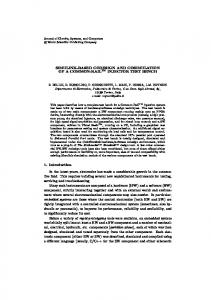


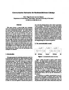


![[inria-00555890, v1] Computing the throughput of probabilistic ... - graal](https://m.moam.info/img/260x300/inria-00555890-v1-computing-the-throughput-of-prob_5ba7d8a5097c476b718b45a1.jpg)


