that is ideally zero when the filter nonlinearities are not excited. Next, in residue prediction, linear predictive codes are used to predict the nonzero .... sum based error detection and correction techniques in linear digital filters are presented in .... vector ui(t) and n-dimensional previous system states s(t) to generate the ...
Concurrent Error Detection in Nonlinear Digital Filters Using Checksum Linearization and Residue Prediction Suvadeep Banerjee* , Md Imran Momtaz* , and Abhijit Chatterjee* *
Georgia Institute of Technology
Abstract—Soft errors due to alpha particles, neutrons and environmental noise are of increasing concern due to aggressive technology scaling. While prior work has focused mostly on error resilience of linear signal processing algorithms, there is increasing need to address the same for nonlinear systems used in emerging applications for sensing and control. In this paper, a new approach for detecting errors in nonlinear digital filters is developed that does not require full duplication of all the nonlinear operations in the filter. First, a checksum of the linear least squares fit to the nonlinear function of the filter is derived that is ideally zero when the filter nonlinearities are not excited. Next, in residue prediction, linear predictive codes are used to predict the nonzero checksum error values that result exclusively from filter nonlinearity excitation. This allows fine granularity soft error detection at low hardware cost. Simulation experiments on a nonlinear Volterra filter prove the viability of the proposed concurrent error detection methodology.
I.
I NTRODUCTION
Aggressive technology scaling has led to considerable improvement in the performance of deep sub-micron high speed digital circuits. However, due to the increase in complexity of these circuits, they have become more susceptible to soft errors [1–3] which are caused by the impact of highly energetic particles such as alpha particles or neutrons on internal circuit nodes. These errors have become more dominant in scaled digital circuits due to feature-size reduction, almost near-doubling of operating frequency and supply voltage/threshold voltage scaling [4, 5]. With each technology generation, the node capacitance values further scale down, thus allowing soft errors to cause erroneous digital logic transitions at these nodes. Such intermittent and permanent failures are of particular concern in digital signal processing, control and communication applications. Lower supply voltage further increases the susceptibility of these circuits to external noise sources due to reduced noise margin. In systems with concurrently operating on-chip digital logic, analog/RF circuitry and mixed signal blocks such as data converters, noise can get coupled through the substrate as well as the power supply and ground planes, causing periodic logic upsets. Present architectural trends with shorter pipelines with reduced slack and higher clock rates make circuits more vulnerable to soft errors. Of increasing concern, in this context, are nonlinear digital filters that are extensively and routinely used in signal processing, communication and control applications where reliability and dependability are critical issues. In the past, significant research has been performed on methods for concurrent error
detection (CED) in linear digital circuits. Checksum codes for concurrent error detection and fault tolerance was first conceived and investigated by Jou and Abraham in [6]. This led to the research on algorithm-based fault tolerance (ABFT) which focused on highly concurrent structures widely used in signal processing algorithms such as matrix arithmetic and Fast Fourier Transform [7]. Real-number checksum codes were first developed and used in [8, 9] to perform error detection and correction in linear digital state variable systems. To resolve the high overhead required for error correction, probabilistic error compensation schemes were proposed in [10–13]. In safety-critical applications, traditional methods for error detection and correction rely on hardware duplication/triplication [14–17]. Error detection in non-linear systems generally involves partitioning of the circuit into linear and nonlinear components. Checksum codes are applied to the linear components for error detection whereas hardware and/or software redundancy is applied for error detection in the nonlinear modules. However, the high overhead in terms of power and area associated with these methods makes them relatively expensive in general applications. A more elegant error detection technique for non-linear systems was proposed in [18] based on time-freeze linearization which models a nonlinear digital filter using a time-varying linearized representation. The checksum circuit generates a time-varying checksum code for each single time frame by freezing the system dynamics between two adjacent time frames and linearizing the circuit behavior between the two frames. However, the method can result in duplication of all the nonlinear functions in the worst case and further requires that the wordlength precision of the checking circuitry be the same as that of the circuit under test (CUT). This incurs higher cost in terms of both complexity, area and power. In this paper, a low cost error detection technique for nonlinear digital filters using linearized checksum codes and linear predictive coding (LPC) algorithms is presented for the first time. First, a least squares linear fit to the nonlinear system is derived and checksum codes are applied to the derived best-fit linear model. When the circuit non-linearities are not excited by the input stimulus (such as for small-signal inputs), the checksum error is ideally zero. In the absence of soft errors, for large input signals, the checksum error carries the non-zero time-varying values which are proportional to the degree of circuit nonlinearity excitation by the stimulus applied. Linear predictive codes are applied to this time-varying error signal to detect soft errors using forward error prediction. The core
circuits [8]. A coding vector CV = [α1 , α2 , · · · , αn ] under the condition that each αi is real and non-zero, is applied on A, B, C, and D to encode the information of system dynamics such that X = CV.A and Y = CV.B. The checking circuit consists of a data checksum circuitry (DCC) and state checksum circuitry (SCC). The DCC computes the check variable from the next state as CV.s(t + 1) and the SCC does the same from the current state as c(t + 1) = Xs(t) + Yu(t). The final checksum error e(t + 1) is computed by subtracting the latter from the former. Under fault free conditions and in absence of any noise (either external or quantization noise), the outputs of the SCC and the DCC cancel each other and the error signal e(t + 1) is ideally zero. However, under faulty conditions, a non-zero value of error signal e(t + 1) will be generated which represents a transient or a permanent error in the system. Hence, the expression of checksum error e(t + 1) is given by,
contributions of this paper are: •
The proposed technique for nonlinear digital systems allows concurrent error detection with very high accuracy. In comparison with other error detection methods, the hardware overhead is relatively small due to the fact that the technique allows significant parts of the error detection circuit to be implemented using reduced precision arithmetic without compromising error coverage.
•
We further demonstrate that the proposed error detection scheme provides high coverage for both bit errors and word errors through simulation experiments on a nonlinear Volterra filter. The proposed technique is compared with time-freeze linearization method.
The rest of the paper is organized as follows. First, checksum based error detection and correction techniques in linear digital filters are presented in Section II. A brief overview of nonlinear digital circuits is summarized in Section III. This is followed by a short discussion of time-freeze linearization technique in Section IV. Section V introduces the proposed linearized checksum and residue prediction method. Finally, experimental results and conclusion are presented in Sections VI and VII. II.
e(t + 1) = CV.s(t + 1) − c(t + 1) III.
N ONLINEAR D IGITAL C IRCUITS : B RIEF D ISCUSSION
A generic data flow graph of a nonlinear digital circuit is indicated in Figure 1. The nonlinear state variable system implements a nonlinear transformation of the the elements of input vector u(t) and previous system states s(t). For example, a possible nonlinear function may be s(i)k or a product of integer powers of input elements. A general representation of a linear time-varying state-space system (a particular class of nonlinear systems) will be given as,
CED IN L INEAR D IGITAL C IRCUITS : R EVIEW
Linear time-invariant (LTI) systems, used extensively in control and signal processing applications, can be represented by linear state variable systems. The general representation of a linear state variable system consists of a computational block, which takes m primary inputs (u1 , u2 , · · · , um ) and current latched n system states (s1 , s2 , · · · sn ) to generate the system states for the next clock cycle as well as the l primary outputs (y1 , y2 , · · · , yl ). The computational block that we consider in this paper are interconnections of adders, multipliers, shifters, and registers. Given the state vector s(t) = [s1 (t), s2 (t), · · · , sn (t)]| , the input vector u(t) = [u1 (t), u2 (t), · · · , um (t)]| and output vector y(t) = [y1 (t), y2 (t), · · · , yl (t)]| at time t, a generalized representation of a linear system can be expressed by the following equations: s(t + 1) = As(t) + Bu(t) y(t + 1) = Cs(t) + Du(t)
(2)
s(t + 1) = A(t)s(t) + B(t)u(t) y(t + 1) = C(t)s(t) + D(t)u(t)
(3)
where all the matrices contain non-linear combinations of system states and inputs and are hence represented as timevarying. The usual method of implementing linear checksum in this system fails due to the constantly varying system matrices. This necessitates the development of nonlinear error detection techniques with reduced redundancy.
(1)
where matrices A, B, C and D are the system matrix, input matrix, output matrix and feedthrough matrix, respectively. Soft errors occur as bit flips either in the output of the computational blocks such as adders, multipliers, and shifters used in the system resulting in erroneous states(operator errors) or directly in the system states. In the former case, the error may propagate to the primary outputs or another system state. A system state error propagates through the digital logic structure to the primary outputs or to the other system states over multiple clock cycles. However, an error in the primary output does not propagate to other outputs or other states and disappears after one clock cycle. Hence, this paper primarily focuses on error detection in the system states only.
Fig. 1.
General structure of a nonlinear state variable system
IV.
T IME -F REEZE L INEARIZATION
The brute force method to concurrent error detection in nonlinear digital circuits is to duplicate and compare the outputs between the duplicate circuit and the circuit under test. This approach is expensive and introduces very high hardware overhead. To reduce the cost of error checking, one possible approach is time-freeze linearization [18]. In timefreeze linearization method, the nonlinear digital circuit is modeled as a linear digital circuit in each time frame by
Real number checksum codes has been proposed to be a powerful tool for concurrent error detection in linear digital 2
The nonlinear state space equation in (3) can be differently expressed as
freezing the values at circuit nodes corresponding to specified inputs of nonlinear circuit functions. The term freezing refers to treating the respective node values as constants over the width of a single time frame, even though these values change from one time frame to another. This facilitates the use of checksum codes, traditionally used in linear digital circuits for, concurrent error detection in non-linear digital circuits. The checking circuitry is economically designed, using tapped subfunctions from specific internal nodes of the non linear digital circuit. In a nonlinear system, the matrices A(t) and B(t) are constantly varying, thereby making the computation of matrices X and Y also time-varying in the state checksum circuitry (SCC). Time-freeze linearization allows one to design the SCC in a way such that at each time instant the matrices X and Y are computed by using tapped subfunctions of system states. Although, this approach is followed to reduce error detection cost by avoiding hardware and/or software redundancy, this complicates the design of the checksum circuitry. This necessitates more investigation for a simpler solution which will be able to perform concurrent error detection in nonlinear digital systems at further reduced cost. V.
s(t + 1) = M(t)z(t)
(4) |
|
where M(t) = [A B] and z(t) = [s(t) u(t) ]. Now, the linear least squares problem is posed as: Given b sets of input-output pairs pj and qj , ∀1 ≤ j ≤ ˆ a linear estimate of M, such that with the b, determine M, Pb ˆ ˆ = Mp, linear estimate q the total error j=1 ||ˆ qj − qj ||2 is ˆ is determined, it can be decomposed to minimized. Once M ˆ and B, ˆ the linear estimates of the system matrix A obtain A ˆ is given and the input matrix B. The algorithm to obtain M as, Algorithm 1:
1: 2:
L INEARIZED C HECKSUM AND R ESIDUE P REDICTION
3: 4: 5: 6: 7:
The basic idea of the proposed approach is to separate the linear and nonlinear dynamics of the system. It has been mentioned in Section II that under fault-free conditions, the checksum error is ideally zero. However, if a checksum error signal for a nonlinear system is generated based on a leastsquares linear estimate of the same system, it will be non-zero even under fault free conditions, since there will be estimation mismatch between linear and nonlinear system dynamics. This non-zero error, in fact, stems solely from the excitation of nonlinearities in the circuit. A prediction mechanism predicts the next checksum value based on a history of past error samples. In presence of fault(s) in the system, the predictor cannot predict the irregularity experienced on the checksum error signal. Thus, the diagnosis is performed by continually comparing the predictor output and the actual linearized checksum circuit output and the residue between the two signals is the actual error signal.
Create matrix H = [p1 , p2 , · · · , pb ]| . Perform Singular Value Decomposition (SVD) of H = UΣV∗ . Create Moore-Penrose Pseudo-Inverse G = VΣ−1 U∗ . for j = 1 : n do Create vector d = [q1 (j), q2 (j), · · · , qb (j)]| . ˆ as G.d. Generate jth row of M end for
ˆ is determined, A ˆ and B ˆ are separated out blockOnce M wise in the same manner as M is formed. The proposed approach is depicted in the block diagram of Figure 2. One of the primary advantages of the proposed approach is that the least squares computation is a one-time design stage procedure to determine the linearized checksum. Hence, this saves considerable amount of computational overhead in comparison to time-freeze linearization where some of the nonlinear functions need to be replicated in hardware.
A. Linearized Checksum Generation
Fig. 2.
The least squares linear estimate of a nonlinear system involves the generation of sufficient number of training pair of input-output samples. Let us consider the general nonlinear system of equation (3). We apply r different sets of input vectors u1 (t), u2 (t), · · · , ur (t) to the nonlinear system, one at a time. For each input vector ui , ∀1 ≤ i ≤ r, the nonlinear system is simulated for a fixed number of samples, say k samples starting from an initial system state. At each sampling time instant, the input to the system are m-dimensional input vector ui (t) and n-dimensional previous system states s(t) to generate the n-dimensional new system states s(t + 1). This can be perceived as a system with (n + m)-dimensional input vector p(t) = [sui (t)| ui (t)| ] and n-dimensional output vector q(t) = sui (t + 1) where the subscript ui denotes the system state with input ui . Hence, for each input vector ui , k pairs of input-output samples p and q are generated. Across r different sets of input vectors, a total of r x k = b (say) pairs of input-output samples are generated.
Block Diagram of the Linear Estimation Method
The selection of input vectors ui , ∀1 ≤ i ≤ r needs to be made carefully. For generation of training samples, the input vectors should be chosen from an input set which are expected to be applied to the nonlinear system during actual deployment. The least squares linear estimate of the system changes with the choice of input vectors. The reason for this behavior can be explained by the fact that different input vectors excite the nonlinearities of the system in different ways. A least squares estimate tries to fit a linear state-space trajectory of the system to the actual nonlinear trajectory that the circuit goes through. Depending on the choice of input vector, specific nonlinearities of the circuit can be activated and the nonlinear trajectory will be different. The choice of number of input vectors is guided by the tradeoff between nonlinearity coverage and linear overfitting. A very small set of input vectors will be insufficient to excite all nonlinearities and create an accurate linear estimate of the system while a large set of input vectors 3
requires higher computational resources and may result in linear model overfitting. The same tradeoff dictates the choice of k - the number of samples generated from simulation with each input vector.
the predicted checksum and the actual checksum will again be non-zero due to prediction mismatch of the predictor. This prediction mismatch is controlled by the filter order of the LPC predictor and the sample history considered. However, in fault-free conditions, this prediction mismatch lies within a distinct threshold. In presence of fault(s) in the system, the actual checksum error shows a distinct discrepancy from the usual trend at the instant of fault occurrence and the predictor is unable to predict this unusual signal behavior from its past history. Therefore, the difference between two signals is higher than the chosen threshold in absolute magnitude and the fault is detected. Depending on the predictor parameters (filter taps and signal history length), the threshold changes. A higher filter order and longer signal history will lower the threshold by reducing prediction mismatch and improve performance at the cost of resource overhead.
ˆ and B ˆ are determined, the linear checksum module Once A ˆ = CV.A ˆ and computes a linear checksum by selecting X ˆ ˆ Y = CV.B. Hence, in this case, the SCC computes cˆ(t+1) = ˆ ˆ Xs(t) + Yu(t) and generates the checksum error signal by subtracting this check signal from the usual output of DCC: CV.s(t + 1). Unlike linear case, the difference between SCC and DCC outputs will not be zero since the SCC computation is based on the linear estimate of the system. This nonzero error signal is fed into the linear predictive coding (LPC) unit for further processing. B. Residue Prediction
It can be argued that linear predictive codes can directly be applied to the sum of all the states of a digital system to remove the computational cost of system linearization. Under error-free conditions, the sum of system states follows a definite trajectory which can similarly be predicted by LPC. In presence of errors, the sum of the states deviate from the usual trend and the predictor residue will detect the error. However, this scheme will suffer from practical drawbacks. The sum of system states results in very large dynamic range of signals and hence the checking circuit needs to have higher dynamic range adding to the hardware resource cost. On the other hand, the predictor residue in our proposed approach has a small value which can be resolved using circuits with lower precision.
Linear predictive coding (LPC) is a powerful predictive tool widely used in digital signal processing domain, mostly in speech and audio signal processing [19–22]. It denotes a mathematical operation where future values of a discrete-time signal are estimated as a linear function of previous samples. The most general representation is, given a discrete-time signal x with (n − 1) samples, the prediction for the nth sample is, x ˆ(n) =
p X
ai x(n − i)
(5)
i=1
where x ˆ(n) is the predicted signal, x(n − i) the previous samples of the signal and ai the coefficients of the predictor (FIR filter). The sample history used for the prediction is controlled by the parameter p. The objective is to minimize the estimate error �(n) = x ˆ(n) − x(n). This problem is wellstudied in the field of linear algebra where the most common choice in optimization of parameters ai is to solve the YuleWalker autocorrelation (AR) equations derived by minimizing the expected value of the squared error E[�2 (n)]. We use the well known Levinson-Durbin recursion method [23] to solve the Yule Walker equations.
VI.
S IMULATION R ESULTS
We perform simulation experiments on a nonlinear Volterra filter consisting of 13 multipliers and 10 adders whose statespace representation is given by equation (6) [18], in MATLAB environment. s1 (t + 1) s2 (t + 1) s (t + 1) = 3 s4 (t + 1) 0 0 0 0 0 0 0 1 0.183 −0.946 F + 0.197 F − 0.241 02 12 0 0 1 0
Fig. 3. Block Diagram of Linearized Checksum and Residue Prediction Methodology
In our case, the linearized checksum error signal e is fed to the LPC unit as shown in Figure 3. The LPC unit solves the Yule-Walker AR equations to obtain the FIR filter coefficients which are then used to predict the next checksum error signal eˆ. The actual checksum error signal in the next instant is compared with the predicted checksum error signal through a comparator and the difference between the two is referred to as predictor residue. This residue signal is used for error detection. In a fault-free system, the linearized checksum signal e is non-zero due to the mismatch between actual nonlinear system dynamics and linear estimation. Now, this non-zero error signal is predicted through LPC in successive time instants using past values of the checksum error. The difference between
s1 (t) 1 s (t) 0 2 s3 (t) 0.1 s (t) 4 0 u(t) (6)
where F02 (t) = −0.971s1 (t) + 0.946s2 (t) + 0.552u(t) and F12 (t) = 0.183s1 (t)+0.072s2 (t)+0.298u(t). Thus the system matrix of this filter contains polynomial functions of the states and input signal and continuously varies over time. One of the primary uses of a Volterra filter is in the field of digital telecommunication where it is used as a predistorter to compensate for intermodulation distortion in devices like power amplifiers and frequency mixers. Hence, in our experiments we applied orthogonal frequency-division multiplexing (OFDM) signals as input u(t) to the system. We chose 64-QAM modulation scheme with a carrier frequency of 1 GHz to generate an OFDM input signal. We chose a total 4
of r = 4 different digital bit sequences to generate different OFDM stimuli which are then used as inputs to the Volterra filter of (6) to generate the data pair p and q. The simulation with each input is performed over 1000 time samples. Using these data, we generate the least-squares linear fit to the system in (6) by the SVD linearization method mentioned in Section V. The linear estimate of the system is obtained as, 0 ˆ = 1 M 0.1824 0
0 0 −0.9158 0
0 0 0.2062 1
0 0 −0.3389 0
and the DCC operate on the same data at next instant t + 1 which is simply evident from checksum definition in Section II. However, in a nonlinear time-varying system, the effects of an injected soft error take a few clock cycles to decay and determined by the effective time-constant of the excited nonlinearities. We determined this time-constant to be 15 cycles in our simulation setup under the mentioned conditions. Hence, both bit errors and word errors are injected every 15 clock cycles. The number of least significant bits affected during an error injection is referred to as the injection range. We conducted experiments in which bit errors are injected into all W bits of a data word, and then into only the least significant W W W 2 , 4 and 8 bits, respectively. The same experiments are also run using time-freeze linearization method. The results of our experiment with different word sizes for both bit errors and word errors are shown in Figures 4 and 5.
1 0 0.1086 0 (7)
We use this matrix to compute the linearized checksum signal of SCC. The nominal coding vector chosen in this simulation is CV = [0.25 0.25 0.25 0.25]. Pn It is useful to select CV in a way such that the constraint i=1 |CV(i)| ≤ 1 is satisfied to avoid overflow errors [9]. However, it should be mentioned that fault coverage changes with the choice of coding vector which we demonstrate later. The optimal choice of coding vector is a topic of future research and is beyond the scope of this paper. For fault injection, we study two kinds of faults: those that cause single data bits of state output data word to be different from their correct values and those that cause multiple data bits to be incorrect. The first is commonly referred as a bit error and the latter is called a word error. We discretize each output state with a word size of W bits with 1 bit reserved for signed number representation. Among the (W − 1) bits, W 2 bits are used to represent the decimal portion of the number. Bit errors are injected into the system by selecting a state at random (with equal probability) and then by complementing any one bit chosen at random where each bit has equal probability of being complemented. Similarly, word errors are injected by either complementing or not complementing each bit of the data word randomly selected from the n states, the probability of bit complementation being 0.5. A nominal fault-free simulation is performed using the linearized checksum. The predictor selected for our simulation has a filter order of 4 and uses a past history of 8 samples. As mentioned in Section V, an error is detected only if the difference between LPC predictor output and the linearized checksum signal is above a fixed threshold. This threshold is due to three main reasons: 1) Estimate mismatch between actual nonlinear dynamics and linearized checksum, 2) Prediction mismatch between LPC predictor and the checksum error signal, and 3) Quantization noise due to finite precision arithmetic. From nominal simulations, the linearized checksum signal is seen to be less than 0.05 in magnitude without any injected errors and hence this threshold level of 0.05 was chosen to be the error detection threshold during actual error injection. If a different nonlinear system is considered, this threshold will be different and needs to be determined from nominal fault-free simulations.
Fig. 4.
Fault Coverage vs Injection Range for Bit Errors
Fig. 5.
Fault Coverage vs Injection Range for Word Errors
In figures 4 and 5, a lower value of ratio between injection range and data word length indicates error injection in LSBs whereas a higher value indicates error injection in bits of higher significance. From the results, it is clearly seen that bit errors in the least significant bits are harder to detect in both the proposed approach and time-freeze linearization. However, we demonstrate that our proposed approach is superior in detection of bit errors whereas it performs on a similar scale for word errors. Since word errors, in general, have multiple bit errors, these are easier to detect than bit errors. The coverage increases as the word length is increased since it allows better resolution for faults to get detected. The predictor residue signal in the nominal system and with single error injection are shown in Figure 6. The low value of the signal allows us to use checking circuit with reduced precision and we use a precision of W/2 bits for a word length of W bits.
In a linear time-invariant system, errors can be injected every alternate time frame, since the errors do not accumulate over time as far as linear check variables are concerned. Though finite precision arithmetic errors and injected soft errors accumulate between times t and t + 1, both the SCC
Table I indicates the variation of error coverage with different choices of coding vectors with a word length of 8 5
[3]
[4]
[5]
[6] Fig. 6.
Comparison of Predictor Residue without and with Error Injection [7]
bits. The results clearly show that future research is needed to optimize the choice of coding vector. Different sets of coding vectors control the sensitivity of the contribution of system states to the checksum error line. TABLE I.
bit bits bits bits
[9]
E RROR C OVERAGE WITH DIFFERENT C ODING V ECTORS
Injection Range 1 2 4 8
[8]
Bit Error CV1 0.0166 0.05 0.44 0.57
Coverage CV2 0.0182 0.0524 0.32 0.62
[10]
Word Error Coverage CV1 CV2 0.0082 0.0155 0.0421 0.0791 0.7015 0.68 0.8566 0.79
[11]
where the 2 coding vectors CV1 and CV2 are given as, CV1 = [0.25 0.25 0.25 0.25] and CV2 = [0.15 0.15 -0.4 0.25]. VII.
[12]
C ONCLUSION [13]
Soft errors are becoming an issue of increasing concern in nonlinear digital circuits frequently encountered in sensing, control and communication applications. In this paper we have described a new methodology for detection of soft errors in nonlinear digital state variable systems. The proposed technique generates a least-squares linear fit to the nonlinear system with the aid of singular value decomposition (SVD). Linearized checksum codes are derived from the linear system estimate which are then used to predict the error signal using linear predictive codes. We demonstrate that the predictor residue signal can be used for fine-grained error detection through a simulation of a nonlinear digital Volterra filter. We have further shown that our methodology outperforms time-freeze linearization in terms of error detection capability at reduced overhead, since the latter needs duplication of the system in the worst case. The experimental analysis has been performed for both single bit errors and multiple bit word errors. The results indicate the viability of the proposed technique and provides direction for further research.
[14] [15]
[16]
[17]
[18]
[19]
[20]
ACKNOWLEDGMENTS We acknowledge support for this research from NSF Grant CISE: CCF:1421353.
[21]
R EFERENCES [22]
[1]
P. Shivakumar, M. Kistler, S. Keckler, D. Burger, and L. Alvisi, “Modeling the effect of technology trends on the soft error rate of combinational logic,” in Dependable Systems and Networks, 2002. DSN 2002. Proceedings. International Conference on, 2002, pp. 389–398. [2] R. Iyer, N. Nakka, Z. Kalbarczyk, and S. Mitra, “Recent advances and new avenues in hardware-level reliability support,” Micro, IEEE, vol. 25, no. 6, pp. 18–29, Nov 2005.
[23]
6
T. Karnik, B. Bloechel, K. Soumyanath, V. De, and S. Borkar, “Scaling trends of cosmic ray induced soft errors in static latches beyond 0.18 /spl mu/,” in VLSI Circuits, 2001. Digest of Technical Papers. 2001 Symposium on, June 2001, pp. 61–62. B. Shim and N. Shanbhag, “Reduced precision redundancy for lowpower digital filtering,” in Signals, Systems and Computers, 2001. Conference Record of the Thirty-Fifth Asilomar Conference on, vol. 1, Nov 2001, pp. 148–152 vol.1. Y. Dhillon, A. Diril, and A. Chatterjee, “Soft-error tolerance analysis and optimization of nanometer circuits,” in Design, Automation and Test in Europe, 2005. Proceedings, March 2005, pp. 288–293 Vol. 1. J.-Y. Jou and J. Abraham, “Fault-tolerant matrix arithmetic and signal processing on highly concurrent computing structures,” Proceedings of the IEEE, vol. 74, no. 5, pp. 732–741, May 1986. J.-Y. Jou and J. Abraham, “Fault-tolerant FFT networks,” Computers, IEEE Transactions on, vol. 37, no. 5, pp. 548–561, May 1988. V. Nair and J. Abraham, “Real-number codes for fault-tolerant matrix operations on processor arrays,” Computers, IEEE Transactions on, vol. 39, no. 4, pp. 426–435, Apr 1990. A. Chatterjee and M. d’Abreu, “The design of fault-tolerant linear digital state variable systems: theory and techniques,” Computers, IEEE Transactions on, vol. 42, no. 7, pp. 794–808, Jul 1993. M. Ashouei and A. Chatterjee, “Checksum-based probabilistic transienterror compensation for linear digital systems,” Very Large Scale Integration (VLSI) Systems, IEEE Transactions on, vol. 17, no. 10, pp. 1447–1460, Oct 2009. M. Nisar and A. Chatterjee, “Guided probabilistic checksums for error control in low power digital-filters,” in On-Line Testing Symposium, 2008. IOLTS ’08. 14th IEEE International, July 2008, pp. 239–244. M. Ashouei, S. Bhattacharya, and A. Chatterjee, “Design of soft error resilient linear digital filters using checksum-based probabilistic error correction,” in VLSI Test Symposium, 2006. Proceedings. 24th IEEE, April 2006, pp. 6 pp.–213. M. Ashouei, S. Bhattacharya, and A. Chatterjee, “Improving SNR for DSM linear systems using probabilistic error correction and state restoration: A comparative study,” in Test Symposium, 2006. ETS ’06. Eleventh IEEE European, May 2006, pp. 35–42. B. Johnson, Design and Analysis of Fault Tolerant Digital System. Addison-Wesley, 1989. N. Shanbhag, “Reliable and energy-efficient digital signal processing,” in Design Automation Conference, 2002. Proceedings. 39th, 2002, pp. 830–835. R. Hegde and N. Shanbhag, “Soft digital signal processing,” Very Large Scale Integration (VLSI) Systems, IEEE Transactions on, vol. 9, no. 6, pp. 813–823, Dec 2001. B. Shim and N. Shanbhag, “Energy-efficient soft error-tolerant digital signal processing,” Very Large Scale Integration (VLSI) Systems, IEEE Transactions on, vol. 14, no. 4, pp. 336–348, April 2006. A. Chatterjee and R. Roy, “Concurrent error detection in nonlinear digital circuits using time-freeze linearization,” Computers, IEEE Transactions on, vol. 46, no. 11, pp. 1208–1218, Nov 1997. Y. Tang, T. Li, and C. Suen, “VLSI arrays for speech processing with linear predictive coding,” in Pattern Recognition, 1994. Vol. 3 - Conference C: Signal Processing, Proceedings of the 12th IAPR International Conference on, Oct 1994, pp. 357–359 vol.3. A. Harma and U. Laine, “A comparison of warped and conventional linear predictive coding,” Speech and Audio Processing, IEEE Transactions on, vol. 9, no. 5, pp. 579–588, Jul 2001. R. Hendriks, R. Heusdens, and J. Jensen, “Perceptual linear predictive noise modelling for sinusoid-plus-noise audio coding,” in Acoustics, Speech, and Signal Processing, 2004. Proceedings. (ICASSP ’04). IEEE International Conference on, vol. 4, May 2004, pp. iv–189–iv–192 vol.4. W. Kinsner and E. Vera, “Fractal modelling of residues in linear predictive coding of speech,” in Cognitive Informatics, 2009. ICCI ’09. 8th IEEE International Conference on, June 2009, pp. 181–187. N. Levinson, “The Wiener RMS (root mean square) error criterion in filter design and prediction.”