Apr 29, 2011 - [2] identified a set of consistency desiderata for dynamic map labeling. .... Figure 2 shows all eight boundary intersection events. Each of the.
Consistent Labeling of Rotating Maps Andreas Gemsa? , Martin N¨ollenburg? , Ignaz Rutter
arXiv:1104.5634v1 [cs.CG] 29 Apr 2011
Institute of Theoretical Informatics, Karlsruhe Institute of Technology (KIT), Germany
Abstract. Dynamic maps that allow continuous map rotations, e.g., on mobile devices, encounter new issues unseen in static map labeling before. We study the following dynamic map labeling problem: The input is a static, labeled map, i.e., a set P of points in the plane with attached nonoverlapping horizontal rectangular labels. The goal is to find a consistent labeling of P under rotation that maximizes the number of visible labels for all rotation angles such that the labels remain horizontal while the map is rotated. A labeling is consistent if a single active interval of angles is selected for each label such that labels neither intersect each other nor occlude points in P at any rotation angle. We first introduce a general model for labeling rotating maps and derive basic geometric properties of consistent solutions. We show NPcompleteness of the active interval maximization problem even for unitsquare labels. We then present a constant-factor approximation for this problem based on line stabbing, and refine it further into an efficient polynomial-time approximation scheme (EPTAS). Finally, we extend the EPTAS to the more general setting of rectangular labels of bounded size and aspect ratio.
1
Introduction
Dynamic maps, in which the user can navigate continuously through space, are becoming increasingly important in scientific and commercial GIS applications as well as in personal mapping applications. In particular GPS-equipped mobile devices offer various new possibilities for interactive, location-aware maps. A common principle in dynamic maps is that users can pan, rotate, and zoom the map view. Despite the popularity of several commercial and free applications, relatively little attention has been paid to provably good labeling algorithms for dynamic maps. Been et al. [2] identified a set of consistency desiderata for dynamic map labeling. Labels should neither “jump” (suddenly change position or size) nor “pop” (appear and disappear more than once) during monotonous map navigation; moreover, the labeling should be a function of the selected map viewport and not depend on the user’s navigation history. Previous work on the topic has focused solely on supporting zooming and/or panning of the map [2, 3, 11], ?
Supported by the Concept for the Future of KIT within the framework of the German Excellence Initiative.
2
Andreas Gemsa, Martin N¨ ollenburg, Ignaz Rutter
(a)
(b) Label 5 Label 4 Label 3 Label 2 Label 1
(c) 4 Label Label 5 Label 3 2 Label Label 1
(d) Label 4
Label 1
Label 5Label 2 Label 3
Label 1 Label 2 Label 4 Label 3 Label 5
Fig. 1: Input map with five points (a) and three rotated views with some partially occluded labels (b)–(d). whereas consistent labeling under map rotations has not been considered prior to this paper. Most maps come with a natural orientation (usually the northern direction facing upward), but applications such as car or pedestrian navigation often rotate the map view dynamically to be always forward facing [5]. Still, the labels must remain horizontally aligned for best readability regardless of the actual rotation angle of the map. A basic requirement in static and dynamic label placement is that labels are pairwise disjoint, i.e., in general not all labels can be placed simultaneously. For labeling point features, it is further required that each label, usually modeled as a rectangle, touches the labeled point on its boundary. It is often not allowed that labels occlude the input point of another label. Figure 1 shows an example of a map that is rotated and labeled. The objective in map labeling is usually to place as many labels as possible. Translating this into the context of rotating maps means that, integrated over one full rotation from 0 to 2π, we want to maximize the number of visible labels. The consistency requirements of Been et al. [2] can immediately be applied for rotating maps. Our Results. Initially, we define a model for rotating maps and show some basic properties of the different types of conflicts that may arise during rotation. Next, we prove that consistently labeling rotating maps is NP-complete, for the maximization of the total number of visible labels in one full rotation and NPhard for the maximization of the visibility range of the least visible label. Finally, we present a new 1/4-approximation algorithm and an efficient polynomial-time approximation scheme (EPTAS) for unit-height rectangles. A PTAS is called efficient if its running time is O(f (ε)·poly(n)). Both algorithms can be extended to the case of rectangular labels with the property that the ratio of the smallest and largest width, the ratio of the smallest and largest height, as well as the aspect ratio of every label is bounded by a constant, even if we allow the anchor point of each label to be an arbitrary point of the label. This applies to most practical scenarios where labels typically consist of few and relatively short lines of text. Related Work. Most previous algorithmic research efforts on automated label placement cover static labeling models for point, line, or area features. For static point labeling, fixed-position models and slider models have been introduced [4, 8], in which the label, represented by its bounding box, needs to touch the labeled
Consistent Labeling of Rotating Maps
3
point along its boundary. The label number maximization problem is NP-hard even for the simplest labeling models, whereas there are efficient algorithms for the decision problem that asks whether all points can be labeled in some of the simpler models (see the discussion by Klau and Mutzel [7] or the comprehensive map labeling bibliography [14]). Approximation results [1,8], heuristics [13], and exact approaches [7] are known for many variants of the static label number maximization problem. In recent years, dynamic map labeling has emerged as a new research topic that gives rise to many unsolved algorithmic problems. Petzold et al. [12] used a preprocessing step to generate a reactive conflict graph that represents possible label overlaps for maps of all scales. For any fixed scale and map region, their method computes a conflict-free labeling using heuristics. Mote [10] presents another fast heuristic method for dynamic conflict resolution in label placement that does not require preprocessing. The consistency desiderata of Been et al. [2] for dynamic labeling (no popping and jumping effects when panning and zooming), however, are not satisfied by either of the methods. Been et al. [3] showed NP-hardness of the label number maximization problem in the consistent labeling model and presented several approximation algorithms for the problem. N¨ ollenburg et al. [11] recently studied a dynamic version of the alternative boundary labeling model, in which labels are placed at the sides of the map and connected to their points by leaders. They presented an algorithm to precompute a data structure that represents an optimal one-sided labeling for all possible scales and thus allows continuous zooming and panning. None of the existing dynamic map labeling approaches supports map rotation.
2
Model
In this section we describe a general model for rotating maps with axis-aligned rectangular labels. Let M be a labeled input map, i.e., a set P = {p1 , . . . , pn } of points in the plane together with a set L = {`1 , . . . , `n } of pairwise disjoint, closed, and axis-aligned rectangular labels, where each point pi is a point on the boundary ∂`i of its label `i . We say `i is anchored at pi . As M is rotated, each label `i in L remains horizontally aligned and anchored at pi . Thus, label intersections form and disappear during rotation of M . We take the following alternative perspective on the rotation of M . Rather than rotating the points, say clockwise, and keeping labels horizontal we may instead rotate each label around its anchor point counterclockwise and keep the set of points fixed. It is easy to see that both rotations are equivalent and yield exactly the same results. A rotation of L is defined by a rotation angle α ∈ [0, 2π); a rotation labeling of M is a function φ : L×[0, 2π) → {0, 1} such that φ(`, α) = 1 if label ` is visible or active in the rotation of L by α, and φ(`, α) = 0 otherwise. We call a labeling φ valid if, for any rotation α, the set of labels L(α) = {` ∈ L | φ(`, α) = 1} consists of pairwise disjoint labels and no label in L(α) contains any point in P (other than its anchor point). We note that a valid labeling is not yet consistent in terms of the definition of Been et al. [2, 3]: given fixed anchor points, labels
4
Andreas Gemsa, Martin N¨ ollenburg, Ignaz Rutter
clearly do not jump and the labeling is independent of the rotation history, but labels may still pop during a full rotation from 0 to 2π, i.e., appear and disappear more than once. In order to avoid popping effects, each label may be active only in a single contiguous range of [0, 2π), where ranges are circular ranges modulo 2π so that they may span the input rotation α = 0. A valid labeling φ, in which for every label ` the set Aφ (`) = {α ∈ [0, 2π) | φ(`, α) = 1} is a contiguous range modulo 2π, is called a consistent labeling. For a consistent labeling φ the set Aφ (`) is called the active range of `. The length |Aφ (`)| of an active range Aφ (`) is defined as the length of the circular arc {(cos α, sin α) | α ∈ Aφ (`)} on the unit circle. The objective in static map labeling is usually to find a maximum subset of pairwise disjoint labels, i.e., to label as many points as possible. Generalizing this objective to rotating maps means that integrated over all rotations α ∈ [0, 2π) we wantP to display as many labels as possible. This corresponds to maximizing the sum `∈L |Aφ (`)| over all consistent labelings φ of M ; we call this optimization problem MaxTotal. An alternative objective is to maximize over all consistent labelings φ the minimum length min` |Aφ (`)| of all active ranges; this problem is called MaxMin.
3
Properties of consistent labelings
In this section we show basic properties of consistent labelings. If two labels ` and `0 intersect in a rotation of α they have a (regular) conflict at α, i.e., in a consistent labeling at most one of them can be active at α. The set C(`, `0 ) = {α ∈ [0, 2π) | ` and `0 are in conflict at α} is called the conflict set of ` and `0 . We show the following lemma in a more general model, in which the anchor point p of a label ` can be any point within ` and not necessarily a point on the boundary ∂`. Lemma 1. For any two labels ` and `0 with anchor points p ∈ ` and p0 ∈ `0 the set C(`, `0 ) consists of at most four disjoint contiguous conflict ranges. Proof. The first observation is that due to the simultaneous rotation of all initially axis-parallel labels in L, ` and `0 remain “parallel” at any rotation angle α. Rotation is a continuous movement and hence any maximal contiguous conflict range in C(`, `0 ) must be a closed “interval” [α, β], where 0 ≤ α, β < 2π. Here we explicitly allow α > β by defining, in that case, [α, β] = [α, 2π) ∪ [0, β]. At a rotation of α (resp. β) the two labels ` and `0 intersect only on their boundary. Let l, r, t, b be the left, right, top, and bottom sides of ` and let l0 , r0 , t0 , b0 be the left, right, top, and bottom sides of `0 (defined at a rotation of 0). Since ` and `0 are parallel, the only possible cases, in which they intersect on their boundary but not in their interior are t ∩ b0 , b ∩ t0 , l ∩ r0 , and r ∩ l0 . Each of those four cases may appear twice, once for each pair of opposite corners contained in the intersection. Figure 2 shows all eight boundary intersection events. Each of the conflicts defines a unique rotation angle and obviously at most four disjoint conflict ranges can be defined with these eight rotation angles as their endpoints. t u
Consistent Labeling of Rotating Maps
t0
t
r l0 `0
` l
b
r b0
t
b
b0
0 l r `0
(d) l ∩ r
r
l0
t0
l ` t
`
0
(e) l ∩ r
t
l
0
`
` b
r
b
0
b0 l0
l t0 (c) b ∩ t0
b l0
`0
l `
r
t0
t
0
t0
l0
`0
t
b0
r0
r0
b
(b) b ∩ t0
b `
r
b0
l0
b
l
r0
`0
`
(a) r ∩ l0
r
t0
r
t
0
5
r0
(f) t ∩ b
t
l `
r0 b
(g) t ∩ b0
l0 r b0
b0 `0
l0 t0
0
t0 0
`
r0
(h) r ∩ l0
Fig. 2: Two labels ` and `0 and their eight possible boundary intersection events. Anchor points are marked as black dots. t l wl
ht
wr
p
hb
r `
b Fig. 3: Parameters of label ` anchored at p.
In the following we look more closely at the conditions under which the boundary intersection events (also called conflict events) occur and at the rotation angles defining them. Let ht and hb be the distances from p to t and b, respectively. Similarly, let wl and wb be the distances from p to l and r, respectively (see Figure 3). By h0t , h0b , wl0 , and wr0 we denote the corresponding values for label `0 . Finally, let d be the distance of the two anchor points p and p0 . To improve readability of the following lemmas we define two functions fd (x) = arcsin(x/d) and gd (x) = arccos(x/d). Lemma 2. Let ` and `0 be two labels anchored at points p and p0 . Then the conflict events in C(`, `0 ) are a subset of C = {2π − fd (ht + h0b ), π + fd (ht + h0b ), fd (hb + h0t ), π − fd (hb + h0t ), 2π − gd (wr + wl0 ), gd (wr + wl0 ), π − gd (wl + wr0 ), π + gd (wl + wr0 )}. Proof. Assume without loss of generality that p and p0 lie on a horizontal line. First we show that the possible conflict events are precisely the rotation angles
6
Andreas Gemsa, Martin N¨ ollenburg, Ignaz Rutter
p
t α
p0 `0
d
`
b0
` ht +
b0
p
d α
t
h0b
ht +
(a) rotation of 2π − α
p0
`0 h0b
(b) rotation of π + α
Fig. 4: Boundary intersection events for t ∩ b0 .
p `
β
wr + wl0
d
l0
p0
r
(a) rotation of 2π − β
0
`
wr + wl0
r p0
p `
β
d
`0
l0
(b) rotation of β
Fig. 5: Boundary intersection events for r ∩ l0 .
in C. We start considering the intersection of the two sides t and b0 . If there is a rotation angle under which t and b0 intersect then we have the situation depicted in Figure 4 and by simple trigonometric reasoning the two rotation angles at which the conflict events occur are 2π − arcsin((ht + h0b )/d) and π + arcsin((ht + h0b )/d). Obviously, we need d ≥ ht + h0b . Furthermore, for the intersection in Figure 4a to be non-empty, we need d2 ≤ (wr + wl0 )2 + (ht + h0b )2 ; similarly, for the intersection in Figure 4b, we need d2 ≤ (wl + wr0 )2 + (ht + h0b )2 . From an analogous argument we obtain that the rotation angles under which b and t0 intersect are arcsin((hb + h0t )/d) and π − arcsin((hb + h0t )/d). Clearly, we need d ≥ hb + h0t . Furthermore, we need d2 ≤ (wr + wl0 )2 + (hb + h0t )2 for the first intersection and d2 ≤ (wl + wr0 )2 + (hb + h0t )2 for the second intersection to be non-empty under the above rotations. The next case is the intersection of the two sides r and l0 , depicted in Figure 5. Here the two rotation angles at which the conflict events occur are 2π − arccos((wr + wl0 )/d) and arccos((wr + wl0 )/d). For the first conflict event we need d2 ≤ (wr + wl0 )2 + (ht + h0b )2 , and for the second we need d2 ≤ (wr + wl0 )2 + (hb + h0t )2 . For each of the intersections to be non-empty we additionally require that d ≥ wr + wl0 . Similar reasoning for the final conflict events of l∩r0 yields the rotation angles π − arccos((wl + wr0 )/d) and π + arccos((wl + wr0 )/d). The additional constraints are d ≥ wl + wr0 for both events and d2 ≤ (wl + wr0 )2 + (hb + h0t )2 for the first intersection and d2 ≤ (wl +wr0 )2 +(ht +h0b )2 . Thus, C contains all possible conflict events. t u
Consistent Labeling of Rotating Maps
7
hard conflict range
p `
p0
`0
Fig. 6: Conflict ranges of two labels ` and `0 marked in bold on the enclosing circles.
One of the requirements for a valid labeling is that no label may contain a point in P other than its anchor point. For each label ` this gives rise to a special class of conflict ranges, called hard conflict ranges, in which ` may never be active. The rotation angles at which hard conflicts start or end are called hard conflict events. Every angle that is a (hard) conflict event is called a label event. Obviously, every hard conflict is also a regular conflict. Regular conflicts that are not hard conflicts are also called soft conflicts. We note that by definition regular conflicts are symmetric, i.e., C(`, `0 ) = C(`0 , `), whereas hard conflicts are not symmetric. The next lemma characterizes the hard conflict ranges. Lemma 3. For a label ` anchored at point p and a point q 6= p in P , the hard conflict events of ` and q are a subset of H = {2π − fd (ht ), π + fd (ht ), fd (hb ), π − fd (hb ), 2π − gd (wr ), gd (wr ), π − gd (wl ), π + gd (wl )}. Proof. We define a label of width and height 0 for q, i.e., we set h0t = h0b = wl0 = t u wr0 = 0. Then the result follows immediately from Lemma 2. A simple way to visualize conflict ranges and hard conflict ranges is to mark, for each label ` anchored at p and each of its (hard) conflict ranges, the circular arcs on the circle centered at p and enclosing `. Figure 6 shows an example. In the following we show that the MaxTotal problem can be discretized in the sense that there exists an optimal solution whose active ranges are defined as intervals whose borders are label events. An active range border of a label ` is an angle α that is characterized by the property that the labeling φ is not constant in any ε-neighborhood of α. We call an active range where both borders are label events a regular active range. Lemma 4. Given a labeled map M there is an optimal rotation labeling of M consisting of only regular active ranges. Proof. Let φ be an optimal labeling with a minimum number of active range borders that are no label events. Assume that there is at least one active range border β that is no label event. Let α and γ be the two adjacent active range borders of β, i.e., α < β < γ, where α and γ are active range borders, but not
8
Andreas Gemsa, Martin N¨ ollenburg, Ignaz Rutter
necessarily label events. Then let Ll be the set of labels whose active ranges have left border β and let Lr be the set of labels whose active ranges have right border β. For φ to be optimal Ll and Lr must have the same cardinality since otherwise we could increase the active ranges of the larger set and decrease the active ranges of the smaller set by an ε > 0 and obtain a better labeling. So define a new labeling φ0 that is equal to φ except for the labels in Ll and Lr : define the left border of the active ranges of all labels in Ll and the right border of the active ranges of all labels in Lr as γ instead of β. Since |Ll | = |Lr | we shrink and grow an equal number of active ranges by the Thus the two Psame amount.P labelings φ and φ0 have the same objective value `∈L |Aφ (`)| = `∈L |Aφ0 (`)|. Because φ0 uses as active range borders one non-label event less than φ this number was not minimum in φ—a contradiction. As a consequence φ has only label events as active range borders. t u
4
Complexity
In this section we show that finding an optimal solution for MaxTotal (and also MaxMin) is NP-hard even if all labels are unit squares and their anchor points are their lower-left corners. We present a gadget proof reducing from the NP-complete problem planar 3-SAT [9]. Before constructing the gadgets, we show a special property of unit-square labels. Lemma 5. If two unit-square labels ` and `0 whose anchor points are their lower-left corners have a conflict at a rotation angle α, then they have conflicts at all angles α + i · π/2 for i ∈ Z. Proof. Similar to the notation used in Section 3, let fd = arcsin(1/d) and gd = arccos(1/d). From Lemma 2 we obtain the set C = {2π−fd , π+fd , fd , π−fd , 2π− gd , gd , π − gd , π + gd } of conflict events for which √ it is necessary that the distance d between the two anchor points is 1 ≤ d ≤ 2. Since arccos x = π/2 − arcsin x the set C can be rewritten as C = {fd , π/2 − fd , π/2 + fd , π − fd , π + fd , 3π/2 − fd , 3π/2 + fd , 2π − fd }. This shows that conflicts repeat after every rotation of π/2. t u √ For every label ` we define the outer circle of ` as the circle of radius 2 centered at the anchor point of `. Since the top-right corner of ` traces the outer circle we will use the locus of that corner to visualize active ranges or conflict ranges on the outer circle. Note that due to the fact that at the initial rotation of 0 the diagonal from the anchor point to the top-right corner of ` forms an angle of π/4 all marked ranges are actually offset by π/4. 4.1
Basic Building Blocks
Chain. A chain consists of at least √ four labels anchored at collinear points that are evenly spaced with distance 2. Hence, each point is placed on the outer circles of its neighbors. We call the first and last two labels of a chain terminals
Consistent Labeling of Rotating Maps
inner chain
| {z }
terminal
|
{z
inner chain
}
| {z }
`c
inner chain/ terminal
`d
inner chain/ terminal
`b
terminal
(a) A chain whose two different states are marked as full green and dashed blue arcs. 3/4 ·
`a
9
(b) A turn that splits one inner chain into two inner chains.
√ 2
inner chain
5·
√ 2
(c) Inverter.
(d) Literal Reader.
Fig. 7: Basic Building Blocks. and the remaining part inner chain, see Figure 7a. We denote an assignment of active ranges to the labels as the state of the chain. The important observation is that in any optimal solution of MaxTotal an inner chain has only two different states, whereas terminals have multiple optimal states that are all equivalent for our purposes; see Figure 7a. In particular, in an optimal solution each label of an inner chain has an active range of length π and active ranges alternate between adjacent labels. We will use the two states of chains as a way to encode truth values in our reduction. Lemma 6. In any optimal solution, any label of an inner chain has an active range of length π. The active ranges of consecutive labels alternate between (0, π) and (π, 2π). Proof. By construction every label has two hard conflicts at angles 0 and π, so no active range can have length larger than π. From Lemma 5 we know that every label has conflicts at π/2 and 3π/2. These conflicts are soft conflicts and can be resolved by either assigning all odd labels the active range (0, π) and all even labels the active range (π, 2π) or vice versa. Obviously both assignments are optimal and there is no optimal assignment in which two adjacent labels have active ranges on the same side of π. t u √ For inner chains whose distance between two adjacent points is less than 2 the length of the conflict region √ changes, but the above arguments remain valid for any distance between 1 and 2. Inverter. The second basic building block is an inverter. √ It consists of five collinear labels that are evenly spaced with distance 3/4 · 2 as depicted in
10
Andreas Gemsa, Martin N¨ ollenburg, Ignaz Rutter
Figure 7c. This means that the five labels together take up the same space as four labels in a usual inner chain. Similar to Lemma 6 the active ranges in an optimal solution also alternate. By replacing four labels of an inner chain with an inverter we can alter the parity of an inner chain. Turn. The third building block is a turn that consists of four labels, see Fig√ ure 7b. The anchor points pa and√ pb are at distance 2 and the pairwise distances between pb , pc , and pd are also 2 such that the whole structure is symmetric with respect to the line through pa and pb . The central point pb is called turn point, and the two points pc and pd are called outgoing points. Due to the hard conflicts created by the four points we observe that the outer circle of pb is divided into two ranges of length 5π/6 and one range of length π/3. The outer circles of the outgoing points are divided into ranges of length π, 2π/3, and π/3. The outer circle of pa is divided into two ranges of length π. The outgoing points serve as connectors to terminals, inner chains, or further turns. Note, by coupling multiple turns we can divert an inner chain by any multiple of 30◦ . Lemma 7. A turn has only two optimal states and allows to split an inner chain into two equivalent parts in an optimal solution. Proof. We show that the optimal solution for the turn is 21/6π and that there are only two different active range assignments that yield this solution. Note that for the label `a the length of its active range is at most π. For `b it is at most 2/3π and for `c and `d it is at most π. We first observe that `c and `d cannot both have an active range of length π since by Lemma 5 they have a soft conflict in the intersection of their lengthπ ranges. Thus at most one of them has an active range of length π and the other has an active range of length at most 5π/6. But in that case the same argumentation shows that the active range of `b is at most π/2. Combined with an active range of length π for `a this yields in total a sum of 20π/6. On the other hand, if one of `c and `d is assigned an active range of length 2π/3 and the other an active range of length π as indicated in Figure 7b, the soft conflict of `b in one of its ranges of length 5π/6 is resolved and `b can be assigned an active range of maximum length. This also holds for `a resulting in a total sum of 21π/6. Since the gadget is symmetric there are only two states that produce an optimal solution for the lengths of the active ranges. By attaching inner chains to the two outgoing points the truth state of the inner chain to the left is transferred into both chains on the right. t u
4.2
Gadgets of the Reduction
Variable Gadget. The variable gadget consists of an alternating sequence of two building blocks: horizontal chains and literal readers. A literal reader is a structure that allows us to split the truth value of a variable into one part running towards a clause and the part that continues the variable gadget, see Figure 7d.
Consistent Labeling of Rotating Maps
11
pipe pipe terminal
terminal
pipe
terminal
pipe terminal
terminal terminal
pipe
pipe (a) Clause Gadget with one inner and three outer labels.
(b) Clause Gadget with last point of the pipes.
pipe pipe
pipe (c) Clause Gadget with terminals and last points of the pipes.
Fig. 8: Clause gadget. The literal reader consists of four turns, the first of which connects to a literal pipe and the other three are dummy turns needed to lead the variable gadget back to our grid. Note that some of the distances between anchor points in the √ literal reader need to be slightly less than 2 in order to reach a grid point at the end of the structure. In order to encode truth values we define the state in which the first label of the first horizontal chain has active range (0, π) as true and the state with active range (π, 2π) as false. Clause Gadget. The clause gadget consists of one inner and three outer labels, where the anchor points of the outer labels split the outer circle of the inner label into three equal parts of length 2π/3, see Figures 8 and 9. Each outer label further connects to an incoming literal pipe and a terminal. These two connector
12
Andreas Gemsa, Martin N¨ ollenburg, Ignaz Rutter terminal
pipe
pipe terminal
clause
terminal pipe
Fig. 9: Clause gadget with one inner and three outer labels.
variables
Fig. 10: Sketch of the gadget placement for the reduction.
labels are placed so that the outer circle of the outer label is split into two ranges of length 3π/4 and one range of length π/2. The general idea behind the clause gadget is as follows. The inner label obviously cannot have an active range larger than 2π/3. Each outer label is placed in such a way that if it carries the value false it has a soft conflict with the inner label in one of the three possible active ranges of length 2π/3. Hence, if all three labels transmit the value false then every possible active range of the inner label of length 2π/3 is affected by a soft conflict. Consequently, its active range can be at most π/2. On the other hand, if at least one of the pipes transmits true, the inner label can be assigned an active range of maximum length 2π/3. Lemma 8. There must be a label in a clause or in one of the incoming pipes with an active range of length at most π/2 if and only if all three literals of that clause evaluate to false. Proof. The active range for the lower-right outer label that is equal to the state false is (3π/4, 3π/2). For the two other outer labels the active range corresponding to false is rotated by ±2/3π. Note that the outer clause labels can have an active range of at most 3/4π and the inner clause label can at most have an active range of at most 2/3π. For every literal that is false one of the possible active ranges of the inner clause label is split by a conflict into two parts of length π/2 and π/6. This conflict is either resolved by assigning an active range of length π/2 to the inner clause label or by propagating the conflict into the pipe or variable where it is eventually resolved by assigning some active range with length at most π/2. Otherwise, if at least one pipe transmits true, the inner label of the clause can be active for 2π/3 while the outer clause labels have an active range of length 3π/4 and no chain or turn has a label that is visible for less than 2π/3. t u Pipes. Pipes propagate truth values of variable gadgets to clause gadgets. We use three different types of pipes, which we call left arm, middle arm, and right arm, depending on where the pipe attaches to the clause.
Consistent Labeling of Rotating Maps
13
One end of each pipe attaches to a variable at the open outgoing label of a literal reader. Initially, the pipe leaves the variable gadget at an angle of 30◦ . By using sequences of turns, we can route the pipes at any angle that is an integer multiple of 30◦ . Thus we can make sure that for a clause above the variables the left arm enters the clause gadget at an angle of 150◦ , the middle arm at an angle of 270◦ , and the right arm at an angle of 30◦ with respect to the positive x-axis. For clauses below the variables the pipes are mirrored. In order to transmit the correct truth value into the clause we first need to place the literal reader such that the turn point of the first turn corresponds to an even position in the variable chain. Next, for a positive literal we need a pipe of even length, whereas for a negative literal the pipe must have odd length. Note that we can always achieve the correct parity by making use of the inverter gadgets. Gadget Placement. We place all variable gadgets on the same y-coordinate such that each anchor point of variable labels (except for literal readers) √ lies on integer x- and y-coordinates with respect to a grid of width and height 2. Clause gadgets and pipes lie below and above the variables and form three-legged “combs”. The overall structure of the gadget arrangement is sketched in Figure 10. Theorem 1. MaxTotal is NP-complete. Proof. For a given planar 3-SAT formula ϕ we construct the MaxTotal instance as described above. For this instance we can compute the maximum possible sum K of active ranges assuming that each clause is satisfiable. By Lemma 8 every unsatisfied clause forces one label to have an active range of only π/2. Thus we know that ϕ is satisfiable if and only if the MaxTotal instance has a total active range sum of at least K. Constructing and placing the gadgets can be done in polynomial time and space. Due to Lemma 4 we can discretize the MaxTotal problem. Thus we can construct an oracle that guesses an active range assignment, which we can verify in polynomial time. So MaxTotal is in N P. t u We note that the same construction as for the NP-hardness of MaxTotal can also be applied to prove NP-hardness of MaxMin. The maximally achievable minimum length of an active range for a satisfiable formula is 2π/3, whereas for an unsatisfiable formula the maximally achievable minimum length is π/2 due to Lemma 8. This observation also yields that MaxMin cannot be efficiently approximated within a factor of 3/4. Corollary 1. MaxMin is NP-hard and it has no efficient approximation algorithm with an approximation factor larger than 3/4 unless P = N P.
5
Approximation Algorithms
In the previous section we have established that MaxTotal is NP-complete. Unless P = N P we cannot hope for an efficient exact algorithm to solve the
14
Andreas Gemsa, Martin N¨ ollenburg, Ignaz Rutter
problem. In the following we devise a 1/4-approximation algorithm for MaxTotal and refine it to an EPTAS. For both algorithms we initially assume that labels are congruent unit-height rectangles with constant width w ≥ 1 and that the anchor points are the lower-left corners of the labels. Let d be the length of √ the label’s diagonal, i.e., d = w2 + 1. Before we describe the algorithms we state four important properties that apply even to the more general labeling model, where anchor points are arbitrary points within the label or on its boundary, and where the ratio of the smallest and largest width and height, as well as the aspect ratio are bounded by constants: (i) the number of anchor points contained in a rectangle is proportional to its area, (ii) the number of conflicts a label can have with other labels is bounded by a constant, (iii) any two conflicting labels produce only O(1) conflict regions, and finally, (iv) there is an optimal MaxTotal solution where the borders of all active ranges are events. Properties (i) and (ii) are proved in Lemmas 9 and 10 using a simple packing argument. Property (iii) follows from property (ii) and Lemma 1. Property (iv) follows immediately from Lemma 4. Lemma 9. For any rectangle R with width W and height H, the number of anchor points in the interior or on the boundary of R is proportional to the area of R. Proof. Recall that by assumption all labels in the initial labeled map M are visible. Let the smallest label height be hmin , the smallest label width be wmin and the smallest label area be amin . There can be at most d2W/wmin e + d2H/hmin e independent labels intersecting the boundary of R such that their anchor points are contained in R. All remaining labels with an anchor point in R must be completely contained in R, i.e., there can be at most dW · H/amin e such labels. Hence, the number of anchor points in R is bounded by a constant. t u Lemma 10. Each label ` has conflicts with at most a constant number of other labels. Proof. For two labels ` and `0 to have a conflict their outer circles need to intersect and thus the maximum possible distance between their anchor points is bounded by twice the maximum diameter of all labels in L. By the assumption that the height ratio, width ratio, and aspect ratio of all labels in L is bounded by a constant this diameter is constant. Hence we can define for each label ` a constant size area around its anchor point containing all relevant anchor points. By Lemma 9 this area contains only a constant number of anchor points. t u
Consistent Labeling of Rotating Maps
5.1
15
A 1/4-approximation for MaxTotal
The basis for our algorithm is the line stabbing or shifting technique by Hochbaum and Maass [6], which has been applied before to static labeling problems for (non-rotating) unit-height labels [1, 8]. Consider a grid G where each grid cell is a square with side length 2d. We can address every grid cell by its row and column index. Now we can partition G into four subsets by deleting every other row and every other column with either even or odd parity. Within each of these subsets we have the property that any two grid cells have a distance of at least 2d. Thus no two labels whose anchor points lie in different cells of the same subset can have a conflict. We say that a grid cell c covers a label ` if the anchor point of ` lies inside c. By Lemma 9 only O(1) labels are covered by a single grid cell. Combining this with Lemma 10 we see that the number of conflicts of the labels covered by a single grid cell is constant. This implies that the number of events in that cell (cf. Lemma 4) is also constant. The four different subsets of grid cells divide a MaxTotal instance into four subinstances, each of which decomposes into independent grid cells. If we solve all subsets optimally, at least one of the solutions is a 1/4-approximation for the initial instance due to the pigeon-hole principle. Determining an optimal solution for the labels covered by a grid cell c works as follows. We compute, for the set of labels Lc ⊆ L covered by c, the set Ec of label events. Due to Lemma 4 we know that there exists an optimal solution where all borders of active ranges are label events. Thus, to compute an optimal active range assignment for the labels in Lc we need to test all possible combinations of active ranges for all labels ` ∈ Lc . For a single cell this requires only constant time. We can precompute the non-empty grid cells by simple arithmetic operations on the coordinates of the anchor points and store those cells in a binary search tree. Since we have n anchor points there are at most n non-empty grid cells in the tree, and each of the cells holds a list of the covered anchor points. Building this data structure takes O(n log n) time and then optimally solving the active range assignment problem in the non-empty cells takes O(n) time. Theorem 2. There exists an O(n log n)-time algorithm that yields a 1/4-approximation of MaxTotal for congruent unit-height rectangles with their lower-left corners as anchor points. 5.2
An Efficient Polynomial-Time Approximation Scheme for MaxTotal
We extend the technique for the 1/4-approximation to achieve a (1 − ε)-approximation. Let again G be a grid whose grid cells are squares of side length 2d. For any integer k we can remove every k-th row and every k-th column of the grid cells, starting at two offsets i and j (0 ≤ i, j ≤ k − 1). This yields collections of meta cells of side length (k − 1) · 2d that are pairwise separated by a distance of at least 2d and thus independent. In total, we obtain k 2 such collections of meta cells.
16
Andreas Gemsa, Martin N¨ ollenburg, Ignaz Rutter
For a given ε ∈ (0, 1) we set k = d2/εe. Let c be a meta cell for the given k and let again Lc be the set of labels covered by c, and Ec the set of label events for Lc . Then, by Lemmas 9 and 10, both |Lc | and |Ec | are O(1/ε2 ). Since we need 2 2 to test all possible active ranges for all labels in Lc , it takes O(2O(1/ε log 1/ε ) ) time to determine an optimal solution for the meta cell c. For a given collection of disjoint meta cells we determine (as in Section 5.1) all O(n) non-empty meta cells and store them in a binary search tree such that each cell holds a list of its covered anchor points. This requires again O(n log n) time. So for one collection of meta cells the time complexity for finding an 2 2 optimal solution is O(n2O(1/ε log 1/ε ) + n log n). There are k 2 such collections and, by the pigeon hole principle, the optimal solution for at least one of them is a (1 − ε)-approximation of the original instance. This yields the following theorem. Theorem 3. There exists an EPTAS that computes a (1 − ε)-approximation of MaxTotal for congruent unit-height rectangles with their lower-left corners as 2 2 anchor points. Its time complexity is O((n2O(1/ε log 1/ε ) + n log n)/ε2 ). We note that this EPTAS basically relies on properties (i)–(iv) and that there is nothing special about congruent rectangles anchored at their lower-left corners. Hence we can generalize the algorithm to the more general labeling model, in which the ratio of the label heights, the ratio of the label widths, and the aspect ratios of all labels are bounded by constants. Furthermore, the anchor points are not required to be label corners; rather they can be any point on the boundary or in the interior of the labels. Finally, we can even ignore the distinction between hard and soft conflicts, i.e., allow that anchor points of nonactive labels are occluded. Properties (i)–(iv) still hold in this general model. The only change in the EPTAS is to set the width and height of the grid cells to twice the maximum diameter of all labels in L. Corollary 2. There exists an EPTAS that computes a (1 − ε)-approximation of MaxTotal in the general labeling model with rectangular labels of bounded height ratio, width ratio, and aspect ratio, where the anchor point of each label is an arbitrary point in that label. The time complexity of the EPTAS is 2 2 O((n2O(1/ε log 1/ε ) + n log n)/ε2 ).
6
Conclusion
We have introduced a new model for consistent labeling of rotating maps and proved NP-hardness of the active range maximization problem. We could, however, show that there is an EPTAS for the MaxTotal problem that works for rectangular labels with arbitrary anchor points and bounded height ratio, width ratio, and aspect ratio. An interesting open question and an important challenge in practice is to combine map rotation with zooming and panning and study the arising algorithmic labeling problems.
Consistent Labeling of Rotating Maps
17
References 1. P. K. Agarwal, M. van Kreveld, and S. Suri. Label placement by maximum independent set in rectangles. Comput. Geom. Theory Appl. 11:209–218, 1998, doi:10.1016/S0925-7721(98)00028-5. 2. K. Been, E. Daiches, and C. Yap. Dynamic map labeling. IEEE Transactions on Visualization and Computer Graphics 12(5):773–780, 2006, doi:10.1109/TVCG.2006.136. 3. K. Been, M. N¨ ollenburg, S.-H. Poon, and A. Wolff. Optimizing active ranges for consistent dynamic map labeling. Comput. Geom. Theory Appl. 43(3):312–328, 2010, doi:10.1016/j.comgeo.2009.03.006. 4. M. Formann and F. Wagner. A packing problem with applications to lettering of maps. Proc. 7th Annuual ACM Sympos. on Computational Geometry (SoCG’91), pp. 281–288, 1991, doi:10.1145/109648.109680. 5. E. Gervais, D. Nussbaum, and J.-R. Sack. Dynamap: a context aware dynamic map application. Proc. GISPlanet, Estoril, Lisbon, Portugal, 2005. 6. D. S. Hochbaum and W. Maass. Approximation schemes for covering and packing problems in image processing and VLSI. Journal of the ACM 32(1):130–136, January 1985, doi:10.1145/2455.214106. 7. G. W. Klau and P. Mutzel. Optimal labeling of point features in rectangular labeling models. Mathematical Programming (Series B) pp. 435–458, 2003, doi:10.1007/s10107-002-0327-9. 8. M. van Kreveld, T. Strijk, and A. Wolff. Point labeling with sliding labels. Comput. Geom. Theory Appl. 13:21–47, 1999, doi:10.1016/S0925-7721(99)00005-X. 9. D. Lichtenstein. Planar formulae and their uses. SIAM J. Comput. 11(2):329–343, 1982, doi:10.1137/0211025. 10. K. D. Mote. Fast point-feature label placement for dynamic visualizations. Information Visualization 6(4):249–260, 2007, doi:10.1057/palgrave.ivs.9500163. 11. M. N¨ ollenburg, V. Polishchuk, and M. Sysikaski. Dynamic one-sided boundary labeling. Proc. 18th ACM SIGSPATIAL International Conference on Advances in Geographic Information Systems, pp. 310–319. ACM Press, November 2010, doi:10.1145/1869790.1869834. 12. I. Petzold, G. Gr¨ oger, and L. Pl¨ umer. Fast screen map labeling—data-structures and algorithms. Proc. 23rd Internat. Cartographic Conf. (ICC’03), pp. 288–298, 2003. 13. F. Wagner, A. Wolff, V. Kapoor, and T. Strijk. Three rules suffice for good label placement. Algorithmica 30(2):334–349, 2001, doi:10.1007/s00453-001-0009-7. 14. A. Wolff and T. Strijk. The Map-Labeling Bibliography, 1996, http://i11www. iti.kit.edu/map-labeling/bibliography.