Constrained Global Optimization of Low-Thrust ...

Constrained Global Optimization of Low-Thrust Interplanetary Trajectories Chit Hong Yam, and David Di Lorenzo, and Dario Izzo

Abstract— The optimization of spacecraft trajectories can be formulated as a global optimization task. The complexity of the problem depends greatly on the problem formulation, on the spacecraft route to its final target planet, and on the type of engine and power system that is available on-board the spacecraft. Few attempts have been made to use a global optimization framework to design trajectories that make use of electric propulsion to propel the spacecraft between planets because of the large scale and extreme complexity of the resulting nonlinear programming problem. The presence of a high number of nonlinear constraints, in particular, requires a special attention with respect to the global optimization technique adopted. Here we use the Sims-Flanagan transcription method to produce the nonlinear programming problem and we make use of two global optimization algorithms, basin hopping and simulated annealing with adaptive neighborhood to attempt exploring efficiently the solution space. Both algorithms are hybridized with a local search. We consider two different interplanetary trajectories, an Earth-Earth-Jupiter transfer and an EarthEarth-Earth-Jupiter transfer with a nuclear electric propulsion spacecraft inspired by the Jupiter Icy Moons Orbiter. For both problems, our approach is able to explore automatically the vast solution space producing a large number of trajectories in a large range of final mass and flight times.

I. I NTRODUCTION The application of global optimization techniques to the design of interplanetary trajectories has received quite some attention in the last years as it becomes increasingly evident that such a framework introduces a high level of automation in a process that is otherwise still heavily relying on expert engineering knowledge. The systematic study of global optimization algorithms in relation to chemically propelled spacecrafts [1], [2], [3], [4], [5], [6] has proved that efficient computer algorithms are able to produce, for these types of spacecrafts, competitive trajectory designs. Thanks to initiatives such as the Global Trajectory Optimization Competition (GTOC) [7] and the Global Trajectory Problem database (GTOP) [8] of the European Space Agency, the attention of communities not traditionally linked to aerospace engineering research [9], [10], [11] has increased bringing a beneficial influx of new ideas and solutions thus advancing the field considerably. While for problem formalizations such as the MGA (Multiple Gravity Assist) and the MGA-DSM (Multiple Gravity Assist with Deep Space Maneuver) [4], the advantages of using these techniques has been proved, no convincing results have been produced so far [12] in the case The authors are from the Advanced Concepts Team of the European Space Agency, DG-PI, ESTEC, Keplerlaan 1, 2201 AZ Noordwijk, The Netherlands (phone: +31(0)7156 56210; email: [email protected], [email protected], [email protected]). David Di Lorenzo is also supported by the University of Florence.

of the LT-MGA problem (Low-Thrust Multiple Gravity Assist). The optimization problem of simple low-thrust trajectories can be solved efficiently by local optimization methods. However, on a large design space, local methods converge to suboptimal solutions or sometimes fail to converge if a good starting guess is not provided. On the other hand, global methods fail to provide a good solution because of the complexity of the resulting nonlinear programming (NLP) problem that, unlike the box-constrained MGA and MGADSM, has to deal with a high number of nonlinear constraints if an accurate spacecraft dynamics has to be accounted for. Constraints in the optimization problem can be handled as an extra penalty term in the objective function [13]. However a suitable value of the weighting factor on the penalty is unknown beforehand. A bad choice on the weighting factor leads to premature convergence on the objective or to infeasible solutions. We here build on some recent work [13], [14] and we present a global optimization framework for the LT-MGA problem where nonlinear constraints handling is incorporated in the main global optimization loop via the algorithm hybridization with a local method. The resulting algorithm explore efficiently the vast solution space of lowthrust trajectories thus producing a convincing case for using global optimization techniques also in relation to the LTMGA problem.

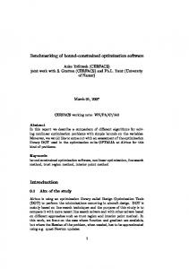
Matchpoint Planet Segment midpoint Impulsive V Segment boundary ΔVN

Smb Smf ΔV3 ΔV2 ΔV1

Fig. 1. Impulsive ∆V transcription of a low-thrust trajectory, after Sims and Flanagan [15]

II. T RAJECTORY M ODEL The trajectory model that is to be used to transcribe an LTMGA trajectory optimization into a nonlinear programming problem (to be solved by global optimization methods) is crucial to the success of the overall algorithm one wants to produce. Criteria to be accounted for include accuracy in the description of the spacecraft dynamics, computational efficiency in the objective function and constraints evaluation, problem dimension and number of nonlinear constraints produced. Bearing these issues in mind, in this paper we propose to use a version of the trajectory model proposed by Sims and Flanagan [15]. Figure 1 briefly illustrates such a trajectory model. Trajectory is divided into legs which begin and end with a planet. Low-thrust arcs on each leg are modeled as sequences of impulsive maneuvers ∆V, connected by conic arcs. We denote the number of impulses (which is the same as the number of segments) with N . The ∆V at each segment should not exceed a maximum magnitude, ∆Vmax , where ∆Vmax is the velocity change accumulated by the spacecraft when it is operated at full thrust during that segment: ∆Vmax = (Tmax /m)(tf − t0 )/N

(1)

where Tmax is the maximum thrust of the low-thrust engine, m is the mass of the spacecraft, t0 and tf is the initial and final time of a leg. At each leg, trajectory is propagated (with a two-body model) forward and backward to a matchpoint (usually halfway through a leg), where the spacecraft state vector becomes Smf = {rx , ry , rz , vx , vy , vz }mf (and similarly for Smb ), where r and v are respectively the position and velocity of the spacecraft and the subscripts represents the Cartesian x, y, z components. The forward- and backward-propagated half-legs should meet at the matchpoint, or the mismatch in position and velocity: Smf − Smb = {∆rx , ∆ry , ∆rz , ∆vx , ∆vy , ∆vz }

(2)

should be less than a tolerance in order to have a feasible trajectory. We employ the patched-conic assumption for gravity-assist trajectories, in which the spacecraft velocity is changed instantaneously by the planet’s gravity during a flyby. The angle between the incoming and outgoing V∞ , or the flyby turn angle δ, is given by: 2 sin(δ/2) = 1/(1 + rp V∞ /µ)

(3)

where rp is the flyby periapsis radius and µ is the gravitational parameter of the gravity-assist body. Note that the constraints on the ∆V magnitude can be considered linear constraints, nonlinear constraints or simply bounds on the decision vector variables according to the exact choice of the decision vector encoding. The resulting NLP will have a dimension equal (or smaller depending on the mission type) to (8 + 3N )M , where M is the number of legs considered, and a number of nonlinear constraints equal

(or greater according to the decision vector encoding chosen and to other mission details) to neq M , where neq is the number of equation considered on the dynamics (e.g. neq = 7 if a three dimensional problem with mass is considered). III. O PTIMIZATION P ROBLEM A. The Objective and Constraints The optimization problem is divided into two phases. In the first phase, we employ global optimization algorithms (which will be discussed in Section IV) to solve the problem in its simpler form, where mass is assumed to be constant throughout the trajectory. The objective is to minimize the total ∆V, or mathematically it can be stated as follow: First Phase with constant mass M in.

J1 =

M X N X j

∆Vi

(4)

i

subject to 1) the equality constraints on the state mismatch in Eq. (2), 2) the inequality constraints that ∆V ≤ ∆Vmax (Eq. (1)), 3) and the inequality constraints that the angle between the incoming and outgoing V∞ vectors is less than the maximum turn angle given by Eq. (3). In the second phase the spacecraft mass is propagated using the rocket equation [16]: mi+1 = mi exp(−∆Vi /g0 Isp )

(5)

where the subscript i denotes the mass and ∆V on the i-th segment, g0 is the standard gravity (9.80665 m/s2 ), and Isp is the specific impulse of the low-thrust engine. In the second phase, the objective is changed from minimizing total ∆V to maximizing the final spacecraft mass: Second Phase with variable mass M ax.

J2 = mf

(6)

where mf is the final spacecraft mass. The constraints here are the same as those in the first phase, except that there is one extra component with the mass (∆m) on the state mismatch vector. Solutions found in the first phase are optimized locally in the second phase using a software package called SNOPT [17] [18], which implements sequential quadratic programming (SQP). B. The Decision Vector The decision vector we used contains the following variables • the departure epoch t0 • the departure velocity relative to the earth V∞ • for each leg j and each segment i, the impulse intensity and direction ∆Vij • for each swingby, the incoming and outgoing velocities relative to the planet • for each swingby j, the swingby epoch tj

the arrival epoch tf All the velocities and impulses are expressed with three Cartesian coordinates. Since we are considering a rendezvous problem, the arrival velocity to the destination is not included in the set of variables, as it is constrained to be zero relative to the planet. During the second phase, additional variables are added to the problem, representing the spacecraft mass at departure and arrival m0 and mf , as well as the spacecraft mass at the swingby times. •

IV. G LOBAL OPTIMIZATION ALGORITHMS The proposed transcription of the LT-MGA problem is a continuous, constrained, nonlinear optimization problem. Since such class of problems usually present local minimizers that are not global, they are often unsolvable using only local optimization algorithms. Practical experience shows that this is usually the case with trajectory optimization problems, regardless of the propulsion type. Thus, local solvers must be used inside a global optimization strategy in order to achieve solutions which are as close as possible to the optimal ones. Here we describe three different approaches that have been tried on such problem. Let us first define some procedures that the algorithms will use. • G() is a procedure that randomly generates a starting point. Ideally, we would like the point to be uniformly distributed on the feasible region, but since our problem’s feasible set is of a very small dimension, and generating a point inside such region is a hard problem by itself, we used a procedure that uniformly generates points into a reasonable box containing the feasible region. • S(x) is a procedure that, given a point x, computes a local minimizer of the objective function, taking x as an initial guess. We used the SNOPT package for our tests [17] [18]. • Best(x, y) is a procedure that, given two solutions x and y, returns the best one according to a fixed rule. Since we are dealing with a constrained optimization problem, Best(x, y) chooses the point with the lower constraint violation norm value. In case both points are feasible, then the point with the lower objective function value is chosen instead. The first and most simple algorithm is called Multistart (MS), which directly optimizes the points obtained by a generator. Multistart can be described by the following pseudo code 1) let x? := G() 2) for i = 1, . . . , N 3) let x := G() 4) let y ? := S(x) 5) let x? := Best(x? , y ? ) 6) end for Although for N big enough and reasonable choices of G, S and Best, Multistart will eventually converge to the global solution, the extremely slow convergence rate renders this algorithm unfit for the vast majority of global

optimization problems. However, because of its simplicity, this algorithm can be effectively used as a baseline to compare other solvers to. The second algorithm is called Monotonic Basin Hopping (BH), or Iterated Local Search[19]. In addition to the procedures previously used by Multistart, Monotonic Basin Hopping needs a procedure P(x) that, given a point x returns another point randomly generated in an conveniently defined neighborhood of x. Such algorithm can then be described as follows 1) let xbest := G() 2) for i = 1, . . . , N 3) let x := G() 4) let x? := S(x) 5) let k := 0 6) while (k < M N I) do: 7) let y := P(x? ) 8) let y ? := S(y) 9) if Best(y ? , x? ) = y ? then 10) let x? := y ? 11) let k := 0 12) else 13) let k := k + 1 14) end if 15) end while 16) let xbest := Best(xbest , x? ) 17) end for In practice, after a local optimization, instead of generating a new point inside the whole feasible region like is done with Multistart, we restrict the generation inside a small region centered on the current best point. If, as it happens with real life problems, the good solutions are clustered together, there is a good chance that the series of perturbations and reoptimizations will lead to the best solution contained inside the cluster [20] [21] [22] [23]. A new point is then generated from the whole feasible set only when no improvement has been made for a given number of times equal to a fixed parameter called Max No Improve (M N I), which has been set to 500 during our runs. The choice of the perturbation function usually determines the Basin Hopping performance. A typical rule is to choose a new point inside a small box or sphere centered on the current point, but problem knowledge, if available, can be used to better tune the perturbation. As an example, when only two different planets are considered, we can expect that by shifting a solution in time by a period equal to the synodic period of such two planets, solutions that are similar (and maybe better) than the current one could be found. So the perturbation rule we used is composed by the following two steps 1) for each variable xi and its lower and upper bounds li and ui , add to xi a value uniformly chosen in the interval [−r(ui − li ), r(ui − li )] with a small given value of r. 2) with a low probability p, shift the solution in time, either forward or backward with equal probability, by

a time length equal to the synodic period. In our experiments, we used r = 0.05 and p = 0.1. Finally, the Simulated Annealing (SA) with Adaptive Neighborhood has been used. The algorithm structure is similar to Monotonic Basin Hopping, with some important differences in key parts of the algorithm, which are quickly described here. For a more complete description we refer to [24] [25]. First of all, the comparison in line 9 is modified to allow for non monotonicity. The problem is transformed to an unconstrained optimization problem by using a penalty function to account for constraints violations. Then, Best(x, y) returns x with probability 1 if f (x) ≤ f (y), or with probability e(f (y)−f (x))/T if f (x) > f (y). T is the temperature parameter, which is exponentially decreased every fixed number of iterations. Furthermore, the perturbation procedure P is adaptive, meaning that the radius of the perturbation is adjusted at every iteration. Such r value is increased each time the generated point is accepted, and decreased each time the point is refused. Finally, the local optimization S is not executed at each step of the algorithm, but just once at the end, starting from the point returned by the Simulated Annealing with Adaptive Neighborhood.

problem which minimizes the total ∆V (see Eq. (4)) and mass is excluded in the calculations. The dimension of this problem is 75 and there are 35 nonlinear constraints (as we choose cartesian coordinates to encode the ∆V the constraint on their magnitude is quadratic and thus increase the number of nonlinear constraints). We first let the global optimizers run for a fixed time (∼100 mins) on a PC (AMD [email protected] GHz with 3GB of RAM) which produces hundreds of trajectories. To select promising solutions for the second phase of the problem, we only consider solutions that has a norm on the constraint violation vector less than 10−6 , which reduces the number of solutions to less than a hundred. Table II summarizes the characteristics of the selected solutions found in the first phase. TABLE II O PTIMAL T OTAL ∆ V (P HASE 1) FOR THE E-E-J M ISSION ( KM / S )

Algorithm Basin Hopping Simulated Annealing Multi-Start

Best

Worst

Mean

Std

9.558 9.940 9.584

20.933 13.971 20.239

10.954 11.623 12.133

1.861 1.290 2.018

No. of Solutions 44 18 50

TABLE III O PTIMAL F INAL M ASS (P HASE 2) FOR THE E-E-J M ISSION ( KG )

V. N UMERICAL R ESULTS A. Nuclear Electric Propulsion Mission to Jupiter

Algorithm

We demonstrate the application of our global optimization framework to perform preliminary design of trajectories for a mission that employs nuclear electric propulsion (see Table I). The spacecraft is assumed to have a thruster with a constant maximum thrust and a constant specific impulse, with similar hardware parameters to the Jupiter Icy Moons Orbiter [26][27] [28] [29] [30] (a canceled mission originally proposed by NASA in 2003). We consider two planetary encounter sequences in our example scenario: Earth-EarthJupiter and Earth-Earth-Earth-Jupiter (i.e., one or two Earth flybys), in which both cases rendezvous at Jupiter.

Basin Hopping Simulated Annealing Multi-Start

90

Worst

Mean

Std

17, 004 16, 927 16, 995

16, 200 15, 795 14, 385

16, 720 16, 459 16, 338

203 326 517

No. of Solutions 40 18 45

BH SA MS

80

Percentile of Solutions

TABLE I PARAMETERS FOR A N UCLEAR E LECTRIC P ROPULSION M ISSION

100

Best

70 60 50 40 30 20 10

Parameters Initial mass of the spacecraft Maximum thrust Specific impulse Launch date Launch V∞ Maximum time of flight Minimum flyby radius

Values 20, 000 kg 2.26 N 6, 000 s Jan. 1, 2020 – Jan. 1, 2030 ≤ 2.0 km/s 10 years (E-E-J) or 15 years (E-E-E-J) 7, 000 km

B. Earth-Earth-Jupiter Our approach begins with the three global optimizers solving a simplified form of an Earth-Earth-Jupiter rendezvous

0 1.7

Fig. 2.

1.69

1.68

1.67

1.66

1.65

1.64

Final Mass, kg

1.63

1.62

1.61

1.6 4 x 10

Cumulative percentile of optimal solutions for the E-E-J mission

In the second phase, we perform local optimization to maximize the final mass (see Eq. (6)) on the selected solutions found by the three global optimizers and the results are shown in Table III. We notice that some of the solutions in Table II fail to converge in the second phase (and therefore the number of solutions in Table III is less). An unpaired student’s t-test is performed on the results found by the 3

different Earth-Earth resonance transfer orbit. For example, 1:1 resonance with flight time ∼400 days, 2:3 resonance with flight time ∼800 days, and 3:2 resonance with flight time ∼1100 days. Unlike the case in the ballistic transfer, in the low-thrust transfer case, the Earth-Earth flight time does not exactly equal to some integer multiple of Earth’s orbital period and the spacecraft does not encounter the Earth at the same position from launch. However the mechanism in the low-thrust case is similar to the chemical case [31], where the V∞ at the second Earth encounter is increased through some small maneuvers. 4

1.75

x 10

1.7 1.65

Final Mass, kg

algorithms to test for statistical significance. We found that the results found by Basin Hopping are statistically different from those returned by the other two algorithms, while results found by Simulated Annealing and Multi-Start are not. The conclusion from the unpaired student’s t-test is consistent with the cumulative percentile curve shown in Fig. 2, in which results found by Basin Hopping always have higher final mass than the other two methods, while Simulated Annealing and Multi-Start have similar performance. Figure 3 plots the x-y projection of a trajectory found by Basin Hopping with the highest final mass. On the plot, the solid and dash curves represent thrusting and coasting segments, respectively; while a ∆V is shown as an arrow in the midpoint of a segment. In this example, the spacecraft leaves the Earth on October 15, 2022 with a V∞ of 2 km/s. It enters an 3:2 resonance orbit with a period of ∼ 1.5 years and goes around the Sun for 2 revs, before it flybys the Earth after 2.9 years with an increased V∞ of 9.0 km/s. After the gravity assist at the Earth, its aphelion increases for the transfer to Jupiter. According to the numerical results, the spacecraft rendezvous at Jupiter on October 2030. However, we notice that the ∆V on the last two segments are zero (i.e., coasting segments), which means the spacecraft has actually arrived at Jupiter on September 2029, about one year earlier than the numerical results. This is merely a minor numerical issue which does not affect the validity of the solution.

1.6 1.55 1.5 BH SA MS

1.45 1.4 0

5

500

1000

1500

2000

2500

3000

3500

4000

Launch Date, days since Jan. 1, 2020

4

Fig. 4.

3

Optimal E-E-J solutions with various launch dates

2 4

y, AU

1

1.75

x 10

Earth launch

0

Earth flyby

-1

1.7

-2

-4 Jupiter rendezvous (numerical)

-5 -6

-4

-2

0

x, AU

2

4

6

Final Mass, kg

1.65 Jupiter rendezvous (actual)

-3

1.6 1.55 1.5

Fig. 3.

Trajectory plot of an Earth-Earth-Jupiter rendezvous mission BH SA MS

1.45

Besides the value of the objective function, it is also interesting from a mission design point-of-view that the optimization process is able to find trajectories that launches on different dates. In our example in Fig. 4, the difference in the final mass is less than 200 kg (or 1% of the initial mass) for most launch periods. The 1% penalty of the final mass gives flexibility to the mission designer to choose a different date in case there is a change in the mission. The process is also able to locate various locally optimal trajectory families, which is interesting from an astrodynamics point-of-view. From Fig. 5, we note that the ‘clusters’ of solutions belongs to

1.4 200

Fig. 5.

400

600

800

1000

1200

Time of Flight of the First Leg, days

1400

Optimal E-E-J solutions with various Earth-Earth transfer times

C. Earth-Earth-Earth-Jupiter In the second example, we examine trajectories with two Earth swingbys. In comparison with the first case, the dimension of the problem increases to 112 with 56 nonlinear

constraints. We let the global optimizers run for 1,000 mins and found a few thousands trajectories, in which only a few hundreds of solutions that has a norm on the constraint violation vector less than 10−6 are further optimized for the final mass. Results from the first and second phases are summarized in Fig. 6 and Tables IV and V.

increased to 9.0 km/s. For the arrival at Jupiter, since the ∆V on the last 5 segments are zero, the spacecraft actually rendezvous at Jupiter 4.5 years early than stated numerically, which means the toal flight time of the trajectory is 8.0 years. Comparing with the E-E-J trajectory in Fig. 3, the addition of one Earth flyby increases the time of flight for one year, while having the benefit of a higher final mass of ∼600 kg.

TABLE IV O PTIMAL T OTAL ∆ V (P HASE 1) FOR THE E-E-E-J M ISSION ( KM / S )

5

Rendezvous (numerical)

4

Algorithm

Worst

Mean

Std

7.524 8.618 7.869

38.280 30.594 31.438

11.242 14.120 12.837

3.639 4.726 3.516

No. of Solutions 488 66 204

3 2 1

y, AU

Basin Hopping Simulated Annealing Multi-Start

Best

TABLE V O PTIMAL F INAL M ASS (P HASE 2) FOR THE E-E-E-J M ISSION ( KG )

Flyby2

0 -1

Flyby1

Launch

-2 -3

Algorithm

Best

Basin Hopping Simulated Annealing Multi-start

Worst

17, 601 17, 282 17, 307

11, 681 15, 144 12, 602

Mean

Std

16, 609 16, 249 16, 214

932 606 637

No. of Solutions 239 29 129

-4

Rendezvous (actual)

-5 -6

-4

-2

0

x, AU

2

4

6

Fig. 7. Trajectory plot of an Earth-Earth-Earth-Jupiter rendezvous mission 100 90

BH SA MS

Percentile of Solutions

80 70 60 50 40 30 20 10 0 1.76

1.74

1.72

1.7

1.68

1.66

1.64

Final Mass, kg

1.62

1.6

1.58

1.56 4 x 10

VI. C ONCLUSIONS We successfully apply global optimization techniques to achieve the automated design of two instances of multiple gravity assist low-thrust interplanetary trajectories within a ten year wide launch window. The use of our technique is not limited to the two particular problems here studied as it rests upon a general interface between the Sims-Flanagan trajectory model and a global optimization layer hybridized with a local search as to deal efficiently with the nonlinear constraints. The resulting method makes no use of expert knowledge and starts from randomly generated trajectories, thus achieving a completely automated design process.

Fig. 6. Cumulative percentile of optimal solutions for the E-E-E-J mission

R EFERENCES

As in the case of the E-E-J example, the Basin Hopping algorithm surpasses the other two in terms of the quality (objective) and quantity (number of solutions) of its solutions. However we note that in this example, only ∼40-60% of solutions found in the first phase are able to converge in the second phase. The reason for the decrease in the convergence rate is most likely due to the increase in the complexity of the problem (an extra flyby is added) that makes accounting for the mass important already in the first optimization loop. The trajectory of the ‘best’ solution (with the highest final mass) found by Basin Hoppoing is plotted in Fig. 7. Here the spacecraft first performs a 1:1 resonance transfer for 495 days on the first leg, where the V∞ is boosted from 2.0 to 5.3 km/s. After the first flyby, it enters a 2:1 resonance orbit where it reencounters the Earth after 772 days and the V∞ is further

[1] P. Di Lizia and G. Radice, “Advanced Global Optimisation Tools for Mission Analysis and Design,” European Space Agency, the Advanced Concepts Team, Tech. Rep. 03-4101b, 2004. [2] D. Myatt, V. Becerra, S. Nasuto, and J. Bishop, “Advanced Global Optimisation Tools for Mission Analysis and Design,” European Space Agency, the Advanced Concepts Team, Tech. Rep. 03-4101a, 2004. [3] D. Izzo, V. Becerra, D. Myatt, S. Nasuto, and J. Bishop, “Search Space Pruning and Global Optimisation of Multiple Gravity Assist Spacecraft Trajectories,” Journal of Global Optimization, vol. 38, no. 2, pp. 283– 296, 2007. [4] T. Vinko and D. Izzo, “Global Optimisation Heuristics and Test Problems for Preliminary Spacecraft Trajectory Design,” European Space Agency, the Advanced Concepts Team, Tech. Rep. GOHTPPSTD, 2008. [5] M. Vasile and P. De Pascale, “Preliminary Design of Multiple GravityAssist Trajectories,” Journal of Spacecraft and Rockets, vol. 43, no. 4, pp. 794–805, 2006. [6] R. Armellin, P. Di Lizia, F. Topputo, M. Lavagna, F. Bernelli-Zazzera, and M. Berz, “Gravity Assist Space Pruning Based on Differential Algebra,” Celestial Mechanics and Dynamical Astronomy, vol. 106, no. 1, pp. 1–24, 2010.

[7] D. Izzo. (2009, Jun.) Global Trajectory Optimization Competition portal. [Online]. Available: http://www.esa.int/gsp/ACT/mad/op/GTOC/index.htm [8] D. Izzo, T. Vinko, and M. Zapatero. (2009, Jun.) Global Trajectory Optimization Competition Database. [Online]. Available: http://www.esa.int/gsp/ACT/inf/op/globopt.htm [9] B. Addis, A. Cassioli, M. Locatelli, and F. Schoen, “Global Optimization for the Design of Space Trajectories,” Computational Optimization and Applications, 2008. [10] A. Cassioli, D. Di Lorenzo, M. Locatelli, F. Schoen, and M. Sciandrone, “Machine Learning for Global Optimization,” Technical Report 2360, Optimization Online, 2009, Tech. Rep., 2009. [11] O. Sch¨utze, M. Vasile, O. Junge, M. Dellnitz, and D. Izzo, “Designing Optimal Low-Thrust Gravity-Assist Trajectories Using Space Pruning and a Multi-Objective Approach,” Engineering Optimization, vol. 41, no. 2, pp. 155–181, 2009. [12] K. Alemany and R. Braun, “Survey of Global Optimization Methods for Low-thrust, Multiple Asteroid Tour Missions,” presented at the AAS/AIAA Space Flight Mechanics Meeting, Jan. 2007, paper AAS 07-211. [13] C. H. Yam, F. Biscani, and D. Izzo, “Global Optimization of LowThrust Trajectories via Impulsive Delta-V Transcription,” presented at the 27th International Symposium on Space Technology and Science, July 2009, paper ISTS 2009-d-03. [14] M. A. Vavrina and K. C. Howell, “Global Low-Thrust Trajectory Optimization through Hybridization of a Genetic Algorithm and a Direct Method,” presented at the AIAA/AAS Astrodynamics Specialist Conference, Aug. 2008, paper AIAA 2008-6614. [15] J. A. Sims and S. N. Flanagan, “Preliminary Design of Low-Thrust Interplanetary Missions,” presented at the AAS/AIAA Astrodynamics Specialist Conference, Aug. 1999, paper AAS 99-338. [16] K. E. Tsiolkovsky, “Exploration of the Universe with Reaction Machines (in Russian),” The Science Review, vol. 5, 1903. [17] W. Gill, P. E.and Murray and M. A. Saunders, “SNOPT: An SQP Algorithm for Large-Scale Constrained Optimization,” SIAM Journal on Optimization, vol. 12, no. 4, pp. 979–1006, 2002. [18] P. E. Gill, W. Murray, and M. A. Saunders, User’s Guide for SNOPT Version 7, Software for Large-Scale Nonlinear Programming, Stanford Business Software Inc., Feb 2006. [Online]. Available: www.sbsi-sol-optimize.com [19] H. R. Lourenc¸o, O. C. Martin, and T. St¨ulze, “Iterated Local Search,” in Handbook of Metaheuristics, F. W. Glover and G. A. Kochenberger, Eds. Boston, Dordrecht, London: Kluwer Academic Publishers, 2003, pp. 321–353. [20] D. J. Wales and J. P. K. Doye, “Global Optimization by BasinHopping and the Lowest Energy Structures of Lennard–Jones Clusters Containing up to 110 Atoms,” Journal of Physical Chemistry A, vol. 101, no. 28, pp. 5111–5116, 1997. [21] D. J. Wales and H. A. Scheraga, “Global Optimization of Clusters, Crystals, and Biomolecules,” Science, vol. 285, pp. 1368–1372, 1999. [22] R. H. Leary, “Global Optimization on Funneling Landscapes,” Journal of Global Optimization, vol. 18, pp. 367–383, 2000. [23] A. Grosso, A. Jamali, M. Locatelli, and F. Schoen, “Solving the Problem of Packing Equal and Unequal Circles in a Circular Container,” Journal of Global Optimization, July 2009. [Online]. Available: http://www.springerlink.com/content/r71v580u762633u2/ [24] S. Kirkpatrick, C. D. Gelatt, Jr., and M. P. Vecchi, “Optimization by Simulated Annealing,” Science, vol. 220, pp. 671–680, 1983. [25] A. Corana, M. Marchesi, C. Martini, and S. Ridella, “Minimizing Multimodal Functions of Continuous Variables with the ‘Simulated Annealing’ Algorithm,” ACM Transactions on Mathematical Software (TOMS), vol. 13, no. 3, p. 280, 1987. [26] R. Greeley and E. Johnson, T., “Report of the NASA Science Definition Team for the Jupiter Icy Moons Orbiter,” NASA Science Definition Team, Tech. Rep., Feb. 2004. [27] G. J. Whiffen, “An Investigation of a Jupiter Galilean Moon Orbiter Trajectory,” presented at the AAS/AIAA Astrodynamics Specialist Conference, Aug. 2003, paper AAS 03-554. [28] C. H. Yam, T. T. McConaghy, K. J. Chen, and J. M. Longuski, “Preliminary Design of Nuclear Electric Propulsion Missions to the Outer Planets,” presented at the AIAA/AAS Astrodynamics Specialist Conference, Aug. 2004, paper AIAA 2004-5393. [29] C. H. Yam, T. T. McConaghy, K. J. Chen, and M. Longuski, J., “Design of Low-Thrust Gravity-Assist Trajectories to the Outer Planets,”

presented at the 55th International Astronautical Congress, Oct. 2004, paper IAC-04-A.6.02. [30] D. W. Parcher and J. A. Sims, “Gravity-Assist Trajectories to Jupiter Using Nuclear Electric Propulsion,” presented at the AAS/AIAA Astrodynamics Specialist Conference, Aug. 2005, paper AAS 05-398. [31] N. J. Strange and J. A. Sims, “Methods for the Design of V-Infinity Leveraging Maneuvers,” presented at the AAS/AIAA Astrodynamics Specialist Conference, July/Aug. 2001, paper AAS 01-437.