IEEE TRANSACTIONS ON IMAGE PROCESSING
1
Constrained Multi-view Video Face Clustering Xiaochun Cao, Changqing Zhang , Chengju Zhou, Huazhu Fu, Hassan Foroosh
Abstract—In this paper, we focus on face clustering in videos. To promote the performance of video clustering by multiple intrinsic cues, i.e., pairwise constraints and multiple views, we propose a Constrained Multi-view Video Face Clustering (CMVFC) method under a unified graph-based model. First, unlike most existing video face clustering methods which only employ these constraints in the clustering step, we strengthen the pairwise constraints through the whole video face clustering framework, both in sparse subspace representation and spectral clustering. In the constrained sparse subspace representation, the sparse representation is forced to explore unknown relationships. In the constrained spectral clustering, the constraints are used to guide for learning more reasonable new representations. Second, our method takes into account both the video face pairwise constraints as well as the multi-view consistence simultaneously. Specifically, the graph regularization enforces the pairwise constraints to be respected and the co-regularization penalizes the disagreement among different graphs of multiple views. Experiments on three real-world video benchmark datasets demonstrate the significant improvements of our method over the state-of-the-art methods. Index Terms—Video face clustering, pairwise constraints, sparse subspace representation, multi-view clustering
I. I NTRODUCTION Video face clustering aims to divide the facial images into different subsets according to different persons. This technique can be used in many applications, such as video summarization [1], [2], automatic cast listing in feature-length films [3], [4], and automatic collection of large-scale face datasets [5], [6]. However, the task of video face clustering is still very challenging for the following reasons. First, in realworld videos, the appearances of faces often vary significantly due to the lighting conditions, especially light angles which often change drastically. Second, one person might have very different facial expressions and head poses, which change the appearances of faces. Moreover, partial occlusions and hair This work was supported by National Natural Science Foundation of China (No. 61332012 and No. 61100121), National Basic Research Program of China (2013CB329305), National High-tech R&D Program of China (2014BAK11B03), and 100 Talents Programme of The Chinese Academy of Sciences. Hassan Foroosh was supported in part by the National Science Foundation under grant IIS-1212948. (Corresponding author: Changqing Zhang). X. Cao is with School of Computer Science and Technology, Tianjin University, Tianjin 300072, and State Key Laboratory of Information Security, Institute of Information Engineering, Chinese Academy of Sciences, Beijing 100093, China (E-mail:
[email protected]). C. Zhang and C. Zhou are with School of Computer Science and Technology, Tianjin University, Tianjin 300072, China (E-mail:
[email protected],
[email protected]). H. Fu is with School of Computer Engineering, Nanyang Technological University, Nanyang Avenue 639798, Singapore (E-mail:
[email protected]). H. Foroosh is with Computational Imaging Laboratory (CIL) of the School of EECS at the University of Central Florida (UCF), Orlando, Florida. (Email:
[email protected])
.
style changes in the video also increase the difficulties for video face clustering. Traditional image-based face clustering methods often distinguish different individuals only based on the facial similarities. In video face clustering, there is some prior knowledge which can be used to improve the performance. Cour et al. [7] use scripts and subtitles to obtain the cues as to which characters are present. These cues for character presence are then combined with facial similarities to help face clustering. However, this text-based information is not always available. In contrast, there are two pairwise constraints inherent in videos, i.e., faces from the same face track are likely to be from the same person, while faces can not be from the same person if they appear together in the same video frame. These two constraints are named as MUST-LINK and CANNOT-LINK constraints, respectively. Some existing methods [3], [5], [6] use these constraints in video face clustering, and demonstrate their values. However, these methods only consider these constraints in clustering, and ignore the constraints in representation. In our work, we take advantage of them in the sparse subspace representation to better explore unknown face relationships. Afterwards, the constraints are reused in the spectral clustering step to ensure more accurate clustering result. On the other hand, traditional face clustering/recognition methods mainly focus on obtaining a good distance metric for representing the structure of inter-personal dissimilarities and intra-personal similarities [3], [5], [8], [9], [10]. However, the metric-based clustering methods are sensitive to the quality of videos since they always have a huge uncertainty in realworld cases. To relieve this limitation, we make use of multiple features simultaneously. These features often describe facial images from different views. Although individual views might not be sufficient on their own to give a good enough clustering result, they often provide complementary information to each other which can lead to improved performance on the clustering task. Recently, the efficiency of the multi-view methods has been demonstrated [11], [12], [13]. However, most multi-view methods do not consider the prior constraints in clustering, which are usually critical in many applications. In this paper, we introduce pairwise constraints into the multi-view clustering to effectively exploit the complementary information in different views. In this paper, we provide a Constrained Multi-view Video Face Clustering (CMVFC) method, which combines the pairwise constraints in both sparse subspace representation and spectral clustering procedures. Moreover, we also introduce the multi-view clustering fashion to exploit multiple features. We effectively exploit the pairwise constraints and the multi-view consistence as regularization simultaneously. The experiments show that the proposed method outperforms the state-of-the-
2
IEEE TRANSACTIONS ON IMAGE PROCESSING
(e) Clustering restult
(a) Input Video
Histogram Intersection Cannot-link
Frame Overlap
CL Matrix
Face Track
ML Matrix
Must-link
Frames
Constrained Multi-view Video Clustering
Pairwise Constraints LBP
GABOR
UJACI
LBP 1 1 0 0 0
0 0
1 1 0 0 0
0 0
0 0 1 1 1
0 0
0 0 1 1 1
0 0
0 0 1 1 1
0 0
Faces
Face Alignment
(b) Face detection
0 0 0 0 0
1 1
0 0 0 0 0
1 1
+
0 0 ‐1 ‐1 ‐1 0 0 ‐1 ‐1 ‐1 ‐1 ‐1 0 0 0
0 0 0 0 0 0
‐1 ‐1 0 0 0 ‐1 ‐1 0 0 0
0 0 0 0
0 0 0 0 0 0 0 0 0 0
0 0 0 0
=
X
X GABOR = Constrained Sparse Representation
Multiple Features (c) Feature & Constraint extraction
(d) Representation & Clustering
Fig. 1. The framework of our method. From the input video (a), we extract the frames and detect the facial images (b). Then, we build up the must-link matrix based on the face tracks and cannot-link matrix based on the frames. Meanwhile, we extract the multiple features for the detected facial images (c). Based on these constraints and features, we perform our CMVFC algorithm in two steps, constrained sparse representation and constrained spectral clustering (d) to get the clustering result (e).
art methods on three real-world benchmark datasets. II. R ELATED W ORK We give a brief introduction about some face clustering techniques and some general clustering methods based on sparse subspace representation or multiple views, which are highly related to our work. Video face clustering: Most existing video face clustering methods focus on obtaining a good representation for the structure of inter-personal dissimilarities. For example, Fitzgibbon et al. [3], [5] proposed an affine invariant distance metric which is robust to a desired group of transformations for video face clustering. Huang et al. [14] proposed to cluster faces with multi-views in a video sequence. They clustered video faces based on pose grouping results. The multi-view in their work is a concept in geometry rather than descriptor. The work [15] measures the face similarity by mutual information and its extension [16] incorporates pairwise constraints directly, replacing the elements of similarity matrix with 1 for mustlink and 0 for cannot-link pairs. A more recent work on video face clustering with pairwise constraints is presented in [6], which incorporates pairwise constraints within a Hidden Markov Random Fields. However, this work only utilizes the pairwise constraints in clustering procedure with single feature. In contrast, we use pairwise constraints in both sparse subspace representation and spectral clustering to fully explore the constraints. Moreover, we cluster the facial images under a multi-view framework to exploit the complementary information. Constrained clustering: Clustering with pairwise constraints has been attracting more and more attentions in the machine learning and data mining communities. Generally, there are two categories of methods using pairwise constraints in clustering. The first category introduces the metric learning fashion which aims to learn a Mahalanobis distance that
minimizes the distance between must-link samples and maximizes the distance between cannot-link samples. However, the metric learning step and clustering step are often isolated in these methods, and thus the performance cannot be guaranteed [6]. The second category adopts the traditional centroid-based clustering methods, such as K-means [17], [18] or Gaussian mixtures [19] to meet the pairwise constraints. There exist few works to blend the pairwise constraints in a natural way. The work in [20] simply uses the Gaussian kernel as the affinity but replaces entries for must-link pairs with 1 and cannot-link pairs with 0. The work in [21] combines must-link and cannotlink affinity by propagating the pairwise constraints over the original affinity matrix. Instead of directly modifying the affinity matrix [20], [21], we utilize the pairwise constraints as regularization into spectral clustering which directly aims to obtain a more reasonable representation. Multi-view clustering: Multi-view clustering is of great importance since an abundance of complementary perspectives and multi-view representations of data are often available. The method in [12] develops multi-view spectral clustering via generalizing the normalized cut from a single view to multiple views. The authors gave a random walk based formulation for the problem. The clustering algorithm in [22] creates a bipartite graph and is based on the minimizing-disagreement. However, it concentrates on the data with only two views. The method in [11] uses Linked Matrix Factorization to fuse the information from multiple graph sources. The authors in [13] proposed a spectral clustering framework which co-regularizes the clustering hypotheses, and propose the co-regularization scheme to penalize the disagreement across different views. The method in [23] employs Hilbert Schmidt Independence Criterion (HSIC) to enhance the complementarity across different views. Our method introduces the pairwise constraints into multi-view spectral clustering in an elegant manner, which effectively exploits the pairwise constraints and the multi-view
CAO et al.: REGULAR PAPER
consistence simultaneously. Sparse subspace representation: There has been a great interest in sparse representation during the last decade. Wright et al. [24] use `1 -norm minimization to deal with missing or corrupted data in face recognition. Most of the sparse representation literature assumes that the data lie in a single linear subspace. Furthermore, [25], [26] propose to use the sparse representation of vectors lying on a union of subspaces to cluster the data into separated subspaces. However, these methods do not consider prior constraints in representation. In this paper, we introduce pairwise constraints into sparse subspace representation, aiming to better explore the face relationships for clustering. Image set based face recognition: There are some face recognition methods focusing on learning over facial image sets [27], [28], [29], [30], [31], [32], [33], [34], [35], in which each test and training example is a set of images of an individual’s face. These methods usually try to design or learn different similarity metrics for matching image sets (e.g., canonical angles between two subspaces [29]). A video face track can be regarded as a facial image set. Therefore, the set models (e.g., modeling each image set as a manifold [30]) in these methods can be employed to represent face tracks. Consequently, the corresponding similarity metrics for image set can be utilized to cluster these face tracks. III. F RAMEWORK OF O UR A PPROACH Fig. 1 shows the framework of our method. Given the input video, we extract the faces for each frame, as shown in Fig. 1 (b). In our work, we employ face detector to get an initial face set. The face tracking technique is employed to link the detected face. After detecting the faces, we align them and extract the features of each facial image. The constrained matrix as shown in Fig. 1(c) is built up based on the must-link and cannot-link constraints. Next, the sparse representation with these constraints is provided to obtain the sparse coefficient matrix corresponding to each feature as shown in Fig. 1(d). Finally, based on these constrained sparse representations, we apply multi-view spectral clustering with pairwise constraints on the similarity matrix to get the final clustering result. A. Preprocessing For face detection, one of the most important method is proposed by Viola and Jones [36], which builds a successful face detector running in real time. Any or more advanced similar works can be easily integrated into our approach. We employ the face tracking method in [37], which consists of two metrics: histogram intersection and frame overlap. For face alignment, the work in [38] which jointly aligns complex images in a unsupervised manner is employed in our framework. It has shown high quality results on the faces in the Wild dataset [39], which is also under large variation of head poses, lighting conditions, backgrounds as in the realworld videos. To concentrate on face clustering approach, in our work, we assume that a set of face windows are well extracted. The preprocessing is similar to other video face
3
clustering methods [6], [40]. First, most false positives of face detections can be easily eliminated by selecting the tracks with a sufficiently large number of faces. Second, we manually select the tracks corresponding to main characters to eliminate the wrong detections. B. Pairwise constraints Given a set of facial images F = {f1 , f2 , ..., fn }, where n is the number of the total faces, we extract a d-dimensional feature vector xi ∈ Rd for each image fi , forming the corresponding feature matrix X = [x1 , x2 , ..., xn ]. Two matrices are built up to describe the pairwise constraints of the faces, i.e., the must-link matrix M ∈ Rn×n and the cannot-link matrix C ∈ Rn×n . The matrix M represents the must-link constraints, where the elements corresponding to the face pairs in the same track are set to 1 while others are set to 0. The matrix C represents the cannot-link constraints, the elements of which corresponding to the face pairs belonging to the overlapped tracks are set to -1 while others are set to 0. For convenience, we also define M = {(xi , xj ) ∈ M|mij = 1} and C = {(xi , xj ) ∈ C|cij = −1} as the sets of the must-link and cannot-link constraints, respectively. C. Constrained sparse subspace representation Ideally, the face xi can be sparsely represented by a small subset of facial images from the same person in the dataset [24], [25]. The relationship can be written as xi = Xai s. t. aii = 0,
(1)
where ai = [a1i , a2i , ..., ani ]T , and the constraint aii = 0 eliminates the trivial solution of representing a facial image with itself. The coefficient vector ai should have nonzero entries for a few facial images from the same person and zeros from the rest. In other words, the matrix X is a self-expressive dictionary in which each facial image can be represented by a linear combination of the others. Some relationships among faces have been known from the must-link and the cannot-link constraints. Therefore, we pay attention to exploring the unknown relationships by utilizing the prior constraints xi = Xai s. t. aji = 0, ∀(xj , xi ) ∈ M ∪ C.
(2)
The reason to eliminate the aji for (xj , xi ) ∈ M is to avoid the representation using faces in the same track. Consequently, the sparse representation is forced to relate the faces with unknown relationships. The reason to eliminate the aji for (xj , xi ) ∈ C is to avoid the representation between faces in the same video frame. On the other hand, the known must-link and cannot-link constraints are later re-exploited in spectral clustering (Eq. (13)). One limitation of Eq. (2) is that the representation of xi in the dictionary X is not unique in general. Since we are interested in efficiently finding a nontrivial sparse representation of xi in the data set X, we use the tightest convex relaxation of the `0 -norm, i.e.,
min ai 1 (3) s. t. xi = Xai and aji = 0, ∀(xj , xi ) ∈ M ∪ C.
4
IEEE TRANSACTIONS ON IMAGE PROCESSING
Moreover, considering clustering of data points that are contaminated with sparse outlying entries and noise [25], the constrained sparse representation is obtained by the following equation
min ai + λe ||ei ||1 + λz ||zi ||2
For the k-way spectral clustering with a single view, we aim to obtain a new embedding representation U of the original data X by optimizing the following objective function [44] argmax T r(UT LU) U∈Rn×k T
1
s. t. xi = Xai + ei + zi and aji = 0, ∀(xj , xi ) ∈ M ∪ C, (4) where ei ∈ Rd and zi ∈ Rd are the error and noise, respectively. The two parameters λe and λz balance the three terms in Eq. (4). Without loss of generality, we can rewrite the sparse optimization problem (4) for all faces in the following matrix form
min A + λe ||E||1 + λz ||Z||2F 1
s. t. X = XA + E + Z and aji = 0, ∀(xj , xi ) ∈ M ∪ C, (5) where A = [a1 , a2 , ..., an ] ∈ Rn×n is the coefficient matrix, the ith column of which corresponds to the sparse representation of xi . More specifically, each column of A corresponds to a new representation of a facial image, whose nonzero elements ideally correspond to faces from the same person. Since the optimization problem in Eq. (5) is convex with respect to the variables A, E and Z, it can be solved efficiently using convex programming tools [41], [42].
D. Constrained spectral clustering Before introducing the multi-view clustering, we first depict our face clustering method using the single feature in this subsection. With Eq. (5), we obtain a sparse coefficient matrix A for the whole facial image set. Afterwards, we build a weighted graph G = (V, E, W), where V denotes the set of n nodes in graph G corresponding to the set of n faces, and E denotes the edges between nodes. W ∈ Rn×n is a symmetric nonnegative similarity matrix representing the weights of the edges. Typically, an ideal similarity graph G should have connections corresponding to the same person and have no connections corresponding to different persons. In the sparse representation solution A from subsection III-C, nonzero elements can be regarded as a measurement of the relationships between faces. This provides a choice of constructing the similarity matrix [25], W = |A| + |A|T .
(6)
We normalize A as ai ← ai /kai k∞ to make sure the weights in similarity graph are of the same scale. A straightforward combination way [43] is incorporating the must-link and cannot-link constraints into the similarity matrix directly. It can be written as Wpc = W + ζM + ηC,
(7)
where the trade-off factors ζ and η encode the belief degrees for the must-link and cannot-link constraints, respectively. However, instead of directly combining the two pairwise constraint matrices into the similarity matrix, we regularize the pairwise constraints in spectral clustering which directly aims to obtain a more reasonable embedding representation.
(8)
s. t. U U = I, where L = D−1/2 WD−1/2 is the normalized graph Laplacian matrix, and D is a diagonal matrix with element dii = Pn j=1 wij . For convenience, we denote di = dii . W is the similarity matrix, which is often constructed by the original feature X. T r(·) denotes the trace of a matrix. Note that, different from the work in [13], we use the constrained sparse subspace representation in Eq. (6) to construct the similarity matrix W instead of the original feature based on Euclidean distance or kernels. Therefore, the pairwise constraints are incorporated into the similarity matrices to boost the clustering performance. With each row of U = [u1 , u2 , ..., un ]T acting as a new representation of an original data point, we cluster them into k clusters with K-means algorithm. Considering the pairwise constraints, a regularized term is designed to ensure that the representation of must-link pairs are close and the representation of cannot-link pairs are far away from each other. We denote the distance of two points ui and uj according to the two constraint matrices, M and C, as follow uj ui −q ||2 , (9) dml (ui , uj ) = || p ml di dml j and
ui uj dcl (ui , uj ) = || q − q ||2 , cl d¯cl d¯i j
(10)
ml ¯cl where the distance is normalized by dml (d¯cl (dj ) i i ) and dj in order to reduce the impact of popularity of nodes as in traditional graph-based learning [45], [46], and the effectiveness of the normalized technique is well proved. Accordingly, the pairwise constraints as regularization is defined as:
R(U; M, C) =
+
n 1 X ui uj || p ||2 mij −q ml 2 i,j=1 di dml j n uj 1 X ui || q − q ||2 cij 2 i,j=1 d¯cl d¯cl j i
¯ cl )U), = T r(UT (I − Lml )U) + T r(UT (I − L (11) where Lml is the normalized graph Laplacian matrix corresponding to the must-link constraint matrix M. Note that ¯ cl = D¯cl −1/2 CD¯cl −1/2 as the new graph we denote L Laplacian corresponding to the cannot-link matrix C with Pn ¯ cl cl ¯ di = dii = j=1 |cij |. The absolute operator is to handle a graph with negatively weighted edges, which is proved by [47]. By ignoring the constant additive term, Eq. (11) can be rewritten as: ¯ cl U). R(U; M, C) = −T r(UT Lml U) − T r(UT L
(12)
Intuitively, minimizing the term in Eq. (12) will enforce
CAO et al.: REGULAR PAPER
the new representation U to simultaneously meets the graphs corresponding to the must-link matrix M and the cannot-link matrix C. For our constrained clustering method, we combine the pairwise constraint regularization in Eq. (12) into Eq. (8) as a new objective function
5 T
we have WU(v) = U(v) U(v) and ||WU(v) ||2F = k, where k is the number of clusters. The Eq. (15) can be rewritten as follow by ignoring the constant additive and scaling terms T
T
D(U(v) , U(w) ) = −T r(U(v) U(v) U(w) U(w) ).
(16)
The term should be minimized to ensure the clustering consis¯ cl U) tence across all the different views. For our constrained multiargmax T r(UT LU) + λml T r(UT Lml U) + λcl T r(UT L U∈Rn×k view spectral clustering method, we combine the disagreement penalty term D(·) in Eq. (16) and the constraint regularization s. t. UT U = I, (13) term R(·) in Eq. (12) into Eq. (8), then the new objective where λml and λcl encode the different belief degrees for function, i.e., constrained multi-view spectral clustering is the must-link and cannot-link constraints, respectively. The obtained as X Eq. (13) can be reformulated as a standard spectral clustering T argmax T r(U(v) L(v) U(v) ) objective function with a new combined graph Laplacian U(1) ,...,U(V ) ∈Rn×k 1≤v≤V T cst X T argmax T r(U L U) + α T r(U(v) Lml U(v) ) U∈Rn×k (14) 1≤v≤V s. t. UT U = I (17) X (v) T ¯ cl (v) L T r(U U ) + β cst ml cl ¯ is the combined Laplacian. where L = L+λml L +λcl L 1≤v≤V Thus, both the must-links and cannot-links are incorporated X T T +γ T r(U(v) U(v) U(w) U(w) ) into the standard spectral clustering framework, which can be 1≤v,w≤V ;v6=w efficiently solved by eigen-decomposition. T
s. t. U(v) U(v) = I, ∀ 1 ≤ v ≤ V, E. Constrained multi-view spectral clustering The constrained spectral clustering achieves state-of-the-art performance by exploiting the pairwise constraints both in sparse subspace representation and spectral clustering steps. We further improve the approach into the multi-view framework, named Constrained Multi-view Video Face Clustering (CMVFC). To distinguish our method from the method [14] which defines view in a geometry point of view, we define the multi-view face clustering of our interest as follow: Multi-view face clustering. For each of the n facial images detected from the input video, we extract their V types of features. The task of multi-view face clustering is to cluster these facial images by simultaneously utilizing the matrices (v) (v) X(1) , X(2) , ..., X(V ) , with X(v) = [x1 , ..., xn ]T correspondth ing to the v type of feature matrix.
where α, β and γ are trade-off factors for the must-link constraints, cannot-link constraints and clustering agreement across different features, respectively. The objective function in Eq. (17) tries to balance a trade off between the individual spectral clustering objectives, the agreement of each pair of view-specific new representations U(v) ’s, as well as the pairwise constraints. We optimize it by alternating maximization cycling over the views. Specifically, with all but one U(v) fixed, we have the following optimization problem T
argmax T r{U(v) Lnew U(v) } U(v) ∈Rn×k
with ¯ cl + γ Lnew = L(v) + αLml + β L
X
T
U(w) U(w) .
w 6= v
Considering the multi-view setting and inspired by the method [13], we co-regularize the disagreement between different views, and extend it to our constrained multi-view spectral clustering. We define the eigenvector matrix U(v) as the new data representation derived from the v th original feature. Encouraging the pairwise similarity to be similar across the V views will enforce the clustering results to be the same across all the features. For any two similarity matrices corresponding to U(v) and U(w) , the measure of disagreement between them is defined as WU(w) WU(v) − k2 , (15) D(U(v) , U(w) ) = k 2 ||WU(v) ||F ||WU(w) ||2F F
(18) While by denoting Lnew as the new graph Laplacian, it is a standard spectral clustering objective on view v. We initialize all U(v) , 2 ≤ v ≤ V by solving the spectral clustering problem for each single view. Thus, the objective of Eq. (17) for the first view U(1) can be solved given all other U(v) . The optimization is then cycled over all views while keeping the previously obtained U(·) s fixed. Since the objective is nondecreasing with each iteration, the convergence is guaranteed. In practice, we monitor the convergence is reached within less than 5 iterations.
where WU(v) is the similarity matrix for U(v) . || · ||F denotes the Frobenius norm of a matrix. The similarity matrices are normalized by their Frobenius norms, which makes them to be comparable across different similarity matrices. With the linear kernel k(ui , uj ) = uiT uj as the similarity measure in Eq. (15),
F. Computational complexity The major computation of CMVFC is composed of three parts, i.e., sparse subspace representation, iteration of updating each view-specific eigenvectors and the final K-means clustering. For simplicity, we suppose the dimensionality of each
6
IEEE TRANSACTIONS ON IMAGE PROCESSING
view is M . The computation complexity of sparse subspace representation is O(M N 2 + N 3 ) [42] for one view, where N is the number of samples. The computation complexity of eigenvalue decomposition is O(N 3 ), hence the complexity of all views’ eigenvectors is O(T1 V N 3 ), where V is the number of views and T1 is the number of iterations. The final step of spectral clustering is using K-means, and the computational complexity of K-means is O(T2 KN ), where T2 and K are number of iterations and number of clusters, respectively. Finally, the complexity of the proposed method is O(V M N 2 +V N 3 +T1 V N 3 +T2 KN ). In practice, the main computation complexity (O(V M N 2 + V N 3 )) is decided by sparse subspace representation step since T1 , T2 , V and K are often much smaller than M and N .
TBBTS06E12
IV. E XPERIMENTS
Datasets
In this section, we present experimental results and compare our approach with several state-of-the-art face clustering methods on three datasets. Four main evaluation metrics are used for comparison. After giving experimental settings in subsection IV-A, we first analyze the key components of our method in subsection IV-B. Then, both the qualitative and quantitative results on the three benchmark datasets are given in subsection IV-C. We also validate the robustness of our method by varying sampling numbers per track and considering the detection error in subsection IV-D and subsection IV-E, respectively. Finally, we test the parameter tuning of our method in subsection IV-F.
Notting-Hill
A. Experimental settings Datasets: We conduct our experiments on three datasets. The dataset Notting-Hill [6], [48], [49], [50] is derived from the movie “Notting-Hill”. Faces of 5 main casts are used, including 4660 faces in 76 tracks. The original dataset consists of the facial images of the size of 120×150. To reduce the computational cost and the memory requirements, we downsample each facial image to 40×50 and get the 2000dimensional vector as the intensity feature. We build up the dataset TBBTS06E12 from the Season 6 Episodes 12 of TV series “The Big Bang Theory”. The detected faces of 9 main casts are used, including 17168 faces in 385 tracks. Similar to the dataset Notting-Hill, we downsample facial images to 50×50 and use the 2500-dimensional vector as intensity feature. The third dataset is YOUTUBE-6, which is a part of YouTube Face Dataset [51]. The faces are from different videos and thus it is more challenging than the others. Note that only face tracks are provided but no frame indices for the faces in this dataset. So there are no cannot-link constraints. We select the individuals with the number of face tracks being larger than 5. Finally, we get the facial images corresponding to 8 people, each of whom has 6 face tracks. We also downsample the facial images to 50×50 and use the 2500dimensional vector as intensity feature. Features: All compared methods use the intensity feature except the CMVFC. For our multi-view method, three types of features are employed in our experiments: intensity, LBP [52], [53] and Gabor [54], [55]. The standard LBP features are extracted from 72×80 loosely cropped images with a
TABLE I C OMPARISON OF CONSTRAINTS IN DIFFERENT STEPS ON NMI AND ACCURACY (%) FOR CS-VFC. Datasets Notting-Hill
YOUTUBE-6
Metrics NMI Accuracy NMI Accuracy NMI Accuracy
NoPC 68.92 81.79 51.56 52.99 26.32 31.63
PCInSR 74.30 92.10 61.32 64.16 29.26 40.52
PCInSC 75.71 84.21 55.96 53.25 31.36 33.33
PCInBoth 88.90 92.11 76.86 76.26 52.40 51.10
TABLE II C OMPARISON OF CONSTRAINTS IN DIFFERENT STEPS ON NMI AND ACCURACY (%) FOR CMVFC.
TBBTS06E12 YOUTUBE-6
Metrics NMI Accuracy NMI Accuracy NMI Accuracy
NoPC 77.19 86.84 63.72 54.03 37.91 41.67
PCInSR 82.89 90.78 70.85 69.10 28.51 43.75
PCInSC 86.17 93.42 74.26 68.57 45.42 45.83
PCInBoth 92.07 93.42 82.88 81.74 60.70 62.74
histogram size of 59 over 9×10 pixel patches. Gabor wavelets are extracted with one scale λ = 4 at four orientations θ = {0o , 45o , 90o , 135o } with a loose face crop at a resolution of 25×30 pixels. A null Gabor filter includes the raw pixel image in the descriptor. All descriptors except the intensity are scaled to unit norm, and the dimensionality of each descriptor is reduced with PCA to 1536 dimensions, and zero-meaned. In HMRF-com, we follow the same setting as [6]. PCA is used to project the original scale feature space to a lower dimensional space which is equal to the number of clusters. Comparisons: We compare our algorithm, CMVFC, to several baselines and state-of-the-art methods. Moreover, we test these algorithms in four cases: with no-links, with only cannotlinks, with only must-links and with all-links, respectively. All the comparisons are devised for incorporating with constraints except SSC [25]. Such a setting provides a clear view of effects of different constraints. The experiments are repeated 10 times, and the mean value and standard deviation are reported. Specifically, the comparisons include the following approaches: • SSC [25]: The sparse subspace clustering method, which is a special case of our CS-VFC (without using any constraints). Thus, we do not show the result explicitly. • CSC[56]: The constrained spectral clustering algorithm, which can be interpreted as finding the normalized min-cut of a labeled graph. • CSC-AP[21]: The constrained spectral clustering algorithm through affinity propagation, which propagates the pairwise constraints information over the original affinity matrix. • MI-VFC[16]: The method uses a novel formulation of the mutual information as a facial image similarity criterion. • ULDML[40]: The method learns a Mahalanobis metric through the logistic regression, in which positive pairs are generated based on the must-link constraints, while negative pairs based on cannot-link constraints. Then the K-means is
CAO et al.: REGULAR PAPER
7
100 200 300 400 500 600 700 100
200
300
400
500
600
700
200 400 600 800 1000 1200 1400 1600 1800 200
400
600
800
1000 1200 1400 1600 1800
150
200
250
50 100 150 200 250 300 350 400 450 50
100
300
350
(a) Groundtruth
400
450
(b) INTENSITY
(c) LBP
(d) GABOR
(e) CMV
Fig. 2. Visualization of similarity matrices on Notting-Hill (top row), TBBTS06E12 (middle row) and YOUTUBE-6 (bottom row) corresponding to each single feature and our multi-view method, respectively. The value in the top right corner of each figure indicates the Spearman rank correlation coefficient.
employed based on the new metric. • HMRF-com[6]: The latest algorithm focusing on video face clustering, which incorporates the pairwise constraints into a generative clustering model based on Hidden Markov Random Fields (HMRF-com). • FeatConcate: The method which concatenates all the three types of features and then clustering with the proposed singleview clustering method. • CS-VFC: The constrained single-view clustering method proposed in this paper. • CMVFC: Our constrained multi-view clustering method. We use the authors’ codes of methods CSC, CSC-AP, HMRF-com and ULMDL. For MI-VFC, we have implemented the code by ourselves. Evaluation metrics: Following the convention of the clustering, we set the number of clusters to be the groundtruth number of classes for all the compared methods. The clustering quality is evaluated by 2 standard measurements, i.e., Normalized Mutual Information (NMI) [57] and Accuracy. The 2 metrics are employed to assess different aspects of a given clustering result. For each of the metrics, the higher it is, the better the performance is. The accuracy is calculated based on confusion matrix, which is derived from the match between the predicted labels of all faces and the ground-truth labels. The NMI as the clustering quality evaluation measure, gives the mutual dependence of the predicted clustering and the ground-truth partions from the information-theoretic perspective.
B. Evaluation of key components Impact of pairwise constraints: First, we evaluate the effect of the constrained sparse representation and constrained spectral clustering for both the CS-VFC and CMVFC as shown in Tables I and II, respectively. We compare four cases: without using pairwise constraints (NoPC), pairwise constraints used in sparse representation (PCInSR), pairwise constraints used in spectral clustering (PCInSC) and used in both steps (PCInBoth). These results clearly show that fully utilizing the constraints in the two-step manner significantly outperforms the others. The performance of PCInSR is majorly better than that of NoPC, which shows the effectiveness of our constrained sparse subspace representation. On average, the accuracies of PCInSR are higher than those of NoPC about 10% and 7% on the three datasets for CS-VFC and CMVFC, respectively. The contribution of constraints only in spectral clustering is slightly larger than that of PCInSR, which further validates the advantage by introducing the pairwise constraints as regularization into spectral clustering. Impact of multi-view consistence: Then, to evaluate our constrained multi-view clustering algorithm qualitatively, we visualize the similarity matrices based on new representations of faces which are obtained according to each feature by selecting the top k max eigenvectors using Eq. (13). For multi-view clustering, we obtain the new representation using Eq. (17) considering the multi-view consistence. Since these new representations all act as the input in K-means, and the similarity matrix usually strongly affects the clustering result. By looking into these similarity matrices, we can evaluate the quality of the new representations individually. Specifically,
8
IEEE TRANSACTIONS ON IMAGE PROCESSING
(a) Result of HMRF-com on Notting-Hill
(b) Result of CMVFC on Notting-Hill
(c) Result of HMRF-com on YOUTUBE-6
(d) Result of CMVFC on YOUTUBE-6
Fig. 3. The clustering results of HMRF-com and CMVFC. The false clustering faces are highlighted by the red rectangles and the incorrect rate in each row is approximately equal to its proportion in the clusters. TABLE III R ESULTS ( MEAN ± STANDARD DEVIATION ) OF COMPARISONS ON NMI AND ACCURACY (%) ON N OTTING -H ILL WITH SAMPLING NUMBER 3.
Method CSC CSC-AP∗ MI-VFC ULDML HMRF-com∗ FeatConcate CS-VFC CMVFC∗
Metrics NMI Accuracy NMI Accuracy NMI Accuracy NMI Accuracy NMI Accuracy NMI Accuracy NMI Accuracy NMI Accuracy
No-link 51.98 ± 4.83 60.53 ± 7.47 52.96± 3.29 62.37± 4.21 47.45 ± 2.13 56.58 ± 2.55 58.54 ± 8.62 56.58 ± 6.91 60.85 ± 4.83 72.37 ± 6.34 68.92 ± 2.18 81.79 ± 7.19 77.19 ± 1.24 86.84 ± 1.66
Notting-Hill Cannot-link 54.55 ± 3.99 66.58 ± 6.66 38.30 ± 3.45 53.95 ± 2.18 31.22 ± 2.60 43.42 ± 2.89 44.01 ± 10.15 53.95 ± 4.76 49.83 ± 1.45 67.47 ± 0.68 62.93 ± 5.67 78.95 ± 7.32 67.65 ± 1.54 82.84 ± 6.24 85.10 ± 0.35 88.42 ± 0.83
we use the linear kernel k(ui , uj ) = uiT uj as the similarity measure for constructing these similarity matrices. Fig. 2 shows the similarity matrices derived from three different types of features, where we plot the edges according to the intended clusters. From the plot, we can see that the clustering on the three datasets becomes more challenging from top to bottom, especially for the YOUTUBE-6. For the Notting-Hill dataset, the similarity matrix corresponding to the multi-view method reveals the underlying clustering structure more clearly than that of each single type of features as shown in the bottom right part of the multi-view similarity matrix. Generally, this can lead a better performance for the subsequent clustering. For the TBBTS06E12 dataset, both the top left part and bottom right part of the multi-view
Must-link 62.04 ± 4.88 67.11 ± 8.39 56.89 ± 2.47 72.30 ± 1.49 47.24 ± 1.90 55.26 ± 1.87 37.36 ± 9.10 43.42 ± 3.55 55.39 ± 1.47 68.21 ± 1.66 67.62 ± 3.27 80.26 ± 5.21 86.46 ± 1.67 90.79 ± 2.53 90.15 ± 0.39 92.07 ± 0.46
All-link 63.47 ± 5.17 68.37 ± 7.28 60.53 ± 2.82 61.84 ± 1.99 30.50 ± 2.81 43.31 ± 1.94 44.29 ± 7.25 55.26 ± 2.78 59.39 ± 1.81 70.21 ± 0.99 73.05 ± 1.23 85.89 ± 5.39 88.90 ± 0.69 92.11 ± 0.89 92.07 ± 0.00 93.42 ± 0.00
similarity matrix are more clear than those of each single feature. For the YOUTUBE-6 dataset, the central part of the figure corresponding to multi-view reveals the underlying structure of clusters better than that of each single view, and the spearman rank coefficient is obviously larger. Please note that, the intensity feature is obviously better than the other two types of features for the Notting-Hill and TBBTS06E12. But the Gabor gives better Spearman rank correlation coefficient for the YOUTUBE-6 dataset. Even so, with the help of the less powerful features, our multi-view clustering algorithm outperforms the best single-view case, especially on the most challenging YOUTUBE-6 dataset, our Spearman rank correlation coefficient is about 0.33 while the second performer is about 0.29. Generally, different features may work well on
CAO et al.: REGULAR PAPER
9
TABLE IV R ESULTS ( MEAN ± STANDARD DEVIATION ) OF COMPARISONS ON NMI AND ACCURACY (%) ON TBBTS06E12 WITH SAMPLING NUMBER 5.
Method CSC CSC-AP∗ MI-VFC ULDML HMRF-com∗ FeatConcate CS-VFC CMVFC∗
Metrics NMI Accuracy NMI Accuracy NMI Accuracy NMI Accuracy NMI Accuracy NMI Accuracy NMI Accuracy NMI Accuracy
No-link 56.45 ± 1.49 56.42 ± 3.72 55.21 ± 2.18 55.14 ± 2.90 49.51 ± 0.89 52.47 ± 1.14 57.01 ± 2.72 50.88 ± 5.67 40.31 ± 1.24 44.67 ± 1.89 51.56 ± 0.57 52.99 ± 2.41 63.72 ± 0.31 54.03 ± 0.81
TBBTS06E12 Cannot-link 43.28 ± 2.08 42.91 ± 2.96 49.83 ± 1.21 67.47 ± 0.28 35.07 ± 1.12 44.94 ± 1.86 55.76 ± 3.24 47.53 ± 5.21 56.43 ± 0.91 54.16 ± 3.09 42.61 ± 1.24 44.41 ± 0.25 51.17 ± 1.12 53.97 ± 2.43 74.47 ± 0.96 65.06 ± 1.50
Must-link 55.30 ± 1.21 50.43 ± 4.99 55.39 ± 2.09 68.21 ± 0.96 53.70 ± 0.67 51.69 ± 1.13 57.92 ± 1.28 35.98 ± 3.00 55.51 ± 0.95 53.87 ± 1.50 49.42 ± 1.54 49.35 ± 1.05 74.49 ± 1.61 67.17 ± 3.67 81.96 ± 1.45 76.49 ± 4.41
All-link 46.77 ± 1.91 48.94 ± 2.90 59.39 ± 1.00 70.21 ± 0.15 30.79 ± 0.71 44.68 ± 0.43 59.29 ± 0.47 56.73 ± 5.93 58.38 ± 1.20 55.32 ± 0.96 50.75 ± 2.46 57.40 ± 4.67 76.86 ± 0.99 76.26 ± 2.53 82.88 ± 0.71 81.74 ± 1.69
TABLE V R ESULTS ( MEAN ± STANDARD DEVIATION ) OF COMPARISONS ON NMI AND ACCURACY (%) ON YOUTUBE-6 WITH SAMPLING NUMBER 10.
Methods CSC CSC-AP∗ MI-VFC ULDML HMRF-com∗ FeatConcate CS-VFC CMVFC∗
Metrics NMI Accuracy NMI Accuracy NMI Accuracy NMI Accuracy NMI Accuracy NMI Accuracy NMI Accuracy NMI Accuracy
No-link 30.67 ± 1.92 36.67 ± 3.83 35.05 ± 2.46 37.50 ± 0.85 27.07 ± 2.11 32.13 ± 1.43 32.56 ± 0.29 37.50 ± 4.46 21.79 ± 2.56 22.91 ± 0.67 26.32 ± 2.15 31.63 ± 3.47 37.91 ± 2.46 41.67 ± 2.95
YOUTUBE-6 Cannot-link 30.67 ± 1.92 36.67 ± 3.83 35.05 ± 1.46 37.50 ± 1.17 27.07 ± 1.55 32.13 ± 2.08 32.56 ± 0.29 37.50 ± 4.46 21.79 ± 2.56 22.91 ± 0.67 26.32 ± 2.15 31.63 ± 3.47 37.91 ± 2.46 41.67 ± 2.95
different datasets for single-view algorithms, and it is usually difficult to choose feature adaptively. However, the method CMVFC relieves the limitation because it makes use of the different features simultaneously. C. Qualitative & quantitative results Qualitative results: The clustering examples of HMRFcom and CMVFC are shown in Fig. 3. All the clusters of Notting-Hill are shown. For the YOUTUBE-6, we select the top 4 relatively best clusters for each method. For each cluster, 11 faces are randomly chosen to show. As shown in Fig. 3(a), each row contains incorrect faces except the third one. Especially in the fifth row, about half of clustering faces are wrongly clustered. Our method achieves a significantly better clustering result, as shown in Fig. 3(b). The clustering accuracies of 5 clusters (top-down) are: 100%, 82.86%, 100%, 100% and 100%, respectively. Only the second cluster contains
Must-link 37.31 ± 4.49 38.13 ± 5.79 45.71 ± 1.12 43.75 ± 1.31 38.78 ± 1.25 43.75 ± 1.41 30.57 ± 0.22 33.33 ± 3.62 36.31 ± 1.32 40.13 ± 1.01 37.89 ± 2.67 37.50 ± 1.28 52.40 ± 2.52 51.10 ± 3.11 60.70 ± 2.09 62.74 ± 2.56
All-link 37.31 ± 4.49 38.13 ± 5.79 45.71 ± 1.03 43.75 ± 1.22 38.78 ± 1.11 43.75 ± 1.20 30.57 ± 0.22 33.33 ± 3.62 36.31 ± 1.32 40.13 ± 1.01 37.89 ± 2.67 37.50 ± 1.28 52.40 ± 2.52 51.10 ± 3.11 60.70 ± 2.09 62.74 ± 2.56
incorrect faces so the whole clustering accuracy is up to 93.42%, while the accuracy of HMRF-com is 70.21% as shown in Table III. One main reason of the incorrect clustering may be the very similar faces and similar hair styles. The average performance is an encouraging result for the difficult conditions where the facial images have different poses, facial expressions and occlusions. As shown in Fig. 3(c)-(d), the YOUTUBE-6 is a rather challenging dataset because of the huge appearance variation. Although the results of both methods are not as well as those on the other two datasets, four out of the eight characters are reasonably clustered as shown in Fig. 3 (d), while HMRF-com only succeeds in one character, i.e., the majority of faces in the first row are from the same person. Quantitative results: The detailed quantitative results are shown in Tables III, IV and V. The highlighted methods are state-of-the-art examples of individual types of con-
IEEE TRANSACTIONS ON IMAGE PROCESSING
1
1
0.9
0.9
0.8
0.8
0.8
0.7
0.7
0.7
0.6
0.6
0.6
0.5 0.4
K−means CSC ULDML HMRF−com CS−VFC CMVFC
0.3 0.2 0.1 0
3
4
5
6
7
8
Sampling Number
9
NMI
1 0.9
NMI
NMI
10
0.5 0.4
K−means CSC ULDML HMRF−com CS−VFC CMVFC
0.3 0.2 0.1 0
10
3
4
(a) Notting-Hill
5
6
7
8
Sampling Number
9
K−means CSC ULDML HMRF−com CS−VFC CMVFC
0.5 0.4 0.3 0.2 0.1 0 10
10
(b) TBBTS06E12
11
12
13
14
15
Sampling Number
16
17
(c) YOUTUBE-6
Fig. 5. The performance in terms of NMI with respect to different sampling numbers. 1
0.98
0.98
0.95
0.96
0.92 0.9 0.88
0.94
0.95
score
score
0.94
score
0.96
0.97
0.96
0.94
NMI Accuracy
0.84
0 0.1 0.2 0.3 0.4 0.5 0.6 0.7 0.8 0.9 1 1.1 1.2 1.3 1.4 1.5
α
0.92
0.9
NMI Accuracy
0.92 0.91
0.93
0.91
0.93
0.86
0.82
0.97
0 0.1 0.2 0.3 0.4 0.5 0.6 0.7 0.8 0.9 1 1.1 1.2 1.3 1.4 1.5
β
(a)
(b)
NMI Accuracy
0.89 0.88
0 0.1 0.2 0.3 0.4 0.5 0.6 0.7 0.8 0.9 1 1.1 1.2 1.3 1.4 1.5
γ
(c)
Fig. 6. Parameter tuning on Notting-Hill. We tune one parameter by fixing the others.
LBP LBP
0.9
LBP LBP LBP INT INT LBP LBP
INT INT
0.5
INT
INT
0.4 0.3
K-means CSC CSC-AP MI-VFC ULDML HMRF-com CS-VFC CMVFC
LBP
GAB GAB GAB
NMI
0.6
LBP LBP
0.8 0.7
INT
INT
1
0.2 0.1 0
Notting-Hill
TBBTS06E12
YOUTUBE−6
Fig. 4. The performance of each method using the best features. The labels INT, GAB are short for INTENSITY and GABOR features, respectively.
strained clustering/video face clustering methods. The results of HMRF-com in no-link case are not presented due to its requirement for constraints to build up the neighborhood system. Our method outperforms the latest best method, HMRF-com, in all the three datasets. Table III shows the clustering result on Notting-Hill. On the accuracy measure, both CS-VFC and CMVFC outperform all other methods in all cases. Compared to the second performer, except CS-VFC, CMVFC has at least 26%, 20%, 25% and 23% increase in the four cases: clustering without using constraints, with using cannot-link, with must-
link and with all-link constraints, respectively. The results of CS-VFC/CMVFC in all-link case are much higher than those without links, about 6% and 10% higher than the no-link case, respectively. This demonstrates the effectiveness of our methods in exploiting the pairwise constraints. Similar performance is observed on both the TBBTS06E12 and YOUTUBE6 datasets. In terms of accuracy, CMVFC outperforms the second performer 25% and 22%, respectively. On the other hand, the method CMVFC outperforms CS-VFC significantly in all cases, which verifies the benefit of considering multiview consistence. With the increase of the pairwise constraints, the advantage of CMVFC to CS-VFC is reduced. That is mainly because of the natural diminishing returns property for the multi-view consistence. To further investigate the benefit of the proposed method from the joint consideration of the pairwise constrains and from the using of multi-view features for clustering, we conduct all the single-view methods using every type of features and show the best performance in Fig. 4. Our singleview method (CS-VFC) outperforms the other comparisons in terms of NMI, which indicates the improvement from the pairwise constraints. In detail, the improvements over the best compared method are about 12.6%, 9.7% ,7.2% for NottingHill, TBBTS06E12 and YOUTUBE-6, respectively. In the other point of view, these three features have various representation power for face clustering. Overall, LBP is a promising feature in our experiments. Moreover, the proposed multi-view
CAO et al.: REGULAR PAPER
11
20
Error Ratio of Tracks(%)
16 14 12 10 8 6 4 2 0
10
40
70
100
130
160
Threshold of Track Length
190
220 236
2 2 41 2 2 2 2 2 2 3
2 2 2 2 2 03 2 2 2 3
01 2 2 2 2 2 2 2 2 2
18
2 5 2 33 2 2 6 2 5 3
3 2 3 2 0 32 2 6 3 7
2 2 2 2 2 82 2 2 2 2
2 2 34 2 2 2 2 2 2 2
2 2 2 2 2 2 2 40 2 2
2 2 2 2 2 2 2 2 2 33
01 0 1 2 3 1 4 1 1
1 56 1 1 1 1 1 1 1
1 1 42 0 1 1 1 1 2
1 1 1 31 1 1 1 1 1
(b)
(a)
1 1 1 1 50 1 1 1 1
1 1 1 1 1 7 1 1 1
1 1 1 40 1 1 1 1 1
1 1 1 1 1 1 1 00 1
1 08 1 1 1 1 1 1 1
(c)
Fig. 7. The performance of our method with respect to errors in face detection and tracking. Error rate of tracks with respect to the threshold T of track length (a), and the confusion matrices on the data with (b) and without (c) detection errors. The elements below the red line in (b) indicate the detection errors. 16
Objective Value
14 12 10 8 6
GRAY LBP GABOR
4 2 0
1
2
3
4
5
6
7
Iteration Number
(a) Objective
8
9
100
100
100
100
200
200
200
200
300
300
300
300
400
400
400
400
500
500
500
500
600
600
600
600
700
700
700
700
10
100
200
300
400
500
(b) Iteration 0
600
700
100
200
300
400
500
(c) Iteration 1
600
700
100
200
300
400
500
(d) Iteration 2
600
700
100
200
300
400
500
600
700
(e) Iteration 3
Fig. 8. Iteration number tuning of objective function on Notting-Hill. (a) The intermediate result of objective function in Eq. (17). (b)-(e) The similarity matrices corresponding to U(v) in Eq. (17) in different iterations.
method (CMVFC) further outperforms the proposed singleview method (CS-VFC) using the best feature, which indicates the benefit from using multi-view features for clustering. On average, the improvement is about 4% on these three datasets in terms of NMI. D. Robustness with different sampling numbers The face sampling number from tracks often affects both the clustering accuracy and the computational cost. We conduct experiments on the three datasets with all-link constraints, and test the influence of different sampling numbers. For both the Notting-Hill and TBBTS06E12 dataset, the sampling numbers range from 3 to 10. For the YOUTUBE-6 dataset, a slightly larger sampling number is taken for a better measurement of influence of sampling number, since the number of face tracks in YOUTUBE-6 dataset corresponding to each individual is much less than those of the other two datasets. As shown in Fig. 5, CS-VFC mostly outperforms the previous work significantly with all different sampling numbers. Note that, although the CS-VFC achieves the promising performance, CMVFC consistently improves it under each sampling number. The general picture is that the method CMVFC clearly outperforms the other methods under different sampling number from face tracks, which implies the robustness of our method. E. Robustness with detection error Generally, it is challenging to accurately cluster video faces for a totally automatic end-to-end system. We conduct experiments on TBBTS06E12 to evaluate the proposed method under
detection error. As shown in Fig. 7(a), the detection error rate of tracks degrades significantly while the face number threshold T increases from 10 to 40. This validates the reasonability of setting the threshold of track length as stated in subsection III-A. Note that, the larger threshold means the less available tracks (e.g., there are less than 19 tracks when T > 138, though the error rate is 0, as indicated by the red dash line in Fig. 7(a)). Therefore, we choose an appropriate value for T to well tradeoff the number of available tracks and the error rate. Specifically, we set T = 30 and obtain 267 tracks, 21 out of which have detection errors. We sample 5 faces in each face track and conduct CMVFC on this noisy data. Fig. 7(b) and Fig. 7(c) are confusion matrices for CMVFC on the data with/without detection errors, respectively. We adopt the same metric as in [15] to evaluate the clustering result on noisy data. On the 246 clean tracks with correct face detections, our method achieves 74.39% in terms of accuracy. It is observed that our method still achieves a promising clustering result, 64.04% when 7.86% inaccurate face tracks are involved. F. Parameter tuning Trade-off factors: In our experiments, there are mainly three parameters, α, β and γ in Eq. (17), which correspond to the must-link pairwise constraint, the cannot-link constraint regularization terms and the multi-view consistence, respectively. We tune one parameter by fixing the others. For all the three datasets, the default values for α and γ are 1, and 0 for β. The parameters are tuned from 0 to 1.5 with an interval of 0.1. The general picture is that both the pairwise constraints
12
IEEE TRANSACTIONS ON IMAGE PROCESSING
and multi-view consistence clearly play important roles. The performance is relatively robust for α since a relatively large value is sufficient. This demonstrates that although the mustlink constraints have been incorporated in the representation step, we further improve the performance in clustering step by exploiting these priors. Similarly, an increasing performance is achieved after introducing the cannot-link constraints in the clustering step. Our method gives a relatively good performance when 0.2 ≤ γ ≤ 1. This implies that it is not always reasonable to enforce the consistence across multiple views too much. Convergence rate: Fig. 8(a) gives the clear instruction for setting the iteration number in Eq. (17). For each iteration, the new representation U(v) corresponding to each descriptor matrix X(v) is updated. According to each new representation, the value of the objective function is calculated. It is observed that the value of our objective function is nearly maximized and stable when the iteration number is larger than 3. Thus, in our experiments, the iteration number is set to 5 to ensure the stable solutions. We plot the similarity matrices corresponding to U(v) at each iteration. The similarity matrix is stable after the second iteration. V. C ONCLUSION This paper has shown how to utilize the inherent benefits of a video to help face clustering. Together with multi-view features, we have proposed a novel algorithm, Constrained Multi-View Video Face Clustering (CMVFC), in which the inherent benefits are used as must-link and cannot-link constraints. We fully take advantage of must-links and cannotlinks in two steps, including constrained sparse subspace representation and constrained spectral clustering. The constrained sparse subspace representation enforces our representation to focus on exploring unknown relationships. In the constrained spectral clustering step, we further exploit these constraints. Moreover, we extend our method to the multi-view framework to exploit multiple types of features and pairwise constrains simultaneously. Experiments have demonstrated the significant improvement of our method. R EFERENCES [1] C. Tsai, L. Kang, C. Lin, and W. Lin, “Scene-based movie summarization via role-community networks,” IEEE Transactions on Circuits and Systems for Video Technology, vol. 23, no. 11, pp. 1927–1940, 2013. [2] J. Sang and C. Xu, “Character-based movie summarization,” in ACM MM, 2010, pp. 855–858. [3] A. Fitzgibbon and A. Zisserman, “On affine invariant clustering and automatic cast listing in movies,” in ECCV, 2002, pp. 304–320. [4] O. Arandjelovic and R. Cipolla, “Automatic cast listing in feature-length films with anisotropic manifold space,” in CVPR, 2006, pp. 1513–1520. [5] A. W. Fitzgibbon and A. Zisserman, “Joint manifold distance: A new approach to appearance based clustering,” in CVPR, 2003, pp. 26–33. [6] B. Y. Wu, Y. F. Zhang, B. G. Hu, and Q. Ji, “Constrained clustering and its application to face clustering in videos,” in CVPR, 2013, pp. 3507–3514. [7] T. Cour, B. Sapp, A. Nagle, and B. Taskar, “Talking pictures: Temporal grouping and dialog-supervised person recognition,” in CVPR, 2010, pp. 1014–1021. [8] A. Destrero, C. De Mol, and F. Odone, “A sparsity-enforcing method for learning face features,” IEEE Transactions on Image Processing, vol. 18, no. 1, pp. 188–201, 2009.
[9] W. Zhang, S. Shan, W. Gao, X. Chen, and H. Zhang, “Local gabor binary pattern histogram sequence (lgbphs): A novel non-statistical model for face representation and recognition,” in ICCV, 2005, pp. 786–791. [10] X. Xie, W.-S. Zheng, J. Lai, P. C. Yuen, and C. Y. Suen, “Normalization of face illumination based on large-and small-scale features,” IEEE Transactions on Image Processing, vol. 20, no. 7, pp. 1807–1821, 2011. [11] W. Tang, Z. Lu, and I. S. Dhillon, “Clustering with multiple graphs,” in ICDM, 2009, pp. 1016–1021. [12] D. Zhou and C. J. Burges, “Spectral clustering and transductive learning with multiple views,” in ICML, 2007, pp. 1159–1166. [13] A. Kumar, P. Rai, and H. Daum´e III, “Co-regularized multi-view spectral clustering.” in NIPS, 2011, pp. 1413–1421. [14] P. Huang, Y. Wang, and M. Shao, “A new method for multi-view face clustering in video sequence,” in ICDM Workshop, 2008, pp. 869–873. [15] N. Vretos, V. Solachidis, and I. Pitas, “A mutual information based face clustering algorithm for movies,” in ICME, 2006, pp. 1013–1016. [16] ——, “A mutual information based face clustering algorithm for movie content analysis,” Image and Vision Computing, vol. 29, no. 10, pp. 693–705, 2011. [17] S. Basu, M. Bilenko, and R. J. Mooney, “A probabilistic framework for semi-supervised clustering,” in ACM SIGKDD, 2004, pp. 59–68. [18] K. Wagstaff, C. Cardie, S. Rogers, S. Schr¨odl et al., “Constrained kmeans clustering with background knowledge,” in ICML, vol. 1, 2001, pp. 577–584. [19] Z. Lu and T. K. Leen, “Penalized probabilistic clustering,” Neural Computation, vol. 19, no. 6, pp. 1528–1567, 2007. [20] K. Kamvar, S. Sepandar, K. Klein, D. Dan, M. Manning, and C. Christopher, “Spectral learning,” in IJCAI, 2003, pp. 561–566. [21] Z. D. Lu and M. A. Carreira-Perpin´an, “Constrained spectral clustering through affinity propagation,” in CVPR, 2008, pp. 1–8. [22] V. R. de Sa, “Spectral clustering with two views,” in ICML workshop on learning with multiple views, 2005, pp. 20–27. [23] X. Cao, C. Zhang, H. Fu, S. Liu, and H. Zhang, “Diversity-induced multi-view subspace clustering,” in CVPR, 2015, pp. 586–594. [24] J. Wright, A. Y. Yang, A. Ganesh, S. S. Sastry, and Y. Ma, “Robust face recognition via sparse representation,” IEEE Transactions on Pattern Analysis and Machine Intelligence, vol. 31, no. 2, pp. 210–227, 2009. [25] E. Elhamifar and R. Vidal, “Sparse subspace clustering: Algorithm, theory, and applications,” IEEE Transactions on Pattern Analysis and Machine Intelligence, vol. 35, no. 11, pp. 2765–2781, 2013. [26] G. Liu, Z. Lin, S. Yan, J. Sun, Y. Yu, and Y. Ma, “Robust recovery of subspace structures by low-rank representation,” IEEE Transactions on Pattern Analysis and Machine Intelligence, vol. 35, no. 1, pp. 171–184, 2013. [27] Y. Q. Hu, A. S. Mian, and R. Owens, “Sparse approximated nearest points for image set classification,” in CVPR, 2011, pp. 121–128. [28] R. Wang, S. G. Shan, X. L. Chen, Q. H. Dai, and W. Gao, “Manifoldmanifold distance and its application to face recognition with image sets,” IEEE Transactions on Image Processing, vol. 21, no. 10, pp. 4466– 4479, 2012. [29] T.-K. Kim, J. Kittler, and R. Cipolla, “Discriminative learning and recognition of image set classes using canonical correlations,” IEEE Transactions on Pattern Analysis and Machine Intelligence, vol. 29, no. 6, pp. 1005–1018, 2007. [30] R. Wang and X. Chen, “Manifold discriminant analysis,” in CVPR, 2009, pp. 429–436. [31] H. Cevikalp and B. Triggs, “Face recognition based on image sets,” in CVPR, 2010, pp. 2567–2573. [32] R. Wang, H. Guo, L. S. Davis, and Q. Dai, “Covariance discriminative learning: A natural and efficient approach to image set classification,” in CVPR, 2012, pp. 2496–2503. [33] J. Lu, G. Wang, and P. Moulin, “Image set classification using holistic multiple order statistics features and localized multi-kernel metric learning,” in ICCV, 2013, pp. 329–336. [34] J. Lu, G. Wang, W. Deng, and P. Moulin, “Simultaneous feature and dictionary learning for image set based face recognition,” in ECCV, 2014. [35] M. Ma, M. Shao, X. Zhao, and Y. Fu, “Prototype based feature learning for face image set classification,” in FG, 2013. [36] P. Viola and M. J. Jones, “Robust real-time face detection,” International Journal of Computer Vision, vol. 57, no. 2, pp. 137–154, 2004. [37] E. G. Ortiz, A. Wright, and M. Shah, “Face recognition in movie trailers via mean sequence sparse representation-based classification,” in CVPR, 2013, pp. 3531–3538. [38] G. B. Huang, V. Jain, and E. Learned-Miller, “Unsupervised joint alignment of complex images,” in ICCV, 2007.
CAO et al.: REGULAR PAPER
[39] T. L. Berg, E. C. Berg, J. Edwards, and D. Forsyth, “Who is in the picture,” in NIPS, 2006, pp. 264–271. [40] R. G. Cinbis, J. Verbeek, and C. Schmid, “Unsupervised metric learning for face identification in tv video,” in ICCV, 2011, pp. 1559–1566. [41] S. P. Boyd and L. Vandenberghe, Convex optimization. Cambridge university press, 2004. [42] S. J. Kim, K. Koh, S. Lustig, M. Byod, and D. Gorinevsky, “An interiorpoint method for large-scale l1 -regularized logistic regression.” Journal of Machine Learning Research, vol. 8, no. 8, pp. 1519–1555, 2007. [43] C. Zhou, C. Zhang, X. Li, G. Shi, and X. Cao, “Video face clustering via constrained sparse representation,” in ICME, 2014. [44] A. Y. Ng, M. I. Jordan, and Y. Weiss, “On spectral clustering analysis and an algorithm,” in NIPS, 2001, pp. 849–856. [45] D. Zhou, O. Bousquet, T. Lal, J. Weston, and B. Sch¨olkopf, “Learning with local and global consistency,” in NIPS, 2004, pp. 321–328. [46] M. Ji, Y. Sun, M. Danilevsky, J. Han, and J. Gao, “Graph regularized transductive classification on heterogeneous information networks,” in ECMLPKDD, 2010, pp. 570–586. [47] J. Kunegis, S. Schmidt, A. Lommatzsch, J. Lerner, E. W. D. Luca, and S. Albayrak, “Spectral analysis of signed graphs for clustering, prediction and visualization,” in SDM, 2010, pp. 559–570. [48] Y. F. Zhang, C. S. Xu, H. Lu, and Y. Huang, “Character identification in feature-length films using global face-name matching,” IEEE Transactions on Multimedia, vol. 11, no. 7, pp. 1276–1288, 2009. [49] S. Xiao, M. Tan, and D. Xu, “Weighted block-sparse low rank representation for face clustering in videos,” in ECCV, 2014, pp. 123–138. [50] S. Xiao, W. Li, D. Xu, and D. Tao, “Falrr: A fast low rank representation solver,” in CVPR, pp. 4612–4620. [51] L. Wolf, T. Hassner, and I. Maoz, “Face recognition in unconstrained videos with matched background similarity,” in CVPR, 2011, pp. 529– 534. [52] M. P. T. Ojala and D. Harwood, “A comparative study of texture measures with classification based on feature distributions,” Pattern Recognition, vol. 29, no. 7, pp. 775–779, 1996. [53] M. P. T. Ojala and T. Maenpaa, “Multiresolution gray-scale and rotation invarianat texture classification with local binary patterns,” IEEE Transactions on Pattern Analysis and Machine Intelligence, vol. 24, no. 7, pp. 971 – 987, 2002. [54] M. Lades, J. C. Vorbruggen, J. Buhmann, J. Lange, C. von der Malsburg, R. P. Wurtz, and W. Konen, “Distortion invariant object recognition in the dynamic link architecture,” IEEE Transactions on Computers, vol. 42, no. 3, pp. 300–311, 1993. [55] N. K. L. Wiskott, J.-M. Fellous and C. von der Malsburg, “Face recognition by elastic bunch graph matching,” IEEE Transactions on Pattern Analysis and Machine Intelligence, vol. 19, no. 7, pp. 775–779, 1997. [56] X. Wang and I. Davidson, “Flexible constrained spectral clustering,” in ACM SIGKDD, 2010, pp. 563–572. [57] T. O. Kvalseth, “Entropy and correlation: Some comments,” IEEE Transactions on Systems, Man and Cybernetics, vol. 17, no. 3, pp. 517– 519, 1987.
Xiaochun Cao is a Professor of the Institute of Information Engineering, Chinese Academy of Sciences. He received the B.E. and M.E. degrees both in computer science from Beihang University (BUAA), China, and the Ph.D. degree in computer science from the University of Central Florida, USA, with his dissertation nominated for the university level Outstanding Dissertation Award. After graduation, he spent about three years at ObjectVideo Inc. as a Research Scientist. From 2008 to 2012, he was a professor at Tianjin University. He has authored and coauthored over 100 journal and conference papers. In 2004 and 2010, he was the recipients of the Piero Zamperoni best student paper award at the International Conference on Pattern Recognition. He is a fellow of IET and a Senior Member of IEEE. He is an associate editor of IEEE Transactions on Image Processing.
13
Changqing Zhang is currently working toward the Ph.D. degree in the School of Computer Science and Technology, Tianjin University. He received his B.S. and M.E. degrees both in the College of Computer Science, Sichuan University in 2005 and 2008, respectively. His current research interests include machine learning, data mining and computer vision.
Chengju Zhou is a PhD student in School of Computer Engineering, Nanyang Technological University, Singapore. He received the B.S. degree from Xi’an Technological University North Institute of Information Engineering, Xi’an, China, in 2012 and the M.E. degree from Tianjin University, Tianjin, in 2015. His current research interests include computer vision, image processing and video analysis.
Huazhu Fu is a Research Fellow in School of Computer Engineering at Nanyang Technological University (NTU), Singapore. He received the B.S. degree from Nankai University in 2006, the M.E. degree from Tianjin University of Technology in 2010, and the Ph.D. degree from Tianjin University, China, in 2013. His current research interests include computer vision, medical image processing, image saliency detection and segmentation.
Hassan Foroosh (M02 - SM03) is a Professor in the Department of Electrical Engineering and Computer Science at the University of Central Florida (UCF). He has authored and co-authored over 120 peerreviewed journal and conference papers, and has been in the organizing and the technical committees of many international conferences. Dr. Foroosh is a senior member of the IEEE, and was an Associate Editor of the IEEE Transactions on Image Processing during 2011-2015 and 2003-2008. In 2004, he was a recipient of the Pierro Zamperoni award from the International Association for Pattern Recognition (IAPR). He also received the Best Scientific Paper Award in the International Conference on Pattern Recognition of IAPR in 2008. His research has been sponsored by NASA, NSF, DIA, Navy, ONR, and industry.