Context-Aware Multicast Routing Scheme for DTNs - Computer

Lehigh CSE Technical Report

Context-Aware Multicast Routing Scheme for Disruption Tolerant Networks P. Yang, M. Chuah CSE Department Abstract: Disruption Tolerant Networks (DTNs) are emerging solutions to networks that experience frequent network partitions and large end-to-end delays. Several schemes have been proposed for multicast routing in DTNs assuming the availability of different amounts of knowledge about network topology, etc. In this paper, we propose a context-aware adaptive multicast routing (CAMR) scheme which can handle different network scenarios better than the existing multicast delivery schemes for DTNs that we are aware of. Our scheme can address the challenges of opportunistic link connectivity in DTNs. Simulation results show that our CAMR scheme performs better than the DTBR and OS-multicast schemes. The CAMR scheme can achieve the highest message delivery ratio (8 times more than what DTBR and OS schemes can achieve), with similar delay performance especially when the nodes are very sparsely connected. We also perform sensitivity analysis on the tunable parameters of our CAMR scheme and evaluate the delivery performance of CAMR in different scenarios e.g. different number of groups, different maximum node speeds. Our results indicate that CAMR scales well and provides excellent delivery performance in many different scenarios. Keywords: disruption tolerant networking; adaptive routing; node-density; multicast. Biographical notes:

1

INTRODUCTION

There are emerging network scenarios where an instantaneous end-to-end path between a source and destination may not exist because links between nodes may be opportunistic. New architecture and communication protocols need to be designed to allow nodes in such challenging network environments to communicate with one another. There is ongoing research (W. Zhao et al, 2005; DARPA 2005; K. Fall, 2004; M. Chuah et al, 2005) on disruption tolerant networks (DTNs) that addresses such challenges. DTNs have a broad range of potential applications e.g., military battlefields (R. Malladi and D. P. Agrawal,2002), vehicular communications (H. Wu et al, 2004; J. Burgess et al, 2006), deep-space communications (S. Burleigh et al, 2003), habitat monitoring (A. Cerpa et al, 2001), and Internet access in rural areas (S. Jain et al, 2004). Some DTN applications need multicast services. For example, in military battlefields, a platoon leader may want to distribute local map to his platoon members. For layman application scenarios, DTN multicast services allow information about victims and potential hazards be disseminated among rescue workers in disaster recovery events. However, traditional multicast methods proposed for the Internet (e.g., MOSPF (J. Moy, 1994) and DVMRP (D.Waitzman et al, 1988) or mobile ad hoc networks (e.g., AMRoute (J. Xie et al, 2002) and ODMRP (S. Bae et al, 2000) are not suitable for DTNs for several reasons. First, many of these schemes assume a multicast tree can be established but it is difficult to maintain such a tree during

the lifetime of a multicast session in DTN environment. Second, message delivery may fail due to the frequent network partitions and sparse connectivity. In fact, the traditional approaches may fail to deliver a message when the communication link is highly unavailable (e.g. ~80%). To address these issues, several DTN multicast approaches have been proposed e.g. (W. Zhao et al, 2005), (Q. Ye et al, 2006). In (W.Zhao et al, 2005), the authors investigate several multicast routing algorithms e.g. Unicast Multicast (U-Multicast), static tree-based routing (STBR), dynamic tree-based routing (DTBR), a unicast-based routing, and group-based routing. In (Q. Ye et al, 2006), the authors propose an on-demand situation-aware multicast (OS-multicast) approach which is a dynamic tree-based method that integrates DTN multicasting with the situation discovery mechanism provided by the underlying network layer. Their simulation results show that OS-multicast can achieve smaller delays and better message delivery ratios than other schemes e.g. DTBR at low load. OS-multicast also achieves higher efficiency when the probability of link unavailability is high and the duration of link downtime is large. However, these two approaches rely on the opportunistic connectivity among nodes for delivery without making use of additional information like node location and node velocities. We are interested in understanding the performance improvement one can get from a multicast routing scheme that makes use of such information. We also want to design a scheme that is adaptive to the network environments that are dynamically changing e.g. densely connected nodes in the battlefield may become very

sparsely connected when they face obstacles while they move around. Thus, in this paper, we design a node-density based adaptive multicast routing scheme for DTNs that uses information like node location and velocities. In our approach, we assume that nodes can be turned into message ferries when circumstances, e.g. partitions of nodes, mandate such role changes. Other researchers have made a similar assumption of such dynamic role change of nodes e.g. (J. Wu et al, 2007). Then, via simulations, we compare our CAMR scheme with U-Multicast, DTBR, and OSMulticast schemes. Our results indicate that CAMR achieves the highest delivery ratio with good data efficiency. The price to pay is some decrease in data efficiency where data efficiency is defined as the total unique multicast packets received over the total number of transmitted data packets. The rest of the paper is organized as follows. In Section 2, we summarize related works on designing efficient DTN routing schemes. In Section 3 we present descriptions of the network model and multicast model of DTNs. In Section 4, we describe some existing multicast approaches for DTNs which include DTBR and OS-Multicast schemes. We also describe our CAMR scheme. Simulation set up and performance evaluations of different multicast schemes are presented in Section 5. Section 6 summarizes our contributions. 2

BACKGROUND AND RELATED WORK

There are many examples of occasionally-connected networking environments e.g. deep-space interplanetary communications (S. Burleigh et al, 2003). In interplanetary communications, the communication links may be available only for certain periods of time. Communications in the battlefield are another category of examples. Here, the network may be partitioned due to node mobility or geographical barriers. Wireless sensor networks deployed in harsh environments are another set of examples. Stored and forward mechanism has been proposed (K. Fall, 2003; Cerf et al, 2004) to deliver messages in such challenging communication environments. Messages are sent from one node to another, stored at that node for a while before being forwarded again when opportunities arise. The challenges of designing efficient DTN routing protocols are (i) to determine which node to forward, and (ii) when to forward. Several DTN routing algorithms have been proposed (S.Jain et al, 2004),(J.Burgess et al, 2006),(Y.Wang et al, 2005),(W. Zhao et al, 2004), (T. Spyropoulos et al, 2005). The authors in (S.Jain et al, 2004) design four knowledge-based routing schemes. Their schemes assume that certain information about the networks such as apriori knowledge of link connectivity patterns, geographical locations, or the node movement schedules are available. Routing decisions are made using Dijkstra-like algorithms to decide when and how a message should be forwarded. The four schemes are Earliest Delivery (ED), Minimum Expected Delay (MED), Earliest Delivery with Local Queue (EDLQ), and Earliest Delivery with All Queues (EDAQ) schemes. The ED scheme assumes that

aggregate statistics of contacts (a contact is an encounter between two nodes that provides data transfer opportunity) is known. However, aggregate statistics of contacts may not be available apriori. The approach in (J. Burgess et al, 2006; Lindgren et al, 2003) belongs to another category of DTN routing where probabilistic metrics are used to keep contact history. Such metrics are used to determine delivery probabilities to any destination node via an intermediate node. The delivery probability ages with time and also has a transitive property. Message ferrying approach (W. Zhao et al, 2004) has also been proposed for DTN routing. Message ferrying approach is especially useful when the network is so sparse that some nodes may not come into contact with one another at all. In (T. Spyropoulos et al 2005), the authors propose Spray and Wait where L copies of the messages are sent by the source to different contacts and these messages are stored by the contacts and delivered only if one of the contacts meets the destination node. Hence, a message will be delivered in only two hops. However, such 2-hop routing approach does not work when the contacts cannot meet the destination node. Coding-based approach (Y.Wang et al, 2005; S. Jain et al, 2005) has also been proposed. The basic idea of the erasure coding approach is to encode an original message into a number of coding blocks, say n, and a destination only needs to receive k out of these n coding blocks to be able to reconstruct the original message. The different blocks are transmitted by the sender to different nodes that the sender encounters. A two hop routing approach is used for the erasure-coding approach which means the source node selects n relay nodes and these relaying nodes that receive such blocks can only forward them to the destination. A summary of some existing routing approaches for DTNs can be found in (Z. Zhang, Q. Zhang, 2007) None of the above approaches deal with multicast traffic delivery in DTN environments. Existing multicast routing approaches for Mobile Ad Hoc Networks (MANETs) cannot be applied directly to DTN environments because it is difficult to maintain a multicast tree or mesh structure during the lifetime of a multicast session due to the network sparseness and node mobility. In addition, data transmissions would suffer from many failures due to the intermittent connections. The network may not be connected at all. (W. Zhao et al, 2005) is the first paper that discusses multicast delivery in DTN. The authors in (W. Zhao et al, 2005) propose new semantic models for DTN multicast and develop several multicast routing algorithms. For example, the authors describe a temporal membership (TM) model where a membership interval is associated with each message. This membership interval specifies the period during which the group members are defined. Additional refinement for the TM model includes a delivery interval which defines the time period during which the message should be delivered to the intended receivers. The routing schemes proposed in (W. Zhao et al, 2005) include (i) unicast-based routing where as many messages as the number of intended receivers are created and each message is delivered via a unicast routing scheme to a receiver, (ii) tree-based routing where messages are forwarded along a tree in the DTN graph that is rooted at the source and

NODE DENSITY-BASED ADAPTIVE ROUTING SCHEME FOR DISRUPTION TOLERANT NETWORKS reaches all receivers, (iii) group-based routing where a forwarding group is responsible for forwarding the message. Messages will be flooded within the forwarding group to increase the chance of delivery. The results presented in (W. Zhao et al, 2005) indicate that the DTBR scheme which dynamically constructs the multicast delivery tree gives the best performance. However, the authors in (Q. Ye et al, 2006) observe that DTBR makes early decision to subdivide the receiver list at a branching point and hence may prevent multicast packets from being delivered to a receiver using an alternative path from another tree branch. Such a weakness prevents DTBR from achieving high delivery ratio in some scenarios. Thus, the authors in (Q. Ye et al, 2006) propose an improved algorithm called on-demand situational multicast (OS-Multicast) scheme that can achieve a higher delivery ratio but at the cost of lower delivery efficiency. We will elaborate more on both DTBR and OS-Multicast schemes in Section 4. 3.

SYSTEM MODELS

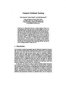
3.1 Network Model A DTN is an overlay network that is built upon underlying networks e.g. wireless ad hoc networks. Its network architecture is based on the asynchronous message (called bundle) forwarding paradigm presented in (K.Fall,2003). Only those nodes that implement the DTN functionalities e.g. sending, storing, and receiving bundles are considered DTN nodes, while the others are denoted as normal nodes. A DTN link may span several underlying links. Fig. 1 depicts a simple DTN example. In Figure 1, n3 and n4 are neighbors in the DTN layer but in the underlying network layer, this DTN link goes through two wireless hops (via n6 and n7 ). A DTN node j is considered a neighbor of another DTN node i only if there is an end-toend path connecting them in the underlying network. In this work, we assume the underlying network is ad hoc network and hence an ad hoc networking routing scheme like DSR (J. Broch et al, 1998) is used to find a route between any two DTN nodes.

DTN Layer

n5

n1

n8

S n10

n3

Underlying Network n2 n4

n9

n6 n7

DTN node Regular node

Physical Link DTN Link

Fig. 1. A simple DTN example

In the DTN layer, bundles are transmitted in a store-andforward manner hop by hop. This means that when a DTN node has unicast/multicast bundles to deliver, DTN

unicast/multicast routing scheme will be used. If a DTN node cannot find an available next-hop DTN node to deliver the bundles, then the bundles will be stored in its buffers. Each DTN node has finite-size buffers. To ensure reliable delivery, a custodian transfer feature has been proposed (K. Fall et al, 2003). When the custody transfer feature is turned on, a DTN node i will find another DTN node j which is willing to accept the custody of a particular bundle i.e. the other node is willing to accept the responsibility of delivering the bundle to its destination. Node i will send node j a custody request message and if node j is willing, node j will reply with a custody accept. The custody request message is piggybacked to the bundle that node i sends node j. Once node i receives such an acknowledgment, it can remove the sent bundle from its buffers. 3.2 Multicasting Model Multicast in DTNs is defined as the one-to-many or many-to-many bundle transmissions among a group of DTN nodes. A multicast source uses either a multicast end-point identifier descriptor (EID) e.g. *.cse.lehigh.edu, or an explicit list of the names of individual DTN multicast receivers as the destination address for multicast bundles. The later approach may not be scalable when the number of DTN multicast receivers grow large. Group Membership Management Several semantic models of DTN multicast membership have been studied in (W. Zhao et al, 2005). For example, in the temporal membership (TM) semantic model, each bundle includes a membership interval that specifies the period during which the group members are defined. If the membership interval of a bundle from a multicast group G is [t1,t2], it means that the intended receivers of the message consist of all members of the multicast group G at any time during [t1,t2]. Multicast messages can be delivered at any time. We adopt this TM model for our multicast work. A DTN node k can send the multicast source a Group_Join message with the start-time tsk and end-time tek. The multicast source can add this node’s membership information into a receiver list that it maintains. The membership information can be included in the bundles to be delivered or sent separately as control messages to nexthop custodians. The inclusion of membership information in the bundles works for small groups but separate control messages have to be used for large groups. The membership information allows each intermediate custodian, m, to check if the membership of a receiver, v, has expired. If a multicast bundle carries a list of valid receivers in its header, then node m will not include v’s identifier in the relayed bundle if v’s membership expires. If a multicast EID is used, then node m updates the information it maintains when it receives new membership information, and relays the bundle only if there is at least one active downstream receiver (i.e. a receiver whose membership has not expired). 4. MULTICASTING ROUTING APPROACHES FOR DTNS

4.1 Existing Multicasting Approaches

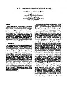
As we mentioned before, DTNs suffer from frequent network partitions. The dynamically changing network topology makes the maintenance of any multicast tree in DTNs challenging. The performances of different multicast approaches depend on how much current network information is available to the DTN nodes. Therefore, situational information needs to be collected and disseminated continuously so that new information can be used to adjust the message delivery paths. Such data collection and dissemination procedures incur overhead. Thus, a tradeoff between improving delivery performance and incurring extra overhead needs to be done. Various policies that utilize different amounts of situational information for routing decisions can be created for applications with varying quality of service requirements. An obvious multicast delivery approach is to let the source send a separate bundle to each of the receivers. Each duplicated bundle will be delivered to its intended receiver using the DTN unicast routing scheme. This is referred to as U-Multicast. This approach is wasteful since a DTN node may receive multiple copies of the message intended for different receivers. In addition, there are two existing approaches for supporting multicast communications in a DTN, namely DTBR and OS-Multicast. An illustrative example of these two approaches is shown in Fig.2. Note that the nodes shown in the Fig 2 are DTN nodes so nodes 1 and 3 may not be direct neighbors in the underlying network. We assume in this work that the underlying network is ad hoc network and hence an adhoc networking routing scheme like DSR is needed to find a route between any two DTN nodes. 0

0

1

1

2

4

3

5

(a)

3

2

6

4

5

(b)

6

Fig. 2. Multicast approaches in DTN (a) DTBR, (b) OS-multicast: when link 2
5 is unavailable and link 3 to 5 becomes available, node 3 will take advantage of the current available link immediately.

•

DTBR (W. Zhao et al, 2005): This is a dynamic treebased multicasting algorithm designed for DTNs. In DTBR, the upstream node will assign the receiver list for its downstream neighbors based on its local view of the network conditions. The downstream nodes are required to forward bundles only to the receivers in the list, even if a new path to another receiver (not in the list) is discovered. For example, in Figure 2(a), let say link 1-2 is unavailable when the multicast bundle reaches node 1. Then, node 1 will use node 3 to deliver to nodes 5 and 6 and store a copy of the bundle. Node 1 can send the stored bundle to node 2 when the link 12 becomes available again since this is the only route (via link 1-2) that node 1 knows of to reach node 4. DTBR assumes that each node has complete knowledge or the summary of the DTN link states in the network. However, this is hard to achieve in practical scenarios.

NODE DENSITY-BASED ADAPTIVE ROUTING SCHEME FOR DISRUPTION TOLERANT NETWORKS •

On-demand Situation-aware multicast (OSmulticast) (Q. Ye et al, 2006) Like the DTBR scheme, OS-multicast is also a dynamic tree-based multicast approach. A unique multicast tree is constructed for each bundle and the tree is adjusted at each intermediate DTN node according to the current network conditions. When a DTN node receives a bundle, it will dynamically adjust an initially constructed tree based on its current knowledge of the network conditions. Via such adjustments, any newly discovered path will be quickly utilized. For example, in Figure 2(b), the link between 2 and 5 is broken but when the bundle reaches node 3, node 3 knows that it can reach node 5 and 6. So, it will send a copy to both nodes 5 and 6. The downside of the OS-multicast approach is that a receiver may receive multiple copies Local Density Estimation Initialization: NN ← 0; LOCAL_DENSITY

//the number of 1-hop neighbors // 0 indicates low density, //1 indicates high density initialize(RESPONSE_TIMER); //waiting timer for the response from neighbors after broadcasting Neighbor Discovery packet NDp

← 0;

initialize(BROADCAST_TIMER); Neighbor_Discovery packet NDp activate(BROADCAST_TIMER); broadcast

//timer for broadcasting //activate the timer for 1st

Upon expiration of BROADCAST_TIMER do localDensityDetection(); Upon reception of NDp do NRp ← composeNeighborResponse( ); //compose Neighbor_Response packet; send(NRp); // Send the Neighbor_Response message to the sender of the Neighbor Discovery message Upon reception of NRp from a new neighbor node do NN ← NN +1; update two-hop neighbor table;

Two Hop Neighbor Contact Estimation Initialization: initialize(BROADCAST_TIMER);

//timer for broadcasting Neighbor_Discovery packet NDp activate(BROADCAST_TIMER); //activate the timer for the 1st broadcast initialize(AGE_TIMER); //aging timer activate(AGE_TIMER);

Upon expiration of BROADCAST_TIMER do Include CP[i][k] in NDp //CP[i][k] =contact probability to the node k

Procedure UpdateTwoHopNeighbor(NDp) For each CP[j][k] in NDp if CP[i][j]*CP[j][k]>CP[i][k] then CP[i][k]= CP[i][j]*CP[j][k] Upon expiration of AGE_TIMER do For each node CP[i][k] if no NDp received from node k then CP[i][k]= CP[i][k]* β

PROCEDURE localDensityDetection( ) NN ← 0; NDp ← composeNeighborDiscovery(); broadcast(NDp); activate(RESPONSE_TIMER);

Figure 3(b): Two-Hop Neighbor Contact Estimation

//compose

PROCEDURE composeNeighborResponse() //compose Neighbor_Response packet; create Neighbor_Response packet NRp; append 1-hop neighbor information (id, location, velocity) in NRp; append own identifier, location and velocity information in NRp packet;

of the same bundle.

(a) Local Node Density Estimation Each node periodically (e.g. every 20 ms) broadcasts a neighbor discovery packet using regular power transmission. On receiving a neighbor discovery packet, a node composes a neighbor response packet including this node’s information (e.g. identifier, location, and velocity) and this node’s 1-hop neighbor’s information (e.g. the neighbor’s identifier, location, and velocity) and sends the neighbor response packet to the originator of the a neighbor discovery packet after some random backoff delay. Thus, each node can estimate the number of neighbors it has periodically, denoted as Nd . If a node’s Nd drops below a threshold, K, during a neighbor discovery period, the node sets a sparsely connected flag. Figure 3(a) shows the pseudo code for the local node density estimation.

Upon reception of NDp from node j do Prob[i][j]=1; UpdateTwoHopNeighbor(NDp)

Upon expiration of RESPONSE_TIMER do if NN ≤ DENSITY_THRESHOLD then LOCAL_DENSITY ← 0; else LOCAL_DENSITY ← 1; activate(BROADCAST_TIMER);

PROCEDURE composeNeighborDiscovery() Neighbor_Discovery packet; create Neighbor_Discovery packet NDp; append own identifier in NDp; return NDp;

Figure 3(a): Local Node Density Estimation

4.2 Context Aware Multicast Routing (CAMR) Scheme In this section, we describe the CAMR scheme we proposed. The CAMR scheme consists of five components: (a) Local Node Density Estimation, (b) 2-Hop Neighbor Contact Probability Estimate, (c) Route Discovery, (d) Route Repair and (e) Data Delivery. The pseudo codes for the CAMR scheme are shown in Figure 3.

(b) 2-hop Neighbor Contact Estimation Each node also maintains its contact probabilities with its 2hop neighbors. The contact probability of a neighbor is set to 1 as long as a node, ni , can receive neighbor response messages from a neighbor, nj , periodically. When ni fails to hear a neighbor response message from nj, then ni decreases its contact probability with nj by a factor of β periodically (since the neighbor discovery message is sent out periodically). Rather than immediately reducing the contact probability to zero, the aging factor, β , is used to avoid the ping-pong effect (i.e. a node may move in and out of the transmission range frequently). These contact probabilities

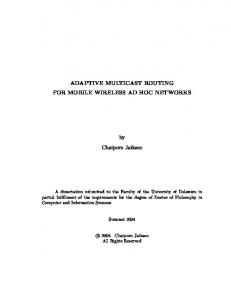
allow a node to send the messages directly without incurring the route discovery overhead if the destination happens to be within its 2-hop neighbourhood. (c) Route Discovery A source initiates a route discovery process if it cannot reach any of the receivers to which the multicast traffic needs to be delivered. Before any intermediate node rebroadcasts a route request message it receives, it first checks to see if its sparsely connected flag is set. If the flag is set, then the node rebroadcasts the route request message using high power transmission (e.g. at a level that results in a transmission range of 375m or 500m). Otherwise, the intermediate node re-broadcasts the route request using regular power. Any node that receives a high power route request will make a note since that node needs to issue a high power route reply when it hears a response back from a downstream node. n8

S

n7

R7

R6

n1 n2

n3

R8

n4 n5

n6

R5 R1

n9 n11

n10

R4 R2

R3

Fig. 4. CAMR scheme

Assume that S is the multicast source and there are eight multicast receivers as shown in Figure 4. S knows it can reach R6 using its 2-hop neighborhood information so S does not need to issue any route request for R6. The route request issued by S for the other seven receivers is flooded by intermediate nodes using regular power until it reaches node R6 and n3. R6 and n3 will re-broadcast the route request using high power since their observed local node densities drop below the threshold K. When the route request eventually reaches any intended multicast receiver, it will issue a route reply. Through this process, S can eventually construct a merged multicast delivery tree after hearing route replies from downstream nodes for all the eight receivers. Note that this multicast tree is not static as in wired multicast or static wireless mesh network scenario. Note further that the location and velocity information of the nodes sending route request and route reply messages are piggybacked. For example, when R6 receives a route reply from n4, R6 will record the location and velocity information of n4 and that n4 is the next hop node for delivering bundles from this multicast session. Later, when S sends multicast bundles, S will piggyback a multicast receiver list in all multicast bundles that are sent out. Thus, R6 knows that it is responsible for delivering the multicast messages to R1, R5, R7 and R8. Upon receiving the multicast bundles, R6 travels closer to n4 so that the multicast bundles can be delivered using regular power transmission. Since the location and velocity information is included in the route reply from n4 to R6, R6 can estimate where it can reach n4 with regular power transmission. Note

that R6 may decide to travel towards n4 only after receiving multiple multicast bundles (aka batch delivery). Similar actions are taken by n3 to deliver multicast bundles to n6. Figure 3(c) shows the pseudo code for our route discovery process. There are several optimizations that one can make e.g. the source can flood a multicast route request where the identifiers of all receivers are included rather than sending individual route request, the intermediate nodes can merge the route replies from different downstream nodes that can reach different multicast receivers. In this paper, our simulation study does not include these optimizations. (d) Route Repair In CAMR, one can use local route repairs when the multicast tree is broken as a result of node mobility. Let us assume that when multicast bundles arrive at node n4 in Figure 4, n9 moves away. There are two ways whereby n4 can repair the route: (a) n4 can issue a route request to find a route to R8, or (b) n4 can make use of the location and velocity information to travel closer to n9 and not incur extra route discovery messages for local repair. We refer to the version where n4 issues a route request message to perform the local route repair as CAMR-I and the version where n4 uses the location and velocity information to perform route repair as CAMR-II. The CAMR-II scheme will incur smaller routing overhead than the CAMR-I scheme. Figure 3(d) shows the pseudo code for our route repair procedure. (e) Data Delivery For data delivery, an extra header is piggybacked to each data bundle. The header contains information on the identifiers of the receivers to which a particular multicast bundle needs to be delivered. Any intermediate node that supports CAMR scheme will duplicate the bundle if the node discovers that it is the branching point. A node acts as a message ferry during data delivery if it uses a high power route request to reach a downstream node. Such a node will only move as a message ferry after accumulating enough bundles (the threshold is denoted as MOVING_THRESHOLD). The ferrying node travels towards the last known position of the next-hop DTN node. If the ferrying node hears the beacons from this next-hop DTN node, then it can transfer all the accumulated bundles destined for this next hop node. Since the down-stream next hop node may have already moved by the time a ferrying node moves, this ferrying node may not find that next-hop node. In that case, this ferrying node will return to its original position and perform a route rediscovery for the receivers that it needs to reach. Custodian transfer feature (K. Fall et al, 2003) is turned on in our CAMR scheme. This means that after a node ni receives a custodian acknowledgment from a downstream node,

n j , ni can

remove the acknowledged bundle from its storage.

NODE DENSITY-BASED ADAPTIVE ROUTING SCHEME FOR DISRUPTION TOLERANT NETWORKS

Route Discovery Process Upon reception of route request for data packet delivery do RDp=composeRouteDiscovery(); //compose route discovery(RDp) packet if LOCAL_DENSITY ==0 then broadcast RDp with high transmission power; else broadcast RDp with regular transmission power; Upon reception of RDp do if RDp is duplicate drop RDp; return; else RDp’ RDp //prepare new route discovery packet(RDp’) if lookUpReceiver( RDp)= =TRUE then RRp ← composeRouteReply(RDp’); forwardRouteReply(RRp); if LOCAL_DENSITY ==0 then node.id ← LOCAL_ID ; //indicates high node.power ← 1 ; power transmission is used RDp.forward_list ← RDp.forward_list ∪ node; //append current node to forward list rebroadcast RDp with high transmission power; else node.id ← LOCAL_ID ; node.power ← 0 ; //indicates regular power transmission is used RDp.forward_list ← RDp.forward_list ∪ node; rebroadcast RDp with regular transmission power; Upon reception of RRp do if RRp.destination= = LOCAL_ID then route  reverse(RRp.reply_list); //forwarding route is the reverse of the reply route merge route to multicast_tree; use multicast_tree to deliver data packets in buffer else forwardRouteReply(RRp); PROCEDURE lookUpReceiver(RDp’) //see if receivers in the RDp’.receiver_list are in this node’s 2-hop neighbor table; if found receivers then append nodes to the destination to RDp.forward_list; return TRUE; else return FALSE; PROCEDURE composeRouteReply(RDp’) create Route_Reply packet RRp; RRp.destination ← RDp’.source; RRp.reply_list ← reverse(RDp’.forward_list); //Reply route is the reverse of the discovered route return RRp; PROCEDURE composeRouteDiscovery() Create Route_Discovery packet RDp;

Figure 3(c) Pseudo Code for Route Discovery

Route Repair Upon loss of acknowledgment from the next_hop along the data route do routeRepair(next_hop); PROCEDURE routeRepair(next_hop) CAMR-I: RDp composeRouteDiscovery(); if LOCAL_DENSITY==0 then broadcast RDp with high transmission power; else broadcast RDp with regular transmission power; CAMR-II: if lookUpLocation(next_hop) ==TRUE then move close to the estimated next_hop.position; else goto CAMR-I; PROCEDURE lookUpLocation(next_hop) next_hop.position check old location and velocity of next_hop in neighbor table and estimate current location of next_hop distance 

next _ hop. position − my. position

;

if distance > THRESHOLD then //if distance is too long, give up and return FALSE; //use CAMR-I scheme else return TRUE;

Figure 3(d): Pseudo Code for Route Repair

5.

PERFORMANCE EVALUATION

5.1 Simulation Set Up To evaluate the performance of different multicast algorithms, we implemented U-multicast, OS-multicast, DTBR, and CAMR (only version II) in the ns2 simulator. The performance metrics that are used to compare different multicast routing approaches are: i) message delivery ratio (DR), which is defined as the number of unique multicast packets which successfully arrive at all the receivers over the total number of packets which are expected to be received, e.g. if the source sends out N packets with R receivers and each receiver receives xi packets, then DR =

∑x

i

N *R

;

ii) data efficiency, which is the ratio between the number of unique multicast packets successfully delivered to the receivers, and the total data traffic generated in the networks; iii) overall efficiency, which is the ratio between the number of unique multicast packets successfully delivered to the receivers, and the total traffic generated (both data and control packets) in the networks; and iv) average message delay, which is the average of the end-to-end bundle delivery latencies for each algorithm (we observe similar delay performance results when we use the metric of median delay). Note that for the overall efficiency computation, we assume that the power required to transmit a data packet is a

linear function of the packet size. In addition, we assume that a route request or route reply message is 35 bytes long. Each route request or reply message that is transmitted at high power is counted as (k= (

r2 4 ) ) times that of a route r1

request/reply message that is transmitted at regular power where r2 and r1 is the transmission range (TR) of the high and regular power transmission respectively e.g. k=16 when the high power transmission range is 500 m but the regular power transmission range is 250m. The neighbor discovery interval is set at 10 seconds, and β is set at 0.8 in all our experiments unless otherwise stated. In our experiments, unless otherwise stated, we use a network with 40 nodes deployed randomly in a geographical 2

area of size 4000x4000 m . All nodes are DTN nodes unless otherwise stated. DSR is used as the routing approach for the underlying ad hoc networks for U-Multicast, DTBR and OS-Multicast schemes. And situational awareness is achieved through the communication between the DTN multicasting agent and the DSR routing agent. For CAMR, unless otherwise stated, the speed of the nodes not acting as message ferry is chosen uniformly between 1 m/s and 5 m/s. When a node acts as a message ferry, it moves with a speed of 15 m/s. The MAC layer is IEEE 802.11 with radio transmission range that varies from 250 m to 500 m. Table 1 summarizes the default simulation parameter values used. For each simulation run, we generate traffic for 1000 seconds and run the simulation for 10,000 seconds. Each data point is the average results obtained from at least 5 runs. Mobility Models In this work, we use three mobility models, namely (a) random waypoint (RWP) model, (b) Zebranet (Y.Wang et al ,2005) model, and (c) UMassBusNet (X. Zhang et al, 2007) model. In the RWP model, each node selects a randomly located destination and move towards that destination with constant speed. Once it reaches the destination, it pauses for a certain period of time before repeating the process again. The speed of the nodes not acting as message ferry is chosen uniformly between 1 m/s and 5 m/s. For the Zebranet model, we create a semi-synthetic Zebranet mobility model as follows: we synthesize node speed and turn angle distributions from the observed data and create other node-movements using the same distribution. We use both distance and time scaling to fit the original data found in the trace into the network environment that we are interested in. For the UMassBusNet model, we extract the locations of twenty buses at different times in one trace, and scale their relative locations to fit into the geographical area of interest. We first evaluate the sensitivity of the delivery performance of our CAMR scheme when certain tunable parameters e.g. high power transmission range, β are varied. Then, we compare the CAMR scheme with other DTN multicast schemes e.g. U-Multicast, DTBR (W. Zhao et al, 2005) and DTBR (Q. Ye et al, 2006). Next, we study the delivery

performance of CAMR in different scenarios e.g. varying number of groups, varying group size, different mobility models. Table 1 Simulation Parameters Parameter Value Simulation area 1000x1000, 2000x2000, 3000x3000, 4000x4000m2 Simulation time 10000 seconds Buffer Size 600 messages 10 sec/0.8 ND Interval/β High Power TR Default:500m MovingThreshold 10 (CAMR) Traffic pattern Default: 1 group 12 receivers Multicast source generates CBR traffic with a packet size of 512 byte Mobility model Default: RWP with (vmin=1m/s, vmax=5m/s) Others: Zebranet, UMassBusNet 5.2 Sensitivity Analysis of Parameters in CAMR 5.2.1 Impact of Transmission Range

First, we evaluate the difference in the delivery performance when the high power transmission range is set either to 375m or 500m. We use one multicast group with one source and 12 receivers. The multicast source generates traffic at a rate of 1 pkt/s. Tables 2 tabulate the delivery ratio, average delay, and the data efficiency results that we obtain when the high power transmission range is set to either 375m or 500m respectively. The delivery ratio achieved using a high power transmission range of 500m is slightly better than using 375m. The average delay with 500m is also smaller. Thus, we use 500m as the high power transmission range for the rest of our study in this paper. Aging Factor

Delivery Ratio

Average Delay (s)

1000x1000

375m 0.93

500m 0.93

375m 81

500m 81

2000x2000

0.89

0.90

2421

2327

3000x3000

0.82

0.85

2845

2700

4000x4000

0.75

0.80

3953

3725

Data Efficiency& Overall Efficiency 375m 500m 0.40/ 0.18 0.37/ 0.16 0.31/ 0.14 0.28/ 0.12

0.40/ 0.18 0.36/ 0.14 0.31/ 0.11 0.27/ 0.10

Table 2: Results using High Power Tx Range of 375/500 m. 5.2.2 Impact of different neighbor discovery interval and aging factor values.

We conduct a set of experiments to investigate the impact of using different values for the neighbor discovery (ND) interval with the 40 nodes over 4000x4000m2 network scenario. We use a single multicast group with 12 receivers and the multicast source generates packets at rate of 1 pkt/s. The results are tabulated in Table 3(a). With an interval of 10 seconds, the delivery ratio is 80% but with 20 seconds, it drops to 74%. When the neighbor discovery interval is longer, the nodes make routing decisions based on older

NODE DENSITY-BASED ADAPTIVE ROUTING SCHEME FOR DISRUPTION TOLERANT NETWORKS information and hence the delivery performance suffers. We will use a neighbor discovery interval of 10 seconds for the rest of our paper.

believe that our CAMR scheme is the best choice for multicast delivery especially when the networks are very sparse e.g. with only 0.5 neighbor within its transmission range.

We also conduct a study on the impact of different aging factors on the data delivery performance. The results are tabulated in Table 3(b). The paired t-tests (Navidi 2006) show that the difference in the observed results is not statistically significant. This means that the delivery performance remains relatively the same when the β value lies within the range (0.4,0.8). Thus, we decide to use β =0.8 for the rest of our paper. ND Interval (sec) 10 15 20

Delivery Ratio 0.80 0.76 0.74

Average Delay (s) 3725 3852 4122

Data Efficiency

Overall Efficiency

0.27 0.26 0.28

0.1 0.1 0.1

Figure 5(a) Delivery Ratio using RWP mobility model

Table 3(a): Results with different neighbor discovery intervals

Aging Factor 0.4 0.6 0.8

Delivery Ratio 0.83 0.81 0.81

Average Delay(s) 3628 3673 3725

Data Efficiency 0.27 0.27 0.27

Overall Efficiency 0.1 0.1 0.1

Table 3(b): Results with different aging factors

5.3 Comparison with Other Multicast Routing Approaches In this section, we compare the CAMR scheme with UMulticast, DTBR and OS-Multicast schemes using the random waypoint mobility model with 40 nodes distributed in an area which ranges from 1000x1000 m2 to 4000x4000m2 . A single multicast group with 12 receivers is used in this set of experiments. The multicast source generates packets at a rate of 0.5 pkt/s. Fig 5(a),5(b), and 5(c) plot the delivery ratio, the average delay and the data efficiencies of the different schemes. From the plots, we see that CAMR achieves the highest delivery ratio (see Fig 5(a)) with similar delay performance. The price to pay is a slight decrease in data efficiency (see Fig 5(c)). The average delay in CAMR may look larger (see Fig 5(b)) because of a longer tail in the delivery latency distribution. However, if we consider only those packets that are successfully delivered in all schemes, the average delay achieved by CAMR is smaller e.g. DTBR can only achieve 9.7% delivery ratio in the 40 nodes by 3000x3000 m2 scenario and has an average delay of 1460 seconds and a data efficiency of 0.145. Using CAMR, the average delay of similar packets is about 129 seconds with a data efficiency of 0.39. We expect that the CAMR scheme will outperform all other schemes when the network becomes very sparse. Since store-and-forward approach is not used for real time traffic but to ensure that many messages can be delivered even in scenarios where no end-to-end paths exist, we

Figure 5(b) Average Delay using RWP mobility model

Figure 5(c) Data Efficiency using RWP mobility model 5.4 Impact of Mobility Models

In this section, we investigate the impact of mobility models on the delivery performance of the CAMR scheme. We use the default network scenario with 40 nodes distributed over 4000x4000m2. The nodes move according to either the (a) RWP, (b) Zebranet, or (c) UMassBusNet model. We use a multicast group with 12 receivers. The packet rate generated by the multicast source is varied from 0.25 pkt/s to 2 pkt/s. Figures 6(a),6(b), and 6(c) plot the delivery ratio, the average delay, and the data efficiency results that we obtain.

better delivery performance. When nodes are in different clusters, it is difficult to find a relaying node that can help to transfer packets between these two clusters.

Figure 6(a): Delivery Ratio vs Packet Rate

The delivery performance using the Zebranet model is better than that using the RWP model because the nodes in the Zebranet model move faster (the average node speed is 6 m/s in Zebranet model but only 3 m/s in the RWP model). The mean intercontact time and the contact duration between any two nodes are shorter in the Zebranet model. However, the contact duration in the Zebranet model is long enough to allow nodes to transfer queued packets to other nodes during their encounters. With shorter intercontact time, packets will be queued shorter. Thus, the delivery ratio is higher in the Zebranet model. The data efficiency is the best using the UMassBusNet model because the average number of hops of successfully delivered packets in this model is 2.1. Those packets that require more hops are dropped. The average number of hops taken to deliver packets using the Zebranet model is 2.6 (faster node speed in the Zebranet model results in shorter path) while that for the RWP model is 3. That explains why the data efficiency for the Zebranet model is higher than that for the RWP model. 5.5 Impact of different number of multicast groups

Figure 6(b): Average Delay vs Packet Rate

Figure 6(c): Data Efficiency vs Packet Rate

From the plots, we can draw a few conclusions. Among the three mobility models, the UMassBusNet model results in the poorest delivery performance. The paired t-test results did show that the difference in the delivery ratio between RWP/Zebranet and UMassBusNet is significant (with a P value < 0.008). The poorer delivery performance in the UMassBusNet model is due to two factors, namely (i) the mean intercontact time in UMsasBusNet model is longer and its mean contact duration is shorter. This means fewer packets can be transferred when two nodes encounter each other and that packets need to be queued longer and hence have high probability of being dropped as a result of buffer overflows, (ii) the nodes move in different clusters. Those nodes (buses) that move using similar routes are in one cluster and packets transferred between these nodes have

In this section, we investigate the impact of different number of multicast groups on the delivery performance of the CAMR scheme. We use the default network scenario with 40 nodes distributed over the 4000x4000m2. The nodes are allowed to move according to either the RWP or the UMassBusNet models. Each group has 6 receivers randomly chosen from the 40 nodes. Each multicast source generates packets at a rate of 1 pkt/s. We vary the number of multicast groups from 1 to 6. Figures 7(a),7(b) and 7(c) plots the delivery ratio, the average delay and the data efficiency results that we obtain. There are several observations we made from the results. First, the delivery performance of the CAMR scheme degrades slowly with increasing number of groups and hence it shows that the scheme is scalable. Second, as the number of groups increases beyond 4 groups, the delivery ratio degrades faster. With both mobility models, the delivery ratio drops only by 8-10% as the number of groups increases from one to four but drops by 16% as the number of groups increases from four to six. Such degradation is due to buffer overflows since the total packets each node needs to store increases with more groups. About 20% of the nodes reach their buffer limitation in scenarios with more than 4 groups. With the RWP model, the average delay only increases by 16.9% as the number of groups increases from one to six. However, with the UMassBusNet model, the average delay increases by 36% as the number of groups increases from one to six groups. The larger increase is expected since the nodes in the UmassBusNet model move according to certain clusters (nodes that take the same route belong to one cluster) and hence there are more network partitions. The delivery latency for packets that

NODE DENSITY-BASED ADAPTIVE ROUTING SCHEME FOR DISRUPTION TOLERANT NETWORKS need to be delivered between nodes in different clusters will be larger.

Figure 7(a): Delivery Ratio vs # of Groups

all nodes support DTN functionalities. We use one multicast group with 12 receivers where the multicast source generates packets at a rate of 1 pkt/s. We compare the case where 50% of the nodes are DTN nodes with the case where all nodes are DTN nodes. Table 4 tabulates our results for different network scenarios. From Table 4, we see that with only 50% of the nodes being the DTN nodes, the delivery ratio drops by 10% in the 2000x2000m2 scenario but it drops by 14% to 16% when the network becomes very sparse (for the 3000x3000m2 and 4000x4000m2 scenarios). With fewer nodes that support DTN functionalities, there are fewer chances of using message ferrying to deliver packets across partitioned networks. Therefore, the delivery ratio is poorer with 50% of the nodes being the DTN nodes. The average delay drops with fewer nodes supporting DTN functionality. Such a drop is misleading because packets that are more difficult to be delivered are being dropped in the 50% DTN nodes scenario but are delivered (with much higher delay) when all nodes support DTN functionality. The data efficiency is only slightly worse with 50% nodes supporting DTN functionality. This is due to the increasing number of retransmissions when only 50% of the nodes support DTN functionality. Table 4 Impact of having different percentage of nodes supporting DTN functionalities Simulation Area

Delivery Ratio

Average Delay (s)

1000x1000

50% 0.93

100% 0.93

50% 81

100% 81

2000x2000

0.81

0.90

2256

2327

3000x3000

0.73

0.85

2567

2700

4000x4000

0.67

0.80

3613

3725

Figure 7(b): Average Delay vs # of Groups

Data Efficiency& Overall Efficiency 50% 100% 0.40/ 0.40/ 0.18 0.18 0.34/ 0.36/ 0.14 0.14 0.31/ 0.31/ 0.11 0.11 0.24/ 0.27/ 0.10 0.10

5.7 Impact of Different Maximum Node Speeds.

Figure 7(c): Data Efficiency vs # of Groups Third, we observe as before that the delivery performance using UMassBusNet model is poorer than that with the RWP model. This poorer performance is due to two factors: (i) the mean intercontact time for the UMassBusNet trace is longer, and (ii) nodes in the UMassBusNet model move according to certain routes and hence there are more network partitions in the UMassBusNet model than in the RWP model. As discussed before, the data efficiency with the UMassBusNet model is higher than that with the RWP model because only those packets that require fewer hops are successfully delivered in the UMassBusNet model. The average number of hops is 2.1 for the UMassBusNet model but 3 for the RWP model. 5.6 Impact of different percentage of DTN nodes

In some scenarios, not all nodes may support DTN functionalities. Nodes that do not support DTN functionalities can not be message ferries. Thus, in this section, we investigate the performance difference when not

In this section, we explore how the different (vmin, vmax) values affect the data delivery performance. We use two network scenarios: 40 nodes distributed over (i) 4000x4000m2 and (ii) 3000x3000m2. One multicast group with 12 receivers is used. The multicast source generates packets at a rate of 1 pkt/s. The multicast receivers are randomly chosen among the 40 nodes. Figures 8(a), 8(b), and 8(c) plot the delivery ratio, average delay and data efficiency for the different (vmin , vmax ) values. From the results, we can see that the delivery ratio increases slightly initially with increasing node speeds but the average delay decreases significantly with increasing node speed. As a node moves around faster, it encounters more nodes and hence is able to disseminate messages better. As a result, the average delay decreases due to shorter mean intercontact time. However, the contact duration will become shorter too with increasing node speed. As long as the contact duration is long enough to allow nodes to transfer queued packets when they meet one another, the delivery ratio will not degrade but may improve (since the same forwarding node can be used for multiple packets).

UMassBusNet mobility model results in the poorest delivery performance due to its large intercontact time. We hope to implement the CAMR scheme in a DTN testbed for empirical evaluations. ACKNOWLEDGEMENT

This work is sponsored by Defense Advanced Research Projects Agency (DARPA) under contract W15P7T-05-C-P413. Any opinions, findings, and conclusions or recommendations expressed in this material are those of the authors and do not necessarily reflect the views of DARPA. This document is approved for public release, unlimited distribution. Figure 8(a): Delivery Ratio vs Node Speed REFERENCES

Figure 8(b): Average Delay vs Node Speed

Figure 8(c): Data Efficiency vs Node Speed

6.

CONCLUSION

In this paper, we have developed a context-aware adaptive multicast routing scheme for DTNs. Our scheme is flexible and can adapt to different network environments e.g. different node densities, different mobility models. We have evaluated our CAMR scheme and compare it with other existing proposed multicast routing schemes for DTNs. Our results show that the CAMR scheme is more flexible and can provide the highest delivery ratio with lower average delay (comparing only those common packets that are delivered in all schemes) especially when the network becomes sparser. Via simulation studies, we also have shown that CAMR scales well with increasing number of groups and maintains a high delivery ratio even with increasing node speed. We also have shown that the

S. Bae, S. J. Lee, W. Su, and M. Gerla, “The design, implementation, and performance evaluation of the ondemand multicast routing protocol in multihop wireless networks”, IEEE Network, pp 70-77, January, 2000. J. Broch et al, “A performance comparison of multihop wireless adhoc network routing protocol”, Proceedings of Mobicom, 1998. S. Burleigh, A. Hooke, L. Torgeson, K. Fall, V. Cerf, B. Durst, K. Scott, and H. Weiss, “Delay tolerant networking – an approach to interplanetary internet”, IEEE Communications Magazine, June, 2003. J. Burgess, B. Gallagher, D. Jensen, B.N. Levine, “MaxProp: Routing for Vehicle-Based DisruptionTolerant Networking”, to appear in Proceedings of IEEE Infocom, April, 2006. V. Cerf et al, “Delay-Tolerant Network Architecture”, Internet Draft, draft-irtf-dtnrg-arch-02.txt, July 2004. A. Cerpa, J. Elson, D. Estrin, L. Girod, M. Hamilton, J. Zhao, “Habitat monitoring : application driver for wirelss communications technology”, Proceedings of ACM Sigcomm Workshop on Data Communications, April, 2001. M. Chuah, L. Cheng, and B. D. Davison, “Enhanced Disruption and Fault Tolerant Network Architecture for Bundle Delivery (EDIFY)”, Proceedings of IEEE Globecom, 2005 K. Fall, “A delay-tolerant network architecture for challenged Internets”, Proceedings of SIGCOMM’03, August 2003. K. Fall, W. Hong and S. Madden, “Custody transfer for reliable delivery in delay tolerant networks”, IRB-TR-03030, July 2003. K. Fall, “Messaging in difficult environments”, Intel Research Berkeley, IRB-TR-04-019, Decemeber, 2004. S. Jain, K. Fall, and R. Patra, “Routing in a delay tolerant networking”, Proceedings of ACM Sigcomm, August/September, 2004. S. Jain, M. Demmer, R. Patra, and K. Fall, “Using Redundancy to cope with Failures in a Delay Tolerant Network”, Proceedings of Sigcomm 2005. R. Malladi, and D. P. Agrawal, “Curent and future applications of mobile and wireless networks”,

NODE DENSITY-BASED ADAPTIVE ROUTING SCHEME FOR DISRUPTION TOLERANT NETWORKS Communications of the ACM, Vol 45, pp 144-146, 2002. A. Lindgren, A. Doria, O. Schelen, ”Probabilistic routing in intermittently connected networks”, Sigmobile, Mobile Computing and Communications Review, Vol 7(3), pp 19-20, 2003. J. Moy, “Multicast extension to OSPF”, IETF RFC 1584, 1994. W. Navidi, “Statistics for Engineers and Scientists”, McGraw Hill, 2006. T. Spyropoulos, K. Psounis, and C. S. Raghavendra, “Spray and Wait:An efficient routing scheme for intermittently connected mobile networks”, Proceedings of ACM Sigcomm Workshop on Wireless Delay Toelerant Networks (WDTN), August 2005. Y. Wang, et al, “Erasure-Coding Based Routing for Opportunistic Networks”, Proceedings of Sigcom WDTN workshop, August, 2005. D. Waitzman, C. Patridge, and S. Deering,”Distance Vector Multicast Routing Protocol (DVMRP)”, IETF RFC 1075, 1988. J. Wu, S. Yang, and F. Dai, “Logarithmic Store-CarryForward Routing in Mobile Ad Hoc Networks”, IEEE Transmaction on Parallel and Distributed System, June, 2007 J. Xie, R. R. Talpade, A. Mcauley, and M. Y. Liu, “AMRoute: ad hoc multicast routing protocol”, Mobile Networks and Applications, Vol 7, Issue 6, pp 429-439, 2002. Q.Ye, L. Cheng, M. Chuah, and B. D. Davison, “OnDemand Situation Aware Multicasting in DTNs”, Proceedings of IEEE VTC, Spring, 2006. X. Zhang, J. Kurose, B Levine, D. Towlsely, and H. Zhang, “Modeling of a bus-based disruption tolerant network trace”, Proceedings of ACM Mobihoc, Sept, 2007. Z. Zhang, Q. Zhang, “Delay/Disruption Tolerant Mobile Ad Hoc Networks: Latest Developments”, Wireless Communications and Mobile Computing, May 2007. W. Zhao, M. Ammar, and E. Zegura, “A message ferrying approach for data delivery in sparse mobile adhoc networks”,Proceedings of ACM Mobihoc, May, 2004. W. Zhao, M. Ammar, and E. Zegura, “Multicasting in delay tolerant networks: semantic models and routing algorithms”, Proceedings of ACM Sigcomm Workshop in DTN, August, 2005.

WEBSITES

DARPA Disruption Tolerant Networks Program http://www.darpa.mil/ato/solicit/dtn/ , accessed on August 3rd, 2005. UCB/LBNL/VINT, “The Network Simulator ns-2”, Online at http://www.isi.edu/nsnam/ns/