WSEAS TRANSACTIONS on SYSTEMS and CONTROL
Patricia Grof, Peter Baranyi, Peter Korondi
Convex hull manipulation based control performance optimisation PATRÍCIA GRÓF*,***, PÉTER BARANYI*,** and PÉTER KORONDI*,*** *Computer and Automation Research Institute/Cognitive Informatics Research, Budapest, Hungary **Budapest University of Technology and Economics/Dept. of Telecommunications and Media Informatics, Budapest, Hungary *** Budapest University of Technology and Economics/Dept. of Mechatronics, Optics and Engineering Informatics, Budapest, Hungary
[email protected],
[email protected],
[email protected] Abstract: - This paper deals with the topic of qLPV state-space model based control design in which LMIs are used to optimize the multi-objective control performance. In this paper we investigate how the manipulation convex hull of the polytopic model influences the control performance which is derived by LMIs. We examine these influences through the control design of the two dimensional aeroelastic system’s example. First we define various TP type polytopic model representations of a wing section whose vertices define different convex hulls. In the second step we investigate how these models lead to different control performances.
Key-Words: - polytopic model, TP model, LMI, convex hull shown that that global stabilization can be achieved by applying an additional control surface (e.g., in [15]). Adaptive-feedback linearization and global-feedbacklinearization techniques were introduced for two control actuators in [11] and the Ricatti-equation based method was used in [18]. Neural network based design was also discussed in [17]. Time delays are inevitable in control loops [18]. Time delay effects were introduced by Marzocca [19] and Yu et al. [20] focused on time delay feedback control of supersonic lifting surface on flutter boundary. Zhao [18] presented a systematic study on aeroelastic stability with single or multiple time delays in the feedback control loop. Tensor Product (TP) type polytopic model based state feedback, output feedback and LMI based controller design was proposed in [21, 22]. In [25] the effect of the convex hull manipulation of the TP models on the control performance is discussed. We proved that in modern LMI based multi objective control design the optimization of the control performance must include the manipulation of the convex hull beside constructing LMIs, and the TP model transformation offers a systematic solution. We can see some examples in [2629, 31 33] where TP model transformation is applied. In this paper we show that the manipulation of the convex hull is necessary for the the LMI based controller and observer design.
1 Introduction In the past few years various studies of aeroelastic systems have emerged. Regarding their properties one can find the studies of free-play nonlinearity by Price at al. in[2] and by Lee and LeBlanc [3] as well as a complete study of a class of nonlinearities [4]. O’Neil and Straganac[5] examined the continuous structural nonlinearity of these systems. Recent analysis is given in [6]. These papers conclude that an aeroelastic system may exhibit nonlinear phenomena such as limit cycle oscillation, flutter and even chaotic vibrations. Control strategies have also been derived for aeroelastic systems. Block and Straganac[7] show that in the case of large amplitude limit cycle oscillation behavior the linear-control methodologies do not stabilize these system consistently. At the NASA Langley research center a benchmark active control technique (BACT) wind tunnel model has been designed and control algorithms for flutter suspension have been developed by Waszak[8], Mukhopadhyay[9] and Keller and Joshi[10]. For an aeroelastic apparatus, tests have been performed in a wind tunnel to examine the effect of nonlinear structural stiffness, and control systems have been designed using linear control theory, feedback linearization techniques and adaptive control strategies.[11-12] One can find studies focusing attention on the two dimensional prototypical aeroelastic wing section. Block and Straganac[8] and Ko et et al.[13] proposed nonlinear feedback control methodologies for a class of non linear structural effects of the prototypical aeroelastic wing section. In this regard Ko et al. [11] developed a controller via partial-feedback linearization. It has been
ISSN: 1991-8763
2 Nomenclature a
691
= nondimensional distance from the midchord to the elastic axis;
Issue 8, Volume 5, August 2010
WSEAS TRANSACTIONS on SYSTEMS and CONTROL
Patricia Grof, Peter Baranyi, Peter Korondi
b
= semichord of the wing;
Ch clα
= plunge structural damping coefficient; = lift coefficients per angle of attack;
clβ
= lift coefficients per control surface deflection;
c mα
= moment coefficients per angle of attack;
c mβ
where S(p(t )) is a parameter varying object, and p(t ) ∈ Ω is time varying N dimensional parameter vector, where Ω = [a1 b1 ]× [a 2 b2 ] × ... × [a N bN ] ⊂ ℜ N is a closed hypercube. Parameter p(t ) can also include some elements of , in this case (2) is termed as quasi LPV (qLPV) model. Therefore this type of model is considered to belong to the class of non-linear models. Let us assume, that the size of S(p(t )) is O times I. Definition 2 (Finite element polytopic model):
= moment coefficients per control surface deflection;
cα h
= pitch-structural damping coefficient; = plunging displacement;
Iα
= mass moment of inertia;
kh
= plunge structural spring constant;
kα (α ) L M
m U xα
α β
ρ a,b,... a,b,... A, B,... A,B...
R
S( p ( t )) = ∑ w r (p(t )) ⋅S r
where p(t ) ∈ Ω . S(p(t )) is given for any parameter vector p(t )
as the parameter varying combinations of linear time invariant (LTI) system matrices S r ∈ R ( m + k )×( m + l ) also called LTI vertex systems. The combination is defined by the weighting functions wr ( p(t )) ∈ [0,1] . By finite we mean that R is bounded. The TP model belongs to the class of polytopic models. In case of the TP model the multi variable weighting functions wr ( p ) are decomposed to the product of one variable weighing functions wn ( pn ) . Definition 3 (Finite element TP type polytopic model):
= nonlinear stiffness contribution; = aerodynamic force; = aerodynamic moment; = mass of the wing; = free stream velocity; = nondimensional distance between the elastic axis and the center of mass; = pitching displacement; = control surface deflection; = the density of the air; = scalar values; = vectors; = matrices; = tensors
I1
S(p(t )) =
IN
I2
∑∑ ∑w ...
i1 =1 i2 =1
i N =1
= multiple product as A×1U1×2U2×3…×N UN;
N
(4)
(5)
contains one variable and continuous weighting functions wn ,in ( p n (t )) ∈ [0,1] , (in = 1...I N ) .(4)
Remark 1: TP model (5) is a special class of polytopic models (2), where the weighting functions are decomposed to the Tensor Product of one variable functions. For Linear Matrix Inequality based design, the convexity of the TP model is required. Therefore let us define the following types of TP models: Definition 4 (Convex type TP model): The TP model is convex if the weighting functions satisfy the following criteria:
The following definition are used in this paper: Definition 1 (qLPV model): Consider the Linear Parameter Varying State Space model: (1)
where u(t) is the input, y(t) is the output. The system matrix applying the state space model:
ISSN: 1991-8763
1, 2
where the (N+2) dimensional coefficient tensor S ∈ R I1 × I 2 ×...×I N ×( m + k )×( m +l ) is constructed from the LTI vertex systems S i1,i2 ...iN (4) and the row vector w n ( pn (t )) ∈ [0,1]
3.1 Concept of TP type polytopic model
A (p(t )) B(p(t )) S(p(t )) = C(p(t )) D(p(t ))
( pn (t )) ⋅ S i i ...i
,
Tensor Product model transformation
x& (t ) = A (p(t ))x (t ) + B(p(t ))u(t ) y (t ) = C(p(t ))x (t ) + D(p(t ))u(t )
n ,in
applying the compact notation based on tensor algebra (Lathauwer’s work [1]) we have:
(⋅)i , j ,n = indices; (⋅)I ,J , N = index upper bound: for example: i=1…I;
3
(3)
r =1
∀ n , p n (t ) :
(2)
In
∑w in =1
692
n ,in
( p n (t )) = 1 ,
Issue 8, Volume 5, August 2010
(6)
WSEAS TRANSACTIONS on SYSTEMS and CONTROL
∀ n , in , p n (t ) : 0 ≤ wn ,in ( p n (t )) ≤ 1 .
Patricia Grof, Peter Baranyi, Peter Korondi
Remark 2: To get convex TP model of the proper nonlinear system transform the weighting functions to complete (6-7) criteria. These steps can be easily executes by TPtoolbox for Matlab.[23]
(7)
We can define various types of convex TP models. These types can readily be determined via constraints defined for the weighting functions. Let us define two types of TP models which we use in this paper; the other possible types of TP models are discussed in [21] Definition 5 (NO/CNO, NOrmal type TP model): The convex TP model is a NO (normal) type model, if its w(p) weighting functions are Normal, that is, if it satisfies (5, 6) , and the largest value of all weighting functions is 1. Also, it is CNO (close to normal), if it is satisfies (5, 6) and the largest value of all weighting functions is 1 or close to 1. Definition 6 (IRNO, Inverted and Relaxed NOrmal type TP model): The TP model is IRNO type, if the smallest values of all weighting functions are 0, and the largest values of all weighting functions are the same.
3.2
4 The qLPV model We recall the qLPV model of the system presented in [21]:
Execution
Step 1: Discretisation The goal of this step is to represent the given parameter dependent system matrix by tensor that is ready to find the tensor product structure in the model. First of all we define the transformation space Ω in which we expect the TP model be relevant, then we discretise the qLPV model in M points. Definition 7 (Transformation space Ω). Ω is a bounded hyper rectangular space where the parameter vector of the system matrix varies: p(t) Ω : [a1 b1 ] × [a 2 b2 ] × ... × [a N bN ] Practically should be defined according to the working space of p that is determined based on the physical behavior of the model. Definition 8 (Discretisation grid M). M denotes a hyper rectangular discretisation grid defined in Ω. Mn (n = 1… N) denotes the number of grid on the n-th dimension. Step 2: Extracting the TP structure The goal of this step is to reveal the TP structure of the given qLPV model and find the minimal number of LTI components .We use Higher Order Singular Value Decomposition (HOSVD) to find the TP structure of the model. In this paper we generate the exact minimized form, this means that we eliminate only the zero singular values. In [32] a detailed description of HOSVD form can be found. Step 3: Determination of the weighting function The weighting functions can be determined in discretised and also in continuous form. While we apply TP toolbox, we generate the weighting functions in descretised form.
Figure 1.
The aeroelastic wing section
x (t ) x& (t ) = A (p(t ))x (t ) + B(p(t ))u(t ) = S(p(t )) u(t )
where x1 (t ) h x (t ) α x (t ) = 1 = & , x (t ) h 1 x (t ) α& 1
(8)
and u (t ) = β . 0 0 A (p(t )) = −k 1 − k 3
0 0
( (
) )
− k 2U 2 + p ( x 2 (t )) − k 4U 2 + q (x 2 (t ))
1 0
− c1 (U ) − c 3 (U )
, − c 2 (U ) − c 4 (U ) 0 1
(9)
where: k1 =
ISSN: 1991-8763
(7)
693
Iαkh m(I α -mx α2 b 2 ) ,
Issue 8, Volume 5, August 2010
(10)
WSEAS TRANSACTIONS on SYSTEMS and CONTROL
I α ρbclα + mx α b ρc mα 3
k2 =
m(I α -mx α2 b 2 k3 =
k4 =
c1 =
c2 =
,
)
-mx ε bk h 2 2 m(I α -mx α^ b )
,
-mx α b 2 ρc lα -mρm2 c mα m(I α -mx α2 b 2 )
(12)
,
m(I α -mx α2 b 2 )
,
(15)
m(I α -mx α2 b 2 )
,
mc α -mx α ρUb3c mα ( 1/ 2-a)-mρa) 3 c mα ( 1/ 2-a) m(I α -mx α2 b 2 )
0 0 B(p(t )) = , g 3U 2 g U2 4
(16)
. (17)
(18)
-I α ρbc l β -m*x α b 3 ρc l β m(I α -mx α2 b 2 )
,
Figure 2.
ISSN: 1991-8763
(20)
(21)
We create two convex TP models of the aeroelastic system, the IRNO and the CNO type. In order to generate them, we utilize the TP model transformation. For a detailed description see [21, 24, 25]. For this purpose we TP toolbox MatLab [23] According to the 3.2 subsection of this paper, first let we define the transformation space Ω. We are interested in the interval U ∈ [14 25] m/s and α ∈ [− 0.1 0.1] .This has practical significance, because the prototypical aeroelastic model is accurate for low speeds. Therefore, let Ω : [14 25] × [− 0.1 0.1] in the present example. Let he grid density be defined as M 1 × M 2 ; let M1 =101 and M2=101. After the execution of the TP model transformation (see section 3.2), we can observe that in the first dimension the rank is 3, and the rank of the second dimension is 2. The basis functions are: w1,i (U (t )) , i=1…3 and w2, j (x 2 (t )) , j=1…2. At this point we formulated the TP model type polytopic convex model of the system:
where g3 =
.
5 Convex TP models
,
-mx α bc h -mx α ρUb 2 c lα -mρmρ 2 c lα
m(I α -mx α2 b 2 )
where p(t ) ∈ ℜ N =2 contains values x2 (t ) = α and U. Note that the equations of motion are also dependent upon the elastic axis location a. In the present case we assume that a is a constant.
(14)
m(I α -mx α2 b 2 )
mx α b 2 ρcl β + mb 2 ρc m β
1 0 0 0 , C = 0 1 0 0
(13)
I α ρUbclα ( 1/ 2-a)-mx α bc α a + mx α ρUb 4 c mα ( 1/ 2-a)
c4 =
g4 =
(11)
I α (c h + ρUbclα ) + mUmxα b 3 ρc mα
c3 =
Patricia Grof, Peter Baranyi, Peter Korondi
(19)
CNO type weighting functions
694
Issue 8, Volume 5, August 2010
WSEAS TRANSACTIONS on SYSTEMS and CONTROL
Figure 3.
S( p(t )) =
3
2
i =1
j =1
∑∑w
1,i
(U (t ))w2, j (x 2 (t )) ⋅
(A i, j x (t ) + B i, j (u (t )))
Patricia Grof, Peter Baranyi, Peter Korondi
IRNO type weighting functions
w z (λ , pn (t )) = λ ⋅ w CNO ( p n (t )) +
(22)
that is ,
(24)
(1 − λ ) ⋅ w IRNO ( pn (t ))
where λ is a coefficient and its value goes from 0 to1. Note, that the linear interpolation conserves the convexity. We discretize λ in 30 equidistant points (z=1…Z; Z=30). So as we generate Z number of different TP model representations for further investigation. Step 2: We compute the LTI vertex systems according to the new weighting functions. We do this by executing the 3rd step of the TP model transformation [21].
(23)
where w n ( pn (t )) contains the elements of the weighting functions. The solution of the TP model transformation dives us the convex type weighting functions, see Definition 4.
w z (λ , p n (t )) ⇒ S z (λ )
5.1 CNO type TP model The weighting functions ( w1,i and w2, j ), of this TP model can be seen in Figure 2. This is a tight convex hull.
Finally we obtain 30 different TP model representing the same system, S( p(t )) : .
5.2 IRNO type TP model
(25)
The weighting functions of this TP model can be seen in Figure 3. This is a large convex hull.
5.3 The geometry of the convex hulls Let us investigate the geometrical location of the vertex systems. The number of elements in S(p(t )) is 20, so we may need a 20 dimensional space for drawing. For the sake of simplicity, let us consider only the nonlinear elements of S(p(t )) :
5.3 Manipulation of the TP models We can manipulate the TP type polytopic models via convex hull manipulation. We make a transition from IRNO to CNO type hull, and investigate the trajectory of the vertex systems. The advantage of the TP type polytopic model is that the convex hull can be manipulated in each dimension by the weighting functions. The manipulation can be executed in two steps: Step 1: We generate the new weighting functions between IRNO and CNO type applying simple linear approximation:
ISSN: 1991-8763
0 0 Sz = − k1 − k 2
695
0 1 0 0 (18) 0 0 1 0 Sz (x 2 , U )(3,2) Sz (U )(3,3) Sz (U )(3,4) Sz (U )(3,5) Sz (x 2 , U )(4,2) Sz (U )(4,3) Sz (U )(4,4) Sz (U )(4,5)
Issue 8, Volume 5, August 2010
WSEAS TRANSACTIONS on SYSTEMS and CONTROL
Patricia Grof, Peter Baranyi, Peter Korondi
Since the number of nonlinear elements is 8, we use 2 dimensional section of this 8 dimensional space..In order to investigate the convex hull defined by the vertices we represent some elements Sz(3,2) and Sz(4,2) in a two dimensional coordinate system, (see Figure 4). In this coordinate system we draw the elements of S(p(t )) for all possible p(t ) ∈ Ω , and it is drawn by the bold line in the Figure 4. Actually this line is a “space” (if we draw the 20 elements it is a 20 dimensional space), where S(p(t )) is varying. The vertices of the IRNO (Z=1) type TP model are drawn by dots. Connecting these dots, the two dimensional section of the convex hull can be seen. The two dimensional section of the CNO (Z=30) type convex hull is represented by the connected stars. We can find out that the IRNO type is a wide convex hull, and the CNO type is very tight; significantly tighter than the classical convex hull defined by connected squares.
After convex hull manipulation (described in the previous section) we found that we need the tightest hull to obtain the best control performance. For details see [25].Therefore we applied CNO type TP model to generate the feedback gains via LMI, for simulation purposes. We seek the control value u. The controller takes the same TP type polytop form and the weighting coefficients as the system has. Thus the control value is formulated as: u=
6.1 LMI based controller design
i =1
j =1
1,i
(U (t ))w2, j (x 2 (t )) ⋅ Fr ,
Representation of different convex hulls
Theorem 1 (Asymptotic stability design for continuous convex polytopic models). Polytopic model (22) with control value (26) is asymptotically stable if there exist X > 0 and M r satisfying equations
ISSN: 1991-8763
2
(26)
We can generate the control feedback gains by the execution of the following steps: Step 1: Deriving the polytopic model of the system. In the present case we use a finite element convex TP type polytopic models. Step 2: Selecting the LMI for the desired multi-objective control performances; in this case asymptotic stability and decay rate control. To obtain different control performances, we define the following LMIs:
6 LMI based multi-objective control
Figure 4.
3
∑∑w
− XA Tr + M Tr B Tr - A r X + B r M r > 0,
for all r and
696
Issue 8, Volume 5, August 2010
WSEAS TRANSACTIONS on SYSTEMS and CONTROL
− XA Tr
+ M Ts B Tr
- ArX
+ B r M s - XA Ts
+
Patricia Grof, Peter Baranyi, Peter Korondi
φ 2I ≤ X M Tr B Ts
X XC Tr C X λ2 I ≥ 0 r
- A s X + B s M1 ≥ 0, r < s ≤ R , except the pairs (r; s) such that ∀p(t ) : wr p(t ) ws p(t ) = 0 , and where the feedback gains
for
In order to ensure the above condition for a large set of initial states, we can set φ to be a large quantity even if x(0) is unknown. However, one should note that a large φ could lead to conservative designs .Note that the LMIs of the above Theorems 4 and 5 must be simultaneously solved with the LMIs of the selected stability theorem. These derivations and further LMIs developed for multi-objective control design of discrete systems are detailed in [30] Step 3: Substituting the vertices of the polytopic model into the LMIs Step 4: Solving the LMIs. We are capable of determining the feedback vertices Fr of the controller. We substitute respectively z=1…Z, different vertex systems into the selected LMI we find out in the cases of Z=1…18 the LMIs are not feasible, however in case of Z=19…30, the solution is feasible. This means that only those TP model type polytopic representations give feasible solutions for the LMI, where Z≥19. We refer to Figure 6 where we can see a convex hull defined by connected diamonds, whenever the system is surely controllable.
are determined form the solutions X and Mr as Fr = M r X −1 1
(27)
The speed of the response of the controlled system is related to decay rate, that is, the largest Lyapunov exponent. Based on this fact define the following theorem: Theorem 2 (Decay rate control). Assume the polytopic model (22) with controller (26). The largest lower bound on the decay rate by quadratic Lyapunov function is guaranteed by the solution of the following generalized eigenvalue minimizations problem (GEVP): X > 0,
− XA Tr + M Tr B Tr - A r X + B r M r - 2αX > 0, − XA Tr + M Ts B Tr - A r X + B r M s - XA Ts + M Tr B Ts - A s X + B s M1 - 2αX ≥ 0, r < s ≤ R , except the pairs (r; s) such that ∀p(t ) : wr p(t ) ws p(t ) = 0 , and where the feedback gains
for
6.2 LMI based observer design
are determined form the solutions by () In practical control designs we have to deal with the physical constraints of the system. In order to overcome such difficulties we may guaranty such constraints via the following LMIs: Theorem 3 (Constraint on the control value). Assume that x (0) ≤ φ ,where x(0) is unknown, but the upper
In this section we investigate the polytop model LMI based observer design. The typical steps of this observer design are the same four steps what we applied during the controller feedback design. In the fourth step we get the observer feedback gains, Kr. First of all, let us define the polytop observer structure we are going to deal with. Note that, there are various alternative ways for output feedback and observer design (in this regard we refer to (Scherer and Weiland 2000; Tanaka and Wang 2001)). The observers are required to satisfy
bound φ is known. The constraint u (t ) 2 ≤ µ is enforced at all times t ≥ 0 if the LMIs φ 2I ≤ X X M r
x (t ) − xˆ (t ) → 0 as
M Tr ≥ 0 µ 2 I
t → ∞,
where xˆ (t ) denotes the state-vector estimated by the observer. This condition guarantees that the steady-state
hold. Theorem 4 (Constraint on the output). Assume that x (0) ≤ φ , where x(0) is unknown, but the upper bound
error between x(t) and x (t ) converges to 0. In order to achieve this goal we introduce the following observer polytopic structure.
ˆ
φ is known. The constraint y (t ) 2 ≤ λ is enforced at all
times t ≥ 0 if the LMIs The state values can be estimated as
ISSN: 1991-8763
697
Issue 8, Volume 5, August 2010
WSEAS TRANSACTIONS on SYSTEMS and CONTROL
Patricia Grof, Peter Baranyi, Peter Korondi
x&ˆ (t ) = A(p(t ))xˆ (t ) + B(p(t ))u(t ) + 3 i =1
2
∑∑ j =1
7.2 Open loop simulation Our goal is to estimate precisely plunge (h) and pitch (α) parameters. We check the performance of the observer by open loop simulation. We set the free stream velocity U=20 m/s. We select 4 different observer gain system out of 30: Z=1, it is for the IRNO type TP model; Z=10, Z=20, Z=30 is for the CNO type TP model. We can see that we can obtain the best observer performance if we apply CNO type TP model. See Figure 6. In the figure the dotted line signs the trajectory of the observer, continuous line is the real one.
, (28) w1,i (U (t ))w2, j (x 2 (t )) ⋅ K r ⋅ (y (t ) − yˆ (t ))
where y (t ) = C ⋅ x (t ) and yˆ (t ) = C ⋅ xˆ (t ) . Theorem 5 (Globally and asymptotically stable observer): Assume the polytopic model (22) with controller (26) and observer structure (27). This outputfeedback control structure is globally and asymptotically stable if there exists such X > 0 and; N r (r = 1,…., R) satisfying equations
8 Conclusion
− A Tr X + C Tr N Tr - XA r + N r C r > 0,
In this paper we demonstrated that the LMIs are very sensitive on the convex hull defined by the selected polytopic model. While changing the convex hull, the performance of the controller and also the observer is changing. The paper shows that the manipulation of the convex hull is just important not only for the controller but also for the observer design and optimization.
A Tr X - C Ts N Tr + XA r - N r C s + A Ts X - C Tr N Ts + XA s - N s C r ≥ 0.
r < s ≤ R , except the pairs (r; s) such that ∀p ( t ) : w r p ( t ) w s p( t ) = 0 , and N r = XK r . The feedback
for
gains and the observer gains can then be obtained from the solution of the above LMIs as K r = X −1 N r . We use the same four steps to obtain the observer feedback gains what we have applied in the previous subsection for the controller design process. We can select also the LMIs according to the desired performance. In this paper we select asymptotic stability criteria. See Theorem 5. When we substitute in order z=1…Z, that means 30 different vertex systems into the selected LMI we find out in all the cases of Z=1…30 the LMIs are feasible, this means we can apply also a large convex hull, and IRNO type TP model gives good solution for observer design. We check the performance of the observer with simulation.
Acknowledgements: The research was supported by the National Research and Technology Agency, (ERC_09) (OMFB-01677/2009) (ERC-HU-09-1-2009-0004 MTASZTAK) References: [1] Lathauwer, L. D., Moor, B. D., and Vandewalle, J., “A Multi Linear SingularValue Decomposition,” Journal on Matrix Analysis and Applications,Vol. 21, No. 4, 2000, pp. 1253–1278. [2] Price, S. J., Alighanbari, H., and Lee, B. H. K., “Postinstability Behaviorof a Two-Dimensional Airfoil with a Structural Nonlinearity of Aircraft,”Journal of Aircraft, Vol. 31, No. 6, 1994, pp. 1395–1401. [3] Lee, B. H. K., and LeBlanc, P., “Flutter Analysis of Two-Dimensional Airfoil with Cubic Nonlinear Restoring Force,” National Aeronautical Estalishment, Aeronautical Note-36, No. 25438, National Research Council, Ottawa, 1986. [4] Zhao, L. C., and Yang, Z. C., “Chaotic Motions of an Airfoil with Nonlinear Stiffness in Incompressible Flow,” Journal of Sound and Vibration, Vol. 138, No. 2, 1990, pp. 245–254. [5] O’Neil, T., and Strganac, T.W., “An Experimental Investigation of Nonlinear Aeroelastic Response,” Proceedings of the 36th AIAA/ASME/ASCE/ AHS/ASC Structures, Structural Dynamics, and Materials Conference, AIAA, Washington, DC, 1995, pp. 2043–2051.
7 Simulation results 7.1 Closed loop simulation In the followings we investigate how the control performance varies when we change the value of Z in the “feasible” domain (Z=19…30). We apply constraint on the control value. We applied the LMIs defined in Theorem 5. In the case of controllers we searched the minimal bound of the present control value while the LMIs are feasible. The response of the resulting controllers (Z=19, Z=25, Z=30) is presented on Fig. 8. We can see the control value (torque) is 7 Nm, if Z=30 (CNO) and it is significantly smaller than the other cases.
ISSN: 1991-8763
698
Issue 8, Volume 5, August 2010
WSEAS TRANSACTIONS on SYSTEMS and CONTROL
Figure 5.
Figure 6. .
Patricia Grof, Peter Baranyi, Peter Korondi
Time response of controller forU = 20 m/s and a =−0.4, while Z=19, Z=25 and Z=30.
Open loop simulation, while U=20 m/s; Z=1(IRNO); Z=10, Z=20, Z=30 (CNO)
Technology (BACT) Wind-Tunnel Model,” Journal of Guidance, Control, and Dynamics, Vol. 24, No. 1, 1997, pp. 147–143. [9] Mukhopadhyay, V., “Transonic Flutter Suppression Control Law Design and Wind-Tunnel Test Results,” Journal of Guidance, Control, and Dynamics, Vol. 23, No. 5, 2000, pp. 930–937. [10] Kelkar, A. G., and Joshi, S. M., “PassivityBased Robust Control with Application to Benchmark Controls Technology Wing,” Journal of
[6] Marzocca, P., and Librescu, L., “Aeroelastic Response of Nonlinear Wing Sections Using a Functional Series Technique,” AIAA Journal,Vol. 40, No. 5, 2002, pp. XX–XX. Q46 [7] Block, J. J., and Strganac, T. W., “Applied Active Control for Nonlinear Aeroelastic Structure,” Journal of Guidance, Control, and Dynamics, Vol. 21, No. 6, 1998, pp. 838–845. [8] Waszak, M. R., “Robust Multivariable Flutter Suppression for the Benchmark Active Control
ISSN: 1991-8763
699
Issue 8, Volume 5, August 2010
WSEAS TRANSACTIONS on SYSTEMS and CONTROL
Patricia Grof, Peter Baranyi, Peter Korondi
Guidance, Control, and Dynamics, Vol. 23, No. 5, 2000, pp. 938–947. [11] Ko, J., Kurdila, A. J., and Strganac, T.W., “Nonlinear Control of a Prototypical Wing Section with Torsional Nonlinearity,” Journal of Guidance, Control, and Dynamics, Vol. 20, No. 6, 1997, pp. 1181–1189. [12] Xing, W., and Singh, S. N., “Adaptive Output Feedback Control of a Nonlinear Aeroelastic Structure,” Journal of Guidance, Control, and Dynamics, Vol. 23, No. 6, 2000, pp. 1109–1116. [13] Ko, J., Kurdila, A. J., and Strganac, T. W., “Nonlinear Control Theoryfor a Class of Structural Nonlinearities in a Prototypical Wing Section,”AIAA Paper 97-0580, 1997. Q47 [14] O’Neil, T., Gilliat, H. C., and Strganac, T.W., “Investigations of Aeroelastic Response for a System with Continuous Structural Nonlinearities,” AIAA Paper 96-1390, 1996. Q48 [15] Ko, J., and Strganac, T.W., “Stability and Control of a Structurally Nonlinear Aeroelastic System,” Journal of Guidance, Control, and Dynamics, Vol. 21, No. 5, 1998, pp. 718–725. [16] Yim,W., Singh, S. N., andWells,W., “Nonlinear Control of a Prototypica Aeroelastic Wing Section: State-Dependent Riccati Equation Method,” International Conference on Nonlinear Problems in Aviation and Aerospace(ICNPAA’02), FIT, FL, 2002, pp. 543–550. Q49 [17] Scott, R. C., and Pado, L. E., “Active Control of Wind-Tunnel Model Aeroelastic Response Using Neural Networks,” Journal of Guidance, Control and Dynamics, Vol. 23, No. 6, 2000, pp. 1100–1108. [18] Zhao, “Stability of a two dimensional airfoil with time-delay feedback control” Journal of Fluids and Structures 25, 2009, pp. 1-25. [19] P. Marzocca, L. Librescu, W. A. Silva “Timedelay effects on linear/nonlinear feedback control of simpleaeroelastic systems,” Journal of Guidance, Control and Dynamics, Vol. 28, 2005, pp. 53-62. [20] P. Yu, Z. Chen, L. Librescu, P. Marzocca “Implications of time-delayed feedback control on limit cycle oscillation of a two dimensional supersonic lifting surface,” Journal of Sound and Vibration, Vol. 304, 2007, pp. 974-986. [21] P. Baranyi: „Tensor-Product Model-Based Control of Two-Dimensional Aeroelastic System”, Journal of Guidance, Control, and Dynamics, Vol. 29., No. 2., March-April, 2006, pp. 391-400 [22] P. Baranyi: „Output Feedback Control of 2-D Aeroelastic System”, Journal of Guidance, Control, and Dynamics, Vol. 29., No.3., May-June 2006, pp. 762-767. (ISSN 0731-5090) [23] TPtool-MatLab toolbox, Official website tptool.sztaki.hu
ISSN: 1991-8763
[24] P.Baranyi, Z. Petres, P.L. Várkonyi, P.Korondi and Y.Yam: „Determination of Different Polytopic Models of the Prototypical Aeroelastic Wing Section by TP Model Transformation”, Journal of Advanced Computational Intelligence, Vol.10, No. 4, 2006, pp. 486-493. (ISSN 1343-0130) [25] P. Gróf, P. Baranyi andP. Korondi „Different Determination of the stability parameter space of a two dimensional aeroelastic system, a TP model based approach”, IEEE 14th International Conference on Intelligent Engineering Systems 2005, (INES 2010), Las Palmas de Gran Canaria, Spain, 57 May 2010 [26] M.-L. Tomescu, S. Preitl, R.-E. Precup, J. K. Tar: “Stability Analysis Method for Fuzzy Control Systems Dedicated Controlling Nonlinear Processes”, in Acta Polytechnica Hungarica, Vol. 4, No. 3, 2007, pp. 127-141. (ISSN 1785-8860) [27] F. Kolonic, A. Poljugan, I. Petrovic: „Tensor Product Model Transformation-based Controller Design for Gantry Crane Control System – An Application Approach” in Acta Polytechnica Hungarica, Vol. 3, No. 4, 2006, pp. 95-112. [28] R.-E. Precup, S. Preitl, I.-B. Ursache, P. A. Clep, P. Baranyi, J.K. Tar: „On the combination of Tensor Product and fuzzy models” in proc. of 2008 IEEE International Conference on Automation, Quality and Testing, Robotics, Cluj-Napoca, Romania, 2008, Vol. 2, pp. 48-53. [29] Z. Szabó, P. Gáspár, Sz. Nagy and P. Baranyi: „TP model transformation for control-oriented qLPV modeling” in Australian Journal of Intelligent Information Processing Systems, Vol. 10, No. 2, 2008, pp 36-53 [30] K. Tanaka, H. O. Wang: „Fuzzy Control system design and analysis” ISBN 0-471-32324-1, 2001 [31]R.E. Precup, M.L. Tomescu, S. Preitl and E. M. Petriu: „Fuzzy Logic-based Stabilization of Nonlinear Time-Varying Systems” in International Journal of Artificial Intelligence, Autumn 2009, Vol. 3, No. 9, pp. 24-36. [32] L. Szeidl and P. Várlaki: „HOSVD Based Canonical Form for Polytopic Models of Dynamic Systems” in Journal of Advanced Computational Intelligence and Intelligent Informatics, Vol. 13. No. 1. 2009. pp. 52-60. [33] M.-B. Radac, R.-E. Precup, E.M. Petriu, S. Preitl and C.-A. Dragos: “Iterative feedback tuning approach to a class of state feedback-controlled servo systems”, 6th Int. Conf. on Informatics in Control, Automation and Robotics, Vol. 1, Milan July 2-5, 2009, pp. 41-48.
700
Issue 8, Volume 5, August 2010