Cost-Based Optimization of Aggregation Star Queries on Hierarchically Clustered Data Warehouses∗ Aris Tsois1
Nikos Karayannidis1
1
Timos Sellis1
Dimitri Theodoratos2
2
Knowledge and Database Systems Laboratory Department of Electrical and Computer Engineering and Institute of Communication and Computer Systems National Technical University of Athens (NTUA) Zografou 15773, Athens, Greece
Department of Computer Science New Jersey Institute of Technology University Heights, Newark, NJ 07102, USA
{atsois, nikos, timos}@dblab.ece.ntua.gr
[email protected]
Abstract A methodology recently proposed to improve processing of star queries on data warehouses is the clustering and indexing of fact tables using their multidimensional hierarchies [DRSN98, MRB99, KS01]. Due to this improved organization schema, processing of aggregation star queries changes dramatically creating new optimization opportunities. An important optimization technique is the so-called pre-grouping transformation. Although this transformation is expected to improve the query-processing plan in most cases, there are several cases where it is not beneficial. In this paper we attempt to apply a cost-based method for the optimal application of the pre-grouping transformation. Taking into consideration the special characteristics of our domain we identify the most suitable algorithms for the operations related to pre-grouping and derive detailed cost formulas for them. When proper statistical information is available the method can decide (1) whether or not to use the pre-grouping transformation and (2) which combination of algorithms to use for the various operations involved.
1. Introduction Data warehouses have become a popular technology used by a rapidly growing number of businesses. On one hand, the amount of data made available through data warehouses is constantly increasing while the users are becoming more and more demanding. On the other hand, a lot of research work has been done in order to improve the query performance and to provide faster response times for queries expressed on large data warehouses. The majority of those queries are aggregation star queries, i.e., queries that combine dimensions and fact tables of star schemata in order to produce aggregated results. A recently proposed methodology [DRSN98, MRB99, KS01] exploits data clustering in order to improve query performance. Clustering the data according to multiple hierarchies is thought to have a significant impact on the performance of queries. This is due to the nature of queries, which tend to select and aggregate data using the hierarchies. The methodology uses a multidimensional access structure and a set of system-maintained surrogate key attributes in order to achieve the multidimensional hierarchical clustering of data. In the presence of this new kind of organization, processing of typical aggregation star queries calls for new optimization opportunities [TT01, KTS+02]. An important optimization technique is the so-called pre-grouping transformation. This transformation can add an additional grouping operation to the query-processing plan, grouping fact table tuples before any join operation is applied to them. This transformation uses and extends other early-grouping transformations proposed [YL95, CS94, GHQ95, LJ01]. There is no rule-based method to decide if the application of the pre-grouping transformation is beneficial for a particular query and database instance. This happens even though in some circumstances the benefits are obvious. Consider the following example: A query-processing plan joins 10M fact table tuples with 0.5M tuples of a dimension table. The result of the join is ∗
This work has been partially funded by the European Union's Information Society Technologies Programme (IST) under project EDITH (IST-1999-20722).
then grouped and aggregated into 100 result tuples. The application of the pre-grouping transformation on this plan adds a new grouping operator which is applied on the fact table tuples, before the join operator. If this new operator outputs only 500 group tuples then only 500 tuples will participate in the join. In this case the benefits from applying pre-grouping are obvious. However, if the new operator outputs 5M tuples then it is possibly cheaper not to apply pre-grouping and use the original plan. In this paper we argue that a cost-based method can be used to optimally apply the pre-grouping transformation. In order to define such a method we provide the means to estimate the cost of the various operators affected by pre-grouping. Since the cost of an operator depends on the algorithm used to implement it, before defining the cost formulas we also select the set of algorithms to be used. In addition, we consider specialized versions of the algorithms in order to use only algorithms that are expected to perform best in our scenario. The paper is organized as follows: In Section 2, we describe the hierarchically clustered data warehouses and the structure of hierarchical surrogates keys. In Section 3, we define the class of aggregation star queries of interest, briefly describe the overall execution plan and present the pre-grouping transformation. In Section 4, we describe the adopted cost model, we identifying the most promising algorithms and present cost estimation functions and memory requirements. We also identify the statistical information required by the cost model and discuss the problems related their estimation. In Section 5, we conclude the paper and provide directions for future work.
2. The hierarchically clustered data warehouses The primary goal of a clustering technique is to place tuples that are most likely to be accessed together physically close to each other. Multidimensional clustering has been discussed in the field of multidimensional access methods [GG97, Sam90]. The necessity of good physical clustering in data warehousing and OLAP applications has arisen from the strenuous query loads that are typically imposed on such systems. Although a significant effort has been spent in deploying elaborate indexes for star schemata [NG95, NQ97, Sar97, CI98, WOS01] in order to speed up star queries, the problem still remains. A query that accesses a large number of fact table tuples that are stored in no particular order might result to as many I/Os as are the number of retrieved tuples, causing a prohibitive long response time. In the context of a multidimensional data model with dimensions being organized into different granularity levels -i.e., hierarchies, the query load is heavily biased towards including hierarchical restrictions on the dimension data. Moreover it has been observed [DRSN98] that OLAP queries exhibit a sort of repetitiveness, in the sense that fact table data (corresponding to dimension values) that are related with a parent/child or sibling relationship will be accessed together. This property of OLAP workloads was called hierarchical locality [DRSN98]. Therefore the need for hierarchical clustering of the data is quite natural in such databases. There have been already proposals for physical organizations [DRSN98, MRB99, KS01] that achieve such clustering on the fact table data of a star schema and exhibit very promising performance results for star queries. These methods apply a hierarchical encoding on each dimension table. The encoding is implemented through the assignment of a special surrogate key on each dimension table tuple, called hierarchical surrogate key, or simply h-surrogate. An h-surrogate is constructed as a path of values corresponding to dimension attributes that belong to a common hierarchy. For example, if the attributes Region, Area and Store represent a 3-level hierarchy of a LOCATION dimension, then an example of an h-surrogate value would be oc1(Athens)/oc2 (South)/oc3 (Store3), where the functions oci (i = 1,2,3) define a numbering scheme for each hierarchy level and assign some order-code to each hierarchical attribute value. Country City Customer
Year Month Day
CUSTOMER hsk customer_id city country profession name
SALES_FACT cust_hsk prod_hsk loc_hsk date_hsk
PRODUCT hsk item_id class category brand
hsk day month year
Class Item
sales LOCATION
DATE
Category
hsk store_id area region polulation
Region Area Store
Figure 1: The schema of hierarchically clustered data warehouse
SELECT FROM WHERE GROUP BY
SGA: Aggr: ft: D: JC: LP: GA:
SGA, Aggr ft, D JC AND LP GA Selection attribute(s) of dimension table(s) and/or measure attribute(s) of the fact table. Aggregation function(s) (MIN, MAX, COUNT, SUM, AVG) on measure attribute(s) of the fact table and/or on attribute(s) of the dimension table(s). The fact table. Dimension table(s) involved in the query D1, D2, …, DN. Natural join conditions; joining the fact table ft with the involved dimension tables on the h-surrogate (key-foreign key). A conjunction of local predicates on the dimension tables: LP=LOCPRED1(D1)∧LOCPRED2(D2)∧… ∧LOCPREDk(Dk); D1,D2,…,Dk∈D Grouping attribute(s) of dimension table(s) and/or fact table. Figure 2: The template for aggregation star queries
In Figure 1, we depict an example of a hierarchically clustered star schema for a simplified data warehouse consisting of four dimensions: CUSTOMER, DATE PRODUCT and LOCATION with the obvious semantics. Each dimension contains an hsurrogate attribute, and it is physically organized (i.e., clustered) by the order of its values (the hierarchies in each dimension table are shown in Figure 1 next to the table). The h-surrogates appear as the primary key of each dimension table. For the fact table hosting sales data, we depict the h-surrogate attributes that through foreign key relationships connect to the dimension tables. We assume a physical organization (e.g., [MRB99], or [KS01]) that exploits these attributes, in order to achieve hierarchical clustering of the fact table data. Finally, all the other attributes appearing in the dimension tables that do not explicitly belong to a hierarchy are called feature attributes since they provide additional information on the hierarchy attributes and are functionally dependent on one (or more) of them.
3. Query processing In this paper we focus on a class of typical OLAP queries used for ad-hoc analysis as well as for summary reports. These queries are aggregation star-join queries that join one fact table to a number of dimension tables. The join conditions are always key - foreign key equality conditions and the query may define local restrictions on each of the involved dimension tables. A local restriction on a dimension table is a restriction that involves only attributes of this table. The result of the join is required in a grouped and aggregated form. Figure 2 shows the SQL template of such queries, while an example query on the schema described in the previous Section is illustrated in Figure 3. The query asks for the sum of sales for each month of year 2001 and for each geographical region that has a population larger than 1 million people.
SELECT FROM WHERE GROUP BY
D.month, L.region, SUM(F.sales) SALES_FACT F, DATE D, LOCATION L F.date_hsk=D.hsk AND F.loc_hsk=L.hsk AND D.year=2001 AND L.population > 1000000 D.month, L.region Figure 3: An example aggregation star query
Processing this class of queries is heavily influenced by the hierarchically clustering organization of the database. The existence of h-surrogates plays a very important role for query processing as explained later. In [TT01, KTS+02] an abstract processing plan for efficient handling of such queries over hierarchically clustered fact table is presented. We will now briefly describe the three main phases of this abstract processing plan: •
In the first phase the local restrictions on the dimension tables are transformed into sets of h-surrogate ranges. Since the h-surrogate of a dimension table is a key attribute, any restrictions on the attributes of a dimension table can be transformed into a set of range restrictions on the h-surrogate. In the worst case, this transformation process requires the access of the entire dimension table. Still, in many typical cases when the local restrictions are expressed as an equality restriction on a hierarchy attribute, the transformation process can be accomplished by a simple point access on the dimension table [KTS+02].
3rd phase: join and aggregation
Group_Select
second stage first stage
Residual_Join
... Di
Residual_Join
Dj 2nd phase: fact table access
MD_Range_Access
FT 1st phase: h-surrogate processing
Create_Range
Create_Range
... Di
Dj
Figure 4:The abstract processing plan •
In the second phase the h-surrogate ranges previously identified are used in order to access the fact table. Note that there is a set of ranges for each dimension restricted by the query. This implies that only tuples that satisfy all local restrictions imposed on dimensions are retrieved from the fact table. Using the multidimensional access method of the fact table, which clusters and organizes data based on the h-surrogates, the retrieval of the qualifying tuples can be performed in a very efficient manner [MBR99].
•
In the third and final phase the tuples retrieved from the fact table must be joined with a number of dimension tables, grouped according to the grouping attributes and the required aggregations must be computed for each group. In this paper we focus on the cost-based optimization of this processing phase. Hence, the rest of this Section presents in detail the various steps in this processing phase as well as the pre-grouping transformation that can be applied.
3.1. The third processing phase The input considered is usually a large set of fact table tuples. As previously described, all these tuples satisfy the local restrictions imposed by the query on the dimensions. The tuples need to be grouped and aggregated according to the grouping attributes and aggregation functions defined by the query. The grouping attributes are usually hierarchy or feature attributes of the dimensions involved while aggregations are usually performed on measure attributes of the fact table. The straightforward way to form the required groups and perform the aggregations is to attach to each fact table tuple the required dimension table attributes and then perform a group and aggregation operation. This allows us to split the third processing phase into two stages: in the first stage the required dimension table attributes are attached to the fact table tuples. In the second stage the tuples resulting from the first stage are grouped and aggregated according to the query definition. Clearly, the first stage can be implemented by a number of standard join operations, called residual joins throughout this paper. Each such operation joins the result of the previous operation or the initial set of fact table tuples with one dimension table. The key – foreign key equality join condition guaranties that each fact table tuple is joined with exactly one tuple from the dimension table. The second stage can be implemented with a standard group and aggregation operation. All non-required attributes will be projected out before the result is returned to the user. The above processing steps described are shown in Figure 4. 3.2. The pre-grouping transformation The operations presented above can be optimized using various standard optimization techniques such as the adequate selection of join and grouping algorithms. Furthermore, the existence of the h-surrogate allows for a new kind of transformation that is expected in most of the cases to perform better than the initial plan. This, so called pre-grouping
transformation [Elh01, TT01, KTS+02], can be used to group and aggregate the fact table tuples before all join operations. The transformation reduces the number of tuples involved in the join operations while grouping is performed on tuples with a minimum number of attributes. Note that this kind of early grouping is different from other similar transformations [YL95, CS94, GHQ95, LJ01] that push grouping bellow join operations. These transformations do not alter the join conditions as pregrouping does. The pre-grouping transformation exploits the functional relationship among the hierarchy attributes and the corresponding hsurrogate attribute stored in the fact table. This relationship allows us to group and aggregate tuples using a prefix of the hsurrogate value instead of the values of some hierarchy attributes of a dimension. In many cases this early grouping will not correspond exactly to the grouping required by the query. This means that a second grouping operation will have to be performed after the join operations in order to obtain the final result. In those cases the pre-grouping transformation splits the initial grouping and aggregation operation into two grouping and aggregation operations. This split is only possible for the class of decomposable aggregation functions as described in [YL95]. Fortunately, all standard SQL92 aggregation functions (MIN, MAX, SUM, COUNT, AVG) belong to this class. A more detailed description of the pre-grouping transformation can be found in [KTS+02, TT01]. Let us now illustrate our transformation with an example query on the schema of Section 2. Assume we want to have a report about sales that took place in Athens containing the average sales value for each year and each profession of customers. In our schema each customer has only one profession. In the original version of the query plan, the third processing phase would join the fact table tuples retrieved by the second phase with the CUSTOMER and DATE dimension tables. Then, the resulting tuples would be grouped with respect to the profession and year attributes. For each group, the query would then report the profession, the year and the average sales value of the group. Using the pre-grouping transformation we can modify the plan and split grouping into two stages: one before the residual join with the CUSTOMER dimension and one after. In order to do the split we use the fact table’s h-surrogate attribute date_hsk. This attribute corresponds to the DATE dimension and has the structure: year/month/day. Using only the year prefix-part of date_hsk (date_hsk:year) we can group the fact table tuples on year before any residual join operation. This early grouping operation will also be done on the cust_hsk attribute of the fact table. This attribute corresponds to the CUSTOMER dimension and is required in order to obtain later the result grouped on the profession of customers. Recall that cust_hsk is a key attribute and so it functionally defines all attributes of the CUSTOMER dimension including the profession attribute. After the residual join operation with CUSTOMER we group the resulting tuples on year and profession just like the original plan. However, in this case the input to the final grouping operator will already be grouped on year and customer_id. Also, the number of tuples that will be involved in the residual joins is expected to be much smaller. Figure 5 illustrates the original and the transformed part of the plan of our example query. The first and second processing phases of the query plan remain unchanged. Note that in the above example the gain from applying the pre-grouping transformation is not obvious. For example, if each customer shops only once every year then the transformed plan will be more expensive to perform than the original one. Depending on the cost of the various operations, the size of the various tables and the data distribution, each of these plans could be cheaper that the other. Furthermore, there seems to be no method that could detect based on the syntax of the query which of the two plans is cheaper. We argue that a cost model can be used at run time to decide which of the two plans is to be preferred. The applicability of a cost model depends on a number of factors that are explained in the next Section. 3rd phase:
3rd phase: Residual_Join F.date_hsk:year=D.hsk:year
Group_Select D.year, C.profession SUM(F.sales)
Residual_Join F.cus_hsk=C.hsk
CUSTOMER
DATE
Residual_Join F.cus_hsk=C.hsk
Residual_Join F.date_hsk=D.hsk
DATE
CUSTOMER fact table tuples
Original Execution Plan
Group_Select C.profession, F.date_hsk:year SUM(T1)
Group_Select cus_hsk, date_hsk:year T1=SUM(F.sales)
fact table tuples
Execution Plan with Pre-Grouping
Figure 5: The 3rd processing phase of the example query
4. Cost-based optimization The pre-grouping transformation described in the previous Section is expected to improve execution of most of the queries. However, in some cases the cost added by the additional grouping operation may exceed the benefits resulting from the early grouping of fact table tuples. Such situations are not easily detected due to the complexity of query-processing plans. The only obvious way to identify when it is beneficial to apply the pre-grouping transformation is to use a cost model and estimate the cost of the original and of the transformed plan. Using these estimates an optimizer can select the plan that is expected to be cheaper. In order to use the cost model the optimizer needs statistical information about the data involved in the query. The accuracy of the cost estimation depends on both the quality of the cost model and on the accuracy of the statistical information used. 4.1. The cost model In the following we define a cost model that can be used to estimate the effect of the pre-grouping transformation. Since pregrouping affects only join and grouping operations we need to define cost formulas only for these operations. The cost formulas will estimate the cost of an operator counting only the time required to perform the I/O operations. The CPU time is not used in the cost formula because it is expected to be only a small fraction of the total execution time. In accordance to other recent cost models [Gra93, HCLS97, HR96] we assume that the I/O operations transfer blocks of data. Each I/O operation can transfer one or more sequential blocks. All blocks of a table are assumed to be stored sequentially on disk. The cost of transferring N sequential blocks in one I/O operation is given by the formula CIO ( N ) = TK + N × TT where TK is the average seek and latency time of the disk and TT is the transfer time for one disk block. In order to derive an accurate cost formula we need to know the exact algorithm used to implement these operations. Based on the structure of the database, the expected sizes of the fact and dimension tables and the expected available memory, we select the most promising algorithms for the implementation of the residual join and group operations. For the grouping operator we consider two algorithms based on hashing. If the entire result of grouping can fit in memory then we can use simple hashing. Otherwise the best algorithm in our case seems to be hybrid-hash without overflow avoidance [Gra93]. For the implementation of the join operations we consider two algorithms: the standard merge-join algorithm and a specialized main-memory nested-loop algorithm. The merge-join algorithm is efficient in our case because the dimension tables are already sorted on the h-surrogate attribute. The specialized main-memory nested-loop algorithm is applicable when the part of the dimension table that is required for the join can fit in memory. Algorithm
C X : Cost Formula
M X : Memory required
Basic I/O operation Hybrid-Hash Grouping
CIO ( N ) = TK + N × TT
M IO = N
CHHG
R× F G G −M = CIO ( N ) × 2 × R − M − × N × M − N F
R× N M HHG ≥ G
Simple-Hash Grouping
CSHG = 0
R× E× F M SHG ≥ G
Merge-Join
R D ×W CIO ( N ) × 2 × + ≤ CMJ N N
M MJ ≥ R × ( N + 1)
R D CMJ ≤ CIO ( N ) × 2 × + min , D × W N N MainMemory Join
D D×Q CIO ( N ) × ≤ CMMJ ≤ CIO ( N ) × min , D × Q N N
M MMJ = D × Q × S + N
Table 1: The cost formulas and memory requirements of the algorithms
We assume that query-processing plans execute the various operators in a pipelined fashion. This means that the cost formulas consider that the input to the algorithm is already in memory and the final output is also left in memory. In the case of joins, the input is considered to be only the stream of fact table tuples while any I/O operations on the dimension tables must be counted. We proceed now to discuss the cost of each algorithm. 4.2. The hybrid-hash grouping algorithm The hybrid-hash grouping algorithm is described in [Gra93]. In general, the efficiency of hybrid-hash depends on hashing value skewness. Using statistics on the grouping attributes the algorithm can properly adjust the hash function and perform efficiently. In order to estimate the cost of this algorithm we need accurate statistics about the size of the input and the size of the output. The size of the output is best expressed using the grouping factor G, which represents the average number of tuples that are grouped into one result tuple. If the input size is R pages the output will be R / G pages. The derived cost formula for this algorithm depends on three parameters. The first one is the universal fudge factor F = 1.2 [DKO+84, Sha86, HCLS97]. This constant factor estimates the overhead of storing data in hash tables. A second parameter is the cluster size N used to perform the I/O operations. The optimal selection of this parameter is beyond the scope of this paper. Finally, the number of memory blocks M HHG allocated to the algorithm can also influence its cost. In order for the algorithm to work without overflow [Gra93], this parameter must satisfy the formula in Table 1. In that table, CHHG is the cost of the hybrid-hash grouping without overflow avoidance on an input of
R pages, when the grouping factor is G , the
available memory is M HHJ pages and each I/O operation reads N pages. 4.3. The simple-hash grouping algorithm This algorithm assumes that the entire result set of grouped tuples can fit in memory. Due to the decomposition property of the aggregation functions, the algorithm can compute the final grouping tuples by examining only one input tuple each time. In this case no I/O operation is needed for intermediate results. So, the I/O cost of this algorithm ( CSHG ), as shown in Table 1, is zero. The memory required by this algorithm depends among others on the number of aggregations that must be computed and attached to the output tuples. We use the factor E to represent the ratio: average size of result tuples / average size of input tuples. The amount of required memory M SHG is shown in Table 1. This formula needs an accurate estimation of the input size R and of the grouping factor G . 4.4. The merge-join algorithm The merge-join algorithm is used to join fact table tuples to a dimension table. The fact table tuples, which are considered as the main input of the algorithm, may have already been processed by a number of grouping or other join operations. As already mentioned, the join is applied on the appropriate h-surrogate attribute. Since the dimension tables are stored sorted on this attribute the algorithm needs to sort only its main input source. We make the reasonable assumption that the memory provided to the algorithm is enough to perform the sort and join in only two rounds. In the first round the main input is divided into a number of sorted partitions. In the second step the partitions are merged into a stream of sorted tuples. These tuples are joined with the dimension table tuples, which are retrieved on-demand using the index on the h-surrogate attribute of the dimension table. Therefore, some parts of the dimension table that are not required for the join will not be retrieved at all. Note, however, that the dimension table is read using clusters of N blocks, which may lead to reading unnecessary pages. The cost of the algorithm, given that each I/O operation reads or writes N pages, is defined by CMJ in Table 1. The formulas give the upper and lower bound for this cost. An average case cost can be computed from those bounds. In these formulas, R is the number of pages of the main input, D is the total number of pages of the dimension table and W is the selectivity factor of the join for the dimension table, i.e., the number of dimension table tuples needed in the join divided by the total number of dimension table tuples. W can be estimated either by using histograms on the corresponding h-surrogate attribute in
the fact table or by using the identified h-surrogate ranges for the dimension being joined. The accuracy of the cost formula depends mainly on the estimation of parameter R , which is expected to be much larger than D . The obvious memory requirements for this variation of merge-join are described by M MJ in Table 1. 4.5. The main-memory nested-loop join algorithm The main-memory nested-loop join algorithm is a variation of the standard nested-loop join algorithm1. The only difference to the standard algorithm is that before starting the join process the algorithm reads in memory all the dimension table tuples that might be needed for the join process. The algorithm is applicable only when these tuples, after projecting out all attributes that are not needed, can fit in the allocated memory. In the adopted class of OLAP queries, we expect that many residual join operations will involve only a relatively small number of dimension table tuples. In these cases the algorithm can perform very efficiently as it does not perform any I/O operations for intermediate results. Furthermore, the main-memory nested-loop join algorithm benefits from the computation of h-surrogate ranges that is performed in the first phase of the query-processing plan. When the query defines local restrictions on a dimension, these restrictions are transformed to h-surrogate ranges. The join algorithm can use these ranges to identify and retrieve all dimension table tuples that might participate in the join. Recall that a dimension table tuple that does not satisfy the local predicate cannot mach any fact table tuple that participates in the residual joins. The retrieval of dimension table tuples using the h-surrogate ranges is very efficient since the dimension tables are stored sorted on the h-surrogate attribute. The algorithm reads during each I/O operation chunks of N pages. The selection of the first of those pages is done using the h-surrogate ranges provided by the first phase of the query-processing plan, the index on the h-surrogate attribute of the dimension table and an internal variable that keeps track of the highest h-surrogate value read so far. The algorithm uses the hsurrogate ranges in a sorted fashion. Hence, the algorithm performs a kind of a sequential scan of the dimension table. The only difference is that it may avoid fetching pages containing h-surrogate values that are not part of any h-surrogate range. Using the above description we define in Table 1 the upper and lower bounds for the cost of the algorithm CMMJ . This allows us also to compute the average case cost of the algorithm. The formulas use the percentage ( Q ) of the dimension table tuples that may be involved in the join and are retrieved in memory. Also, they use the total number of pages ( D ) of the dimension table and the percentage ( S ) of the dimension table tuple size that is needed for the join. Parameter S is defined to be the average size of the dimension table tuple after projecting out all attributes not required by the join divided by the average size of the dimension table tuples. The memory required by the algorithm ( M MMJ ) is the memory needed to store the required part of the relevant dimension table tuples plus N pages needed as temporary space for reading chunks of dimension table pages. The formula that computes M MMJ is presented in Table 1 and is based on the same set of parameters ( Q , D , S ). All these parameters can be computed from the catalog information describing the dimension table, the syntax of the query and the index on the h-surrogate attribute of the dimension table. In that sense, they can be accurately estimated even without using any histograms or other detailed statistical information. 4.6. The statistics estimation problem Apart from the main-memory nested-loop join algorithm, the formulas for the rest of the algorithms require a good estimation 0
of the parameter R . This parameter is always functionally dependent on the number of fact table tuples ( R ) retrieved in the second phase of the query-processing plan. Furthermore, the grouping operators need an accurate estimation of the grouping factor G . These two parameters are also related, since the G factor of a grouping operation influences the parameter R of all subsequent operations. 0
The problem of estimating R seems to be a typical selectivity-estimation problem in a multidimensional space. In our case the dimensions of the multidimensional space are the h-surrogate attributes of the fact table. There are however a number of peculiarities: (a) the multidimensional space is extremely large and extremely sparse, (b) the space is usually defined on a large number of dimensions, (c) the fact table is frequently updated and (d) the estimations that we usually require are on a very small portion of this space. It is well known that the above problems deteriorate the performance and efficiency of all known multidimensional statistical methods. Furthermore, the size and maintenance of such statistics is quite problematic.
1
More accurately, it is a variation of the nested-block join algorithm.
In the framework of the European IST project [EDITH], we have analyzed a real-world data warehouse of a retailing company and have observed that the space defined by a five dimensional fact table was
7.5 ×10¹³ , while the fact table contained only
−7
8.5 × 10 tuples resulting in a density of about 1.13 × 10 . 6
The problem of estimating the grouping factor G is also quite complex. G depends on the number of distinct combinations of values for a given set of attributes. Those attributes can belong to the fact table and/or to any of the dimension tables. Furthermore, explicit or implicit restrictions on those attributes must be accounted for. If the set of attributes is known at design time then a multidimensional histogram (for example MHIST [PI97]) can be constructed on this set. This histogram can then be used to compute G by counting the number of multidimensional points stored by the histogram. This can also be done using restrictions on the values of attributes. The problem with this kind of histograms is that they tend to be quite large and expensive to maintain. Especially, since the histogram contains information about the fact table, which is frequently updated, the maintenance problem is very important. If the set of attributes is not known in advance we can estimate G only by combining relevant histograms and using the value independence assumption. However, the error in such an approach is expected to be quite high. 4.7. The cost-based optimization process Closing this section, we make a statement on the optimization process. In order to use the cost model we first need to estimate 0
the number of tuples retrieved during the second phase of the query-processing plan and the number of blocks R needed for their storage. In addition, we need to know the number of group tuples resulting from each group operator. This is expressed using a grouping factor G that must be estimated for each group operator of the original and transformed query plan. Using the cost formulas of Table 1 and a fixed join order, the optimizer can estimate the memory requirements and cost for each possible combination of join and grouping algorithms. This process has to be done for the original as well as for the transformed plan. Then it can select the cheapest plan that does not exceed the total memory allocated for the third phase of the plan. Recall that the operators are connected in a pipeline fashion meaning that the total memory required is the sum of memory requirements of each of the operators. This does not hold for the merge-join algorithm that interrupts pipelining.
5. Conclusions and future work In this paper we have defined a cost-based method for the optimal application of the pre-grouping transformation. This transformation can significantly improve the processing of typical aggregation star queries on data warehouses that use hsurrogates and multidimensional access methods to hierarchically cluster fact tables. In particular, we have examined the operations involved in the pre-grouping transformation and identified the most suitable implementation algorithms. The algorithms have been analyzed and a detailed cost model has been defined. Furthermore, we have presented the memory requirements of each algorithm in order to allow pipelining execution-plans to be considered. A rather obvious result exposed by the cost model is the need for accurate estimation of the number of materialized fact table tuples as well as the estimation of the various grouping factors. The estimation of these crucial cost-model parameters is not a trivial task due to a number of issues that we have presented and discussed in this paper. In terms of a future work, we plan to perform experiments that will attempt to identify the multidimensional statistical method that can best estimate the needed parameters. Also, we plan to investigate the impact from using the cost-based method by measuring the importance of selecting the best plan on real-world data and queries. The work presented in this paper can easily be extended in order to optimize other aspects of the query-processing plan like the selection of the optimal join order.
6. References [CI98]
C. Y. Chan, Y. E. Ioannidis: Bitmap Index Design and Evaluation. SIGMOD Conference 1998: 355-366
[CS94]
S. Chaudhuri, K. Shim: Including Group-By in Query Optimization. VLDB 1994: 354-366.
[DKO+84]
D. J. DeWitt, R. H. Katz, F. Olken, L. D. Shapiro, M. Stonebraker, D. A. Wood: Implementation Techniques for Main Memory Database Systems. SIGMOD Conference 1984: 1-8.
[DRSN98]
P. Deshpande, K. Ramasamy, A. Shukla, J. F. Naughton: Caching Multidimensional Queries Using Chunks. SIGMOD Conference 1998: 259-270
[EDITH]
EDITH - European Development on Indexing Techniques for Databases with Multidimensional Hierarchies (IST-1999-20722). http://edith.in.tum.de/project/
[Elh01]
K. Elhardt: MHC Processing with TransBase Operator Trees. Technical Report, TransAction Software GmbH 2001.
[GG97]
V. Gaede and O. Günther. Multidimensional Access Methods. ACM Computing Surveys 30(2), 1997.
[GHQ95]
A. Gupta, V. Harinarayan, D. Quass: Aggregate-Query Processing in Data Warehousing Environments. VLDB Conference 1995: 358-369.
[Gra93]
G. Graefe: Query Evaluation Techniques for Large Databases. ACM Computing Surveys 25(2): 73-170 (1993).
[HCLS97]
L. M. Haas, M. J. Carey, M. Livny, A. Shukla: Seeking the Truth About ad hoc Join Costs. VLDB Journal 6(3): 241-256 (1997).
[HR96]
E. P. Harris, K. Ramamohanarao: Join Algorithm Costs Revisited. VLDB Journal 5(1): 64-84 (1996).
[KS01]
N. Karayannidis, T. Sellis: SISYPHUS: A Chunk-Based Storage Manager for OLAP Cubes. DMDW 2001.
[KTS+02]
N. Karayannidis, A. Tsois, T. Sellis, R. Pieringer, V. Markl, F. Ramsak, R. Fenk, K. Elhardt, R. Bayer: Processing Star Queries on Hierarchically-Clustered Fact Tables. VLDB Conference 2002.
[LJ01]
C. A. Galindo-Legaria, M. Joshi: Orthogonal Optimization of Subqueries and Aggregation. SIGMOD Conference 2001.
[MRB99]
V. Markl, F. Ramsak, R. Bayern: Improving OLAP Performance by Multidimensional Hierarchical Clustering. Proc. of the Intl. Database Engineering and Applications Symposium, pp. 165-177, 1999.
[NG95]
P. E. O'Neil, G. Graefe: Multi-Table Joins Through Bitmapped Join Indices. SIGMOD Record 24(3): 811 (1995)
[NQ97]
P. E. O'Neil, D. Quass: Improved Query Performance with Variant Indexes. SIGMOD Conference 1997: 38-49
[PI97]
V. Poosala, Y. E. Ioannidis: Selectivity Estimation Without the Attribute Value Independence Assumption. VLDB 1997: 486-495.
[Sam90]
H. Samet. The Design and Analysis of Spatial Data Structures. Addison Wesley, 1990
[Sar97]
S. Sarawagi: Indexing OLAP Data. Data Engineering Bulletin 20(1): 36-43 (1997)
[Sha86]
Leonard D. Shapiro: Join Processing in Database Systems with Large Main Memories. TODS 11(3): 239264 (1986)
[TT01]
D. Theodoratos, A. Tsois: Heuristic Optimization of OLAP Queries in Multidimensionally Hierarchically Clustered Databases. DOLAP 2001.
[WOS01]
K.Wu, E. J. Otoo, A. Shoshani: A Performance Comparison of bitmap indexes. CIKM 2001: 559-561
[YL95]
W. P. Yan, P.-Å. Larson: Eager Aggregation and Lazy Aggregation. VLDB Conference 1995.