Counterexamples for Discrete-time Markov Models - Informatik 2

COUNTEREXAMPLES

IN

PROBABILISTIC

VERIFICATION

Von der Fakultät für Mathematik, Informatik und Naturwissenschaften der RWTH Aachen University zur Erlangung des akademischen Grades eines Doktors der Naturwissenschaften genehmigte Dissertation

vorgelegt von

Diplom-Informatiker

NILS JANSEN aus Simmerath

Berichter

Prof. Dr. Erika Ábrahám Prof. Dr. Bernd Becker Prof. Dr. Ir. Joost-Pieter Katoen

Tag der mündlichen Prüfung

26.03.2015

Diese Dissertation ist auf den Internetseiten der Universitätsbibliothek online verfügbar.

Abstract The topic of this thesis is roughly to be classified into the formal verification of probabilistic systems. In particular, the generation of counterexamples for discrete-time Markov Models is investigated. A counterexample for discretetime Markov Chains (DTMCs) is classically defined as a (finite) set of paths. In this work, this set of paths is represented symbolically as a critical part of the original system, a so-called critical subsystem. This notion is extended to Markov decision processes (MDPs) and probabilistic automata (PAs). The results are introduced in four parts: 1. A model checking algorithm for DTMCs based on a decomposition of the system’s graph in strongly connected components (SCCs). This approach is extended to parametric discrete-time Markov Chains. 2. The generation of counterexamples for DTMCs and reachability properties based on graph algorithms. A hierarchical abstraction scheme to compute abstract counterexamples is presented, followed by a general framework for both explicitly represented systems and symbolically represented systems using binary decision diagrams (BDDs). 3. The computation of minimal critical subsystems using SAT modulo theories (SMT) solving and mixed integer linear programming (MILP). This is investigated for reachability properties and ω-regular properties on DTMCs, MDPs, and PAs. 4. A new concept of high-level counterexamples for PAs. Markov models can be specified by means of a probabilistic programming language. An approach for computing critical parts of such a symbolic description of a system is presented, yielding human-readable counterexamples. All results have been published in conference proceedings or journals. A thorough evaluation on common benchmarks is given comparing all methods and also competing with available implementations of other approaches.

Zusammenfassung Das Thema dieser Doktorarbeit kann grob in die formale Verifikation probabilistischer Systeme eingeordnet werden. Genauer gesagt wird die Generierung von Gegenbeispielen für Markow-Modelle mit diskreter Zeit untersucht. Ein Gegenbeispiel für Markow-Ketten mit diskreter Zeit (DTMCs) ist ursprünglich als eine (endliche) Menge von Pfaden definiert. In dieser Arbeit repräsentieren wir diese Menge von Pfaden symbolisch durch einen kritischen Teil des originalen Systems, ein sogenanntes kritisches Teilsystem. Dieses Konzept wird erweitert auf Markow-Entscheidungsprozesse (MDPs) und probabilistische Automaten (PAs). Die Resultate werden unterteilt in vier Abschnitte vorgestellt: 1. Ein Algorithmus zur Modellüberprüfung für DTMCs basierend auf der Zerlegung des Systemgraphen in starke Zusammenhangskomponenten. Dieser Ansatz wird auf parametrische Markow-Ketten mit diskreter Zeit erweitert. 2. Die Generierung von Gegenbeispielen für DTMCs und Erreichbarkeitsbedingungen basierend auf Graphalgorithmen. Ein hierarchisches Abstraktionsschema zur Berechnung abstrakter Gegenbeispiele wird präsentiert, gefolgt von einem generellen Rahmenwerk für sowohl explizit repräsentierte Systeme als auch symbolisch repräsentierte Systeme unter Verwendung von binären Entscheidungsdiagrammen (BDDs). 3. Die Berechnung minimaler kritischer Teilsysteme unter Nutzung von Erfüllbarkeitsüberpüfung erweitert um Theorien (SMT) und gemischt ganzzahlig-linearer Optimierung (MILP). Dies wird untersucht für Erreichbarkeitsbedingungen und ω-reguläre Eigenschaften für DTMCs, MDPs und PAs. 4. Ein neues Konzept für high-level Gegenbeispiele für PAs. Markow-Modelle können mit Hilfe einer probabilistischen Programmiersprache spezifiziert werden. Ein Ansatz zur Berechnung kritischer Teile solch einer symbolischen Systembeschreibung wird vorgestellt, resultierend in für Menschen lesbaren Gegenbeispielen. Alle Resultate wurden in Konferenzbänden oder Fachzeitschriften publiziert. Eine ausführliche Evaluierung anhand bekannter Benchmarks vergleicht alle Methoden untereinander und mit verfügbaren Implementierungen anderer Ansätze.

Tomorrow may be hell, but today was a good writing day, and on the good writing days nothing else matters. NEIL GAIMAN

Acknowledgements Now that finally my thesis is finished, my first and deepest thanks go to my supervisor Erika Ábrahám for giving me the opportunity to do my PhD in Aachen, for introducing me to this interesting field of research, for teaching me a formal way of thinking, and last but not least for all the great night sessions having wine when the paper deadlines approached. The first years with the Theory of Hybrid Systems group were amazing! I also want to thank my second supervisor, Joost-Pieter Katoen for all the input, help, and discussions during my PhD, and for giving me the opportunity to continue doing research in Aachen in the perfect environment of the MOVES group. Special thanks go to my friend and colleague Ralf Wimmer from Freiburg for all the very productive discussions, help, and for the awesome travels, to—only to mention a few—Argentina, Estonia, or the USA. He was a great support and guidance right from the start. To be continued! I am also much obliged to Bernd Becker from Freiburg, who not only strongly supported the joint work of Aachen and Freiburg and who guided many discussions to the right directions with his experience, but who also was a great host every time I have been to Freiburg. I am very grateful for the years of working with the team Erika Ábrahám assembled to the THS group. It was an enjoyable experience to help initiating the group together with Xin Chen, Florian Corzilius, Ulrich Loup, Johanna Nellen, and later on with Stefan Schupp and Gereon Kremer. Furthermore, big thanks go to my team of student assistants, especially Matthias Volk, Andreas Vorpahl, Barna Zajzon, Maik Scheffler, Jens Katelaan, and Tim Quatmann for the great work on our projects and for lots of fun. Special thanks are in order for Matthias and Barni who helped me a lot conducting the final experiments for this thesis. Moreover, big thanks go to the guys who helped me correct many errors, namely Ralf Wimmer, Dennis Komm, Jörg Olschewski, Christian Dehnert, and of course Erika Ábrahám, and to Bjorn Feldmann who designed the nice cover of this thesis. I enjoyed working with my co-authors and collaboration partners Erika Ábrahám, Bernd Becker, Bettina Braitling, Harold Bruintjes, Florian Corzilius, Christian Dehnert, Friedrich Gretz, Sebastian Junges, Benjamin Kaminski, Jens Katelaan, Joost-Pieter Katoen, Daniel Neider, Federico Olmedo, Shashank Pathak, Tim Quatmann, Johann Schuster, Armando Tacchella, Matthias Volk, Andreas Vorpahl, Ralf Wimmer, and Barna Zajzon. This is a personal “Thanks, and let’s do more!” My work was supported by the German Research Council (DFG) as part of the DFG project “CEBug” (AB 461/1-1) and the Research Training Group “AlgoSyn” (1298) and by the Excellence Initiative of the German federal and state government. One of the things I enjoyed most about doing a PhD was the traveling to many conferences and meetings at awesome places all over the world. Saying this, I want to thank Pedro d’Argenio for being such a good host in Córdoba several times. I want to thank Alexa for all the support over the last years. Finally, I am always deeply grateful to have my parents and my friends. This thesis is dedicated to my grandfather.

Contents

1 Introduction

1

1.1 Contributions and structure of this thesis . . . . . . . . . . . . . . . . . . . . . . . . .

6

1.2 Relevant publications . . . . . . . . . . . . . . . . . . . . . . . . . . . . . . . . . . . . . .

11

1.2.1 Peer-reviewed publications . . . . . . . . . . . . . . . . . . . . . . . . . . . . . .

11

1.2.2 Technical reports . . . . . . . . . . . . . . . . . . . . . . . . . . . . . . . . . . . .

12

1.2.3 A note on contributions by the author . . . . . . . . . . . . . . . . . . . . . . .

13

1.3 Further publications . . . . . . . . . . . . . . . . . . . . . . . . . . . . . . . . . . . . . .

14

1.4 How to read this thesis . . . . . . . . . . . . . . . . . . . . . . . . . . . . . . . . . . . . .

15

1.4.1 Algorithms . . . . . . . . . . . . . . . . . . . . . . . . . . . . . . . . . . . . . . . .

15

1.4.2 Problem encodings . . . . . . . . . . . . . . . . . . . . . . . . . . . . . . . . . . .

16

2 Foundations

17

2.1 Basic notations and definitions . . . . . . . . . . . . . . . . . . . . . . . . . . . . . . . .

17

2.2 Probabilistic models . . . . . . . . . . . . . . . . . . . . . . . . . . . . . . . . . . . . . .

19

2.2.1 Discrete-time Markov chains . . . . . . . . . . . . . . . . . . . . . . . . . . . . .

19

2.2.2 Probabilistic automata and Markov decision processes . . . . . . . . . . . . .

26

2.2.3 Parametric Markov chains . . . . . . . . . . . . . . . . . . . . . . . . . . . . . .

31

2.3 Specifications for probabilistic models . . . . . . . . . . . . . . . . . . . . . . . . . . .

31

2.3.1 Reachability properties . . . . . . . . . . . . . . . . . . . . . . . . . . . . . . . .

31

2.3.2 Probabilistic computation tree logic . . . . . . . . . . . . . . . . . . . . . . . .

35

2.3.3 ω-regular properties . . . . . . . . . . . . . . . . . . . . . . . . . . . . . . . . . .

36

2.4 Symbolic graph representations . . . . . . . . . . . . . . . . . . . . . . . . . . . . . . .

40

2.4.1 Ordered binary decision diagrams . . . . . . . . . . . . . . . . . . . . . . . . .

41

2.4.2 Symbolic representations of DTMCs . . . . . . . . . . . . . . . . . . . . . . . .

42

2.5 Probabilistic counterexamples . . . . . . . . . . . . . . . . . . . . . . . . . . . . . . . .

45

xi

2.6 Solving technologies . . . . . . . . . . . . . . . . . . . . . . . . . . . . . . . . . . . . . .

48

2.6.1 SAT solving . . . . . . . . . . . . . . . . . . . . . . . . . . . . . . . . . . . . . . .

48

2.6.2 SMT solving . . . . . . . . . . . . . . . . . . . . . . . . . . . . . . . . . . . . . . .

48

2.6.3 MILP solving . . . . . . . . . . . . . . . . . . . . . . . . . . . . . . . . . . . . . .

49

3 Related work

51

3.1 Path-based counterexamples . . . . . . . . . . . . . . . . . . . . . . . . . . . . . . . . .

51

3.1.1 Minimal and smallest counterexamples . . . . . . . . . . . . . . . . . . . . . .

51

3.1.2 Heuristic approaches . . . . . . . . . . . . . . . . . . . . . . . . . . . . . . . . .

52

3.1.3 Compact representations of counterexamples . . . . . . . . . . . . . . . . . .

53

3.2 Subsystem-based counterexamples . . . . . . . . . . . . . . . . . . . . . . . . . . . . .

53

3.3 Parametric systems . . . . . . . . . . . . . . . . . . . . . . . . . . . . . . . . . . . . . . .

54

4 SCC-based model checking

57

4.1 SCC-based abstraction . . . . . . . . . . . . . . . . . . . . . . . . . . . . . . . . . . . . .

57

4.2 SCC-based model checking . . . . . . . . . . . . . . . . . . . . . . . . . . . . . . . . . .

63

4.3 Extension to PDTMCs . . . . . . . . . . . . . . . . . . . . . . . . . . . . . . . . . . . . .

73

5 Path-based counterexample generation

81

5.1 Counterexamples as critical subsystems . . . . . . . . . . . . . . . . . . . . . . . . . .

82

5.2 Hierarchical counterexample generation . . . . . . . . . . . . . . . . . . . . . . . . . .

85

5.2.1 Concretizing abstract states . . . . . . . . . . . . . . . . . . . . . . . . . . . . .

85

5.2.2 The hierarchical algorithm . . . . . . . . . . . . . . . . . . . . . . . . . . . . . .

89

5.3 Framework for explicit graph representations . . . . . . . . . . . . . . . . . . . . . . .

92

5.3.1 Heuristics for model checking . . . . . . . . . . . . . . . . . . . . . . . . . . . .

96

5.4 Framework for symbolic graph representations . . . . . . . . . . . . . . . . . . . . . .

97

5.5 Explicit path searching algorithms . . . . . . . . . . . . . . . . . . . . . . . . . . . . . .

99

5.5.1 Explicit global search . . . . . . . . . . . . . . . . . . . . . . . . . . . . . . . . .

99

5.5.2 Explicit fragment search . . . . . . . . . . . . . . . . . . . . . . . . . . . . . . . 102 5.6 Path searching by bounded model checking . . . . . . . . . . . . . . . . . . . . . . . . 104 5.6.1 Adaption of global search . . . . . . . . . . . . . . . . . . . . . . . . . . . . . . 105 5.6.2 Adaption of fragment search . . . . . . . . . . . . . . . . . . . . . . . . . . . . . 106 5.6.3 Heuristics for probable paths . . . . . . . . . . . . . . . . . . . . . . . . . . . . 110 5.7 Symbolic path searching algorithms . . . . . . . . . . . . . . . . . . . . . . . . . . . . . 111 5.7.1 Flooding Dijkstra algorithm . . . . . . . . . . . . . . . . . . . . . . . . . . . . . 111 5.7.2 Adaptive symbolic global search . . . . . . . . . . . . . . . . . . . . . . . . . . 114 5.7.3 Adaptive symbolic fragment search . . . . . . . . . . . . . . . . . . . . . . . . . 119 5.8 Discussion of related work . . . . . . . . . . . . . . . . . . . . . . . . . . . . . . . . . . 121

6 Minimal critical subsystems for discrete-time Markov models

123

6.1 Minimal critical subsystems for DTMCs . . . . . . . . . . . . . . . . . . . . . . . . . . . 124 6.1.1 Reachability properties . . . . . . . . . . . . . . . . . . . . . . . . . . . . . . . . 124 6.1.2 Optimizations . . . . . . . . . . . . . . . . . . . . . . . . . . . . . . . . . . . . . . 129 6.1.3 ω-regular properties . . . . . . . . . . . . . . . . . . . . . . . . . . . . . . . . . . 134 6.2 Minimal critical subsystems for PAs . . . . . . . . . . . . . . . . . . . . . . . . . . . . . 137 6.2.1 Reachability properties . . . . . . . . . . . . . . . . . . . . . . . . . . . . . . . . 137 6.2.2 ω-regular properties . . . . . . . . . . . . . . . . . . . . . . . . . . . . . . . . . . 143 6.3 Correctness proofs . . . . . . . . . . . . . . . . . . . . . . . . . . . . . . . . . . . . . . . 147 6.3.1 SMT-formulation for reachability properties of DTMCs . . . . . . . . . . . . . 147 6.3.2 MILP-formulation for reachability properties of DTMCs . . . . . . . . . . . . 150 6.3.3 Optimizations . . . . . . . . . . . . . . . . . . . . . . . . . . . . . . . . . . . . . . 154 6.3.4 MILP-formulation for ω-regular properties of DTMCs . . . . . . . . . . . . . 158 6.3.5 MILP-formulation for reachability properties of PAs . . . . . . . . . . . . . . . 163 6.3.6 MILP-formulation for ω-regular properties of PAs . . . . . . . . . . . . . . . . 166

7 High-level counterexamples for probabilistic automata

173

7.1 PRISM’s guarded command language . . . . . . . . . . . . . . . . . . . . . . . . . . . . 174 7.1.1 Parallel composition . . . . . . . . . . . . . . . . . . . . . . . . . . . . . . . . . . 175 7.1.2 PA semantics of PRISM models . . . . . . . . . . . . . . . . . . . . . . . . . . . 175 7.2 Computing high-level counterexamples . . . . . . . . . . . . . . . . . . . . . . . . . . . 178 7.2.1 Smallest critical labelings . . . . . . . . . . . . . . . . . . . . . . . . . . . . . . . 178 7.2.2 Applications of smallest critical labelings . . . . . . . . . . . . . . . . . . . . . 179 7.2.3 An MILP encoding for smallest critical labelings . . . . . . . . . . . . . . . . . 181 7.2.4 Optimizations . . . . . . . . . . . . . . . . . . . . . . . . . . . . . . . . . . . . . . 184 7.2.5 Reduction of variable intervals . . . . . . . . . . . . . . . . . . . . . . . . . . . 185 7.3 Correctness proof . . . . . . . . . . . . . . . . . . . . . . . . . . . . . . . . . . . . . . . . 186

8 Implementation and experiments

191

8.1 The COMICS Tool – Computing Minimal Counterexamples for DTMCs . . . . . . . 191 8.2 Experiments . . . . . . . . . . . . . . . . . . . . . . . . . . . . . . . . . . . . . . . . . . . 193 8.2.1 Discrete-time Markov chains . . . . . . . . . . . . . . . . . . . . . . . . . . . . . 193 8.2.2 Markov decision processes . . . . . . . . . . . . . . . . . . . . . . . . . . . . . . 195 8.2.3 SCC-based model checking . . . . . . . . . . . . . . . . . . . . . . . . . . . . . . 196 8.2.4 Counterexample generation using DiPro . . . . . . . . . . . . . . . . . . . . . 198 8.2.5 Hierarchical counterexample generation . . . . . . . . . . . . . . . . . . . . . 199 8.2.6 Explicit counterexample generation . . . . . . . . . . . . . . . . . . . . . . . . 200 8.2.7 Symbolic counterexample generation . . . . . . . . . . . . . . . . . . . . . . . 201 8.2.8 Minimal critical subsystems . . . . . . . . . . . . . . . . . . . . . . . . . . . . . 203 8.2.9 Comparison of the approaches . . . . . . . . . . . . . . . . . . . . . . . . . . . 204

8.2.10 High-level counterexamples . . . . . . . . . . . . . . . . . . . . . . . . . . . . . 206

9 Conclusion and future work

209

Literature

211

CHAPTER

1

Introduction

Over the last decades, the number of computer-controlled systems has been growing rapidly. Nowadays, in almost every aspect of our lives we find some sort of complex computer system, often in safety critical scenarios of essential importance such as airbags, autopilots, or train scheduling, only to mention a few examples from the transport area. Even a very small mistake in the underlying software can lead to disastrous consequences, consider, e. g., the crash of the Ariane-5 rocket, which happened in 1996 due to an unintended floating point conversion. Several popular examples report on very serious events resulting from errors like this; ranging from mere nuisances over financial breakdowns to live-threatening disasters. Although it must be ensured that systems work correctly in a sense that no undesired behavior occurs, it is often not feasible to apply test-runs to a satisfiable extent. This might for instance be due to financial reasons or tight time schedules. It is therefore of utmost importance to ensure a certain safety already during the early stage of system development. One possibility is to simulate a computer-based representation, a model of the system, for different scenarios. While this might be a reasonable and economic way to rule out many errors, in theory, one would have to do this for every possible scenario, i. e., for every possible input the model could be facing, in order to rule out any possible error. An important discipline in computer science is the formal verification of systems, where certain properties can be proven. In the mid of the nineties, a new branch called model checking was established [JGP99]. Having a reliable model of the system at hand together with a formal specification of desired or undesired behavior, one can prove that the desired behavior occurs for all possible scenarios or—in other words—that the undesired behavior can be excluded. For a thorough introduction we refer to [BK08]. If an error is revealed, it is desirable to get some sort of diagnostic information in order to trace the problem. This information is called a counterexample. This might, e. g., be an erroneous run

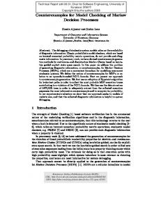
of the system. A famous quotation from 2008 by one of the founders of the concept of model checking, Edmund Clarke, stresses the importance of counterexamples: “It is impossible to overestimate the importance of the counterexample feature. The counterexamples are invaluable in debugging complex systems. Some people use model checking just for this feature. [Cla08]” To give a first intuition, consider a so-called Kripke structure [Kri63] which is a simple model to represent the behavior of a system. Intuitively, the states of the system are modeled by nodes of a graph. Possibilities to move between the states are indicated by transitions. Moreover, every state has a certain set of properties. A toy example can be found below, where from the initial state s1 transitions lead to the states s2 and s3 . Additionally, every state is equipped with a self-loop. The state s2 is labeled with the property

CRITICAL

indicating an undesired behavior.

s2

{CRITICAL}

s1 s3

The specification we want to investigate is that a critical state is never reached; formally we have the LTL formula ¬◊CRITICAL, i. e., “it is not possible to finally reach a state which is labeled

with

CRITICAL ”.

This property is clearly violated by the path leading from s1 to s2 , which also

serves as a counterexample for this property. Classic model checking is based on rigorous exploration of the state space, which leads to serious problems considering the large size of models for real-world scenarios. This is often referred to as the state space explosion problem. Several approaches were developed to overcome this problem. An important one is symbolic model checking which was introduced in 1992 [BCM+ 92] and which is based on a symbolic representation of the state space, e. g., by binary decision diagrams (BDDs) [Bry86]. Dedicated algorithms for these symbolic representations were complemented by SAT-based bounded model checking [CBRZ01], where a SAT solver is used to prove or disprove properties by means of bounded system runs. Another technique is the counterexample-guided abstraction refinement framework (CEGAR) [CGJ+ 00]. Here, verification is performed on abstract systems which—if the abstraction is too coarse—may be refined with the help of counterexamples that are spurious, which means that they do not form a counterexample for the original system. This procedure goes on until a counterexample is found that is not spurious or until the property can be proven to be true. Besides being a guide in debugging a system, counterexamples play an important role in automated verification techniques. As mentioned before, the key ingredient for CEGAR approaches,

2

besides a feasible abstraction, are counterexamples. Another application is in model-based testing [FWA09]. A system is tested via a model, a so-called blueprint of the system. Counterexamples which are obtained during this procedure can be used to correct the original system. Amongst others, these applications, which are of great relevance in practical settings, led to active research on the generation and the representation of counterexamples [GMZ04, CGMZ95, BP12, SB05]. As illustrated by the example above, if a system is simple enough to be modeled sufficiently accurate as a Kripke structure, and if the violated specification is given as a linear-time property, a counterexample is given by a path through the Kripke structure inducing the violation. These counterexamples can be generated on-the-fly during the model checking procedure. For CTL properties, the representation of counterexamples requires a more complex tree-like structure [CJLV02]. For further information, we refer to [CV03]. All the above-mentioned methods were mainly developed for mere digital circuits. The realworld behavior of many processes is inherently stochastic, take for instance randomized algorithms, fault-tolerant systems, or communication networks where certain aspects can only be captured via probabilities. For a network protocol, a useful property would be “The probability of having a message delivered is at least 99.9%.” Referring to a benchmark we use in this thesis, assume a crowd of nodes in a network [RR98], where each member has a probabilistic choice of delivering a message or routing it to another—again randomly determined—node of the network in order to establish anonymity. Assuming “bad” members of the crowd that want to identify the sender of the message, a question would then be “What is the probability that the sender of a message is identified by a bad member?”. Answering such quantitative questions is the comprehensive topic of this thesis. Probabilistic model checking summarizes techniques to analyze systems where transitions are augmented with probabilities. Discrete-time Markov chains (DTMCs) are a popular model to represent probabilistic behavior. Their invention can be traced back to the Russian mathematician Andrey Andreyevich Markov in 1906. For standard textbooks we refer to [KS69, Kul95]. In a nutshell, DTMCs are Kripke structures whose transitions induce a discrete probability distribution over successor states. For DTMCs, properties like “The probability of reaching a critical state is at most 10−5 ” are considered. Markov decision processes (MDPs) and probabilistic automata (PAs) add the feature of a nondeterministic choice of probability distributions to DTMCs. To verify properties, a scheduler is needed to resolve this nondeterminism yielding a DTMC. Such a scheduler then induces a probability measure on this DTMC, for instance the maximal probability for a certain property. We formulate properties like “What is the maximal probability of reaching a critical state”? Standard approaches reduce model checking for DTMCs to solving a linear equation system, while for MDPs an optimization problem is used to compute maximal or minimal probabilities depending on the scheduler, e. g., using linear programming. A detailed description of the basic techniques can be found in [BK08]. For an overview of the state-of-the-art we refer to [Kat13, KNP07]. As for other models, the state space explosion is also a problem for probabilistic systems. Much

3

effort has been put into adapting well-known concepts to this setting. The usage of symbolic data structures via BDDs and multi-terminal binary decision diagrams (MTBDDs) [FMY97] was proposed [BCH+ 97]. For an overview of efficient algorithms and a discussion about hybrid approaches regarding a mixture between symbolic and explicit approaches we refer to [Par02]. For many large or even infinite systems, these methods do still not work. Therefore, one research branch is to develop dedicated abstraction techniques such as probabilistic CEGAR [HWZ08, CV10] or game-based abstraction [KKNP10, Wac10]. The most prominent probabilistic model checker available for the largest variety of models and properties is PRISM [KNP11] developed at the University of Oxford, UK. A very competitive tool is MRMC [KZH+ 11] which has been developed at RWTH Aachen University, Germany. For a comparison, see [JKO+ 07]. Moreover, PRISM offers a large selection of benchmarks [KNP12]; some of them are used throughout this thesis. The generation of counterexamples for probabilistic systems is the main focus of this thesis. Consider the DTMC which is depicted below. With probability 0.05, the successor of the initial state s1 is s2 , and with probability 0.45 the successor is s3 . With probability 0.5, the successor is s1 itself. The states s2 and s3 have self-loops with probability 1 which means that once an execution enters one of those states it will stay there almost surely. For this DTMC, the overall probability to reach the critical state s2 is 0.1. The underlying computations are discussed later. Intuitively, the probability of all paths leading to s2 has to be considered.

0.5

s1

s2

0.05

{CRITICAL} 1

0.45

s3

1

Now consider the quantitative property “The probability of reaching the critical state is less than or equal to 0.05”. This property is violated, as the actual probability is equal to 0.1. Forming a counterexample is not as trivial as for the preceding Kripke structure. The path leading from s1 to s2 has probability 0.05. This path itself does not violate the property. However, the path looping one time on state s1 and then taking the transition to s2 has probability 0.5 · 0.05 = 0.025. The

two paths together have a probability mass of 0.075 which is larger than the allowed probability of 0.05. The set of these two paths serves as a counterexample to the property. The first publications on the generation of counterexamples for DTMCs were [AHL05, AL06, HK07a, DHK08, ADvR08, HKD09, AL10]. The related work is discussed in the corresponding chapter. Let us, however, give a short intuition on the approach that was made in [HK07a, HKD09]: As mentioned before, a counterexample is a set of paths whose joint probability mass exceeds a certain probability threshold. These paths are evidences for a certain property, e. g., for reaching a target state. As only paths describing stochastically independent events are considered;

4

their probabilities can just be added when computing the probability of a whole set of evidences. In [HK07a, HKD09], graph algorithms are utilized to compute a minimal counterexample. In particular, the probabilities are altered such that the most probable paths now correspond to the shortest paths when adding the altered values. Then, a k-shortest path search [Epp98] yields the k most probable paths leading to a target state. As soon as the probability mass of the thereby computed paths is large enough, the search terminates yielding a counterexample that is minimal in terms of the number of paths. Note that the value of k is determined on-the-fly such that the search continues until enough probability mass is accumulated. Consider again the DTMC depicted above and the property “The probability of reaching a critical state is less than 0.1”. The first three paths leading from s1 to s2 in descending order of their probabilities are: π1 = s1 , s2

probability: 0.05

π2 = s1 , s1 , s2

probability: 0.025

π3 = s1 , s1 , s1 , s2

probability: 0.00125

The probability mass of these three paths is 0.07625, which is still too small to induce a counterexample. In fact, to reach the bound of 0.1, all paths leading from s1 to s2 need to be considered, which are infinitely many. The shortest path algorithm as described above would therefore not terminate, while errors might occur as the probabilities of the paths become infinitesimally small. This simple example illustrates one major drawback of counterexamples that are represented as sets of paths: Many paths are similar except for their number of loop-iterations, which calls for a special treatment of loops. Although the generation of counterexamples covers the most important part of this thesis, we have a short excursion to another research direction. Consider systems where no certain probabilities are fixed. At an early design stage, this is a realistic assumption. Determining appropriate probabilities is an own research field called fitting [SR13, TBT06]: In model-based performance analysis, probability distributions are generated from experimental measurements. Therefore, probabilities are handled as parameters yielding parametric discrete-time Markov chains (PDTMCs). Transition probabilities are then interpreted as functions in the system’s parameters. Using these functions, one can, e. g., find appropriate values of the parameters such that certain properties are satisfied, or analyze the sensitivity of reachability probabilities under small changes in the parameters. Standard methods for DTMC model checking such as solving a linear equation system are not feasible for PDTMCs, since the resulting equation system would be non-linear. Consider a modification of the DTMC shown above, where the probability to reach the critical state s2 is now described by a parameter p ∈ [0, 1]. Going from s1 to the uncritical state s3 has probability 9p indicating that the probability of going there should be much

higher than going to s2 , which happens with probability p. The self-loop on s1 is described by q ∈ [0, 1] which again has implicit dependencies to p, if well-defined probability distributions

5

1.1. CONTRIBUTIONS AND STRUCTURE OF THIS THESIS

are considered.

q

s1

s2

p

{CRITICAL} 1

9p

s3

1

Instantiating p with 0.05 yields that the probability of going from s1 to s3 is 0.45 as in the DTMC above. Furthermore, as outgoing probabilities for each state have to sum up to 1 we know that p + 9p + q = 1 yielding q = 0.5. What we already see in this simple example is that there are certain additional constraints for parameter evaluations that need to be taken care of. These complications demand dedicated model checking procedures, the only one publicly available so far being implemented in PARAM [HHWZ10].

1.1 Contributions and structure of this thesis In this section, we describe our approaches that are presented in this thesis and point to the corresponding chapters. Apart from the contributions, we present detailed foundations needed throughout this work in Chapter 2. The related work that has been done before or during the period of this thesis is listed on an intuitive level in Chapter 3. After the theoretical approaches we describe our implementations and tools followed by an experimental evaluation in Chapter 8. The thesis concludes with a short summary and an outlook to future work in Chapter 9.

SCC-based model checking As we have indicated before, benchmarks with a complex loop structure pose a difficult problem for probabilistic counterexample generation. Many paths have to be collected that are similar to each other except for the number of iterations of the same loops. In order to exploit this fact, we developed an abstraction scheme for DTMCs based on the strongly connected components (SCCs) of the underlying directed graph of an input DTMC. First, the SCCs are determined. By heuristically ignoring those states of an SCC to which there is a transition from outside the SCC, it is decomposed into further SCCs. In the context of the original graph we call these SCCs sub-SCCs. This process is iterated until only single states remain. By a subsequent bottom-up computation, the probability of reaching states outside each sub-SCC from its formerly ignored states is computed, while the sub-SCCs are replaced by abstract states. In the end, this gives the probability of reaching the set of target states from the unique initial state. This method was published in [11]. An extension of this work was applied to PDTMCs yielding rational functions that describe reachability probabilities for each sub-SCC. As this induces very large functions even in the early computation steps, they need to be cancelled in each step. This involves the costly computation

6


of the greatest common divisor (GCD) for two polynomials and is therefore not feasible for large benchmarks. However, we were able to partly overcome this problem by developing a new way to compute the GCD on factorizations of the given polynomials. These various methods which were published in [2], improving the computation times in comparison with another approach [HHWZ10] by several orders of magnitude for most of the benchmarks. The approaches are explained in detail in Chapter 4. Summarized, the main contributions are: 1. A novel model checking method for DTMCs that—even in its prototype implementation—is competitive to the well-established tools MRMC [KZH+ 11] and PRISM [KNP11] on many benchmarks having up to one million states. 2. A hierarchical abstraction scheme for DTMCs with respect to their SCC structure. As one of the major benefits, this offers the possibility to search for counterexamples on an abstract graph while each of the abstract states can be refined upon request. 3. A new model checking method for PDTMCs that is faster than the only other available tool,

PARAM [HHWZ10], by orders of magnitude on many common benchmarks. Counterexample generation based on path searching algorithms Based on the SCC abstraction described above, we developed a new method for generating counterexamples on possibly abstract input DTMCs that violate a probabilistic reachability property. We shaped the notion of a critical subsystem of a DTMC which is a sub-graph of the original system where the reachability property is also violated. This highlights the critical parts of the system. Moreover, this subsystem can be seen as a symbolic representation of a set of paths leading from the initial state to one of the target states inside the subsystem; this set forms a counterexample. The search is done in a hierarchical manner by offering the possibility of starting the search on simple abstract graphs and concretizing important parts in order to explore the graph in more detail. The first proposed search algorithm, which we call global search, enumerates paths leading from initial states to target states of the system in descending order of their probabilities, as proposed in [HKD09]. Using these paths, a subsystem is incrementally built until the needed probability mass is reached, i. e., until the subsystem becomes critical. The second search algorithm, called local search or fragment search, incrementally extends a subsystem by finding most probable path fragments that connect paths which were considered before. In comparison to [HKD09], these algorithms lead to improvements by several orders of magnitude in the number of paths that are needed to form counterexamples and for most benchmarks also in terms of computation time. These methods were published in [10]; an extended version is accessible as a technical report [16]. The implementation is publicly available as part of our open-source tool COMICS [6]. The tool offers both a graphical user interface and a command-line version for benchmarking. The GUI depicts the whole hierarchical refinement process which can be completely controlled by the user. Alternatively, many heuristics are offered to automate the process. The only other publicly

7


available tool is DiPro [ALFLS11] which was outperformed on most benchmarks having up to a few million states. These methods for explicit representations of DTMCs are presented in Chapter 5, Sections 5.25.5. The main contributions are: 1. A new hierarchical scheme for finding counterexamples on DTMCs. This allows to search for counterexamples on very large input graphs, as the abstract systems are very small and simply structured. As abstract counterexamples can be concretized, no information is lost, however, not the entire system has to be explored. 2. An improvement in terms of running time, the number of explicitly listed paths, and the possible size of input instances by orders of magnitude using the proposed search algorithms in comparison to previous approaches. 3. The publicly available open-source tool COMICS, which is easy to use and comes with both a command-line version for benchmarking and connecting it with other tools and a GUI where the user can create specialized benchmarks and explore the hierarchical counterexamples in detail. We now report on the adaptions of the aforementioned methods to symbolic data structures. A very successful model checking method is bounded model checking [CBRZ01]. This technique was adapted to counterexample generation for DTMCs in [WBB09] using BDDs and MTBDDs as representations for the input systems. Proceeding from this symbolic representation, modern SAT solvers are used to list the paths that form a counterexample. Thereby, paths leading from the initial state to a target state are encoded by a formula in a way that a satisfying solution of the formula corresponds to such a path. As the bounded model checking approach itself finds arbitrary paths leading from an initial state to one of the target states, the probabilities are ignored. It may therefore be the case that many paths of low probabilities are found while it would lead to an earlier termination to find the paths in descending order of their probabilities. While this informed search is not directly possible for SAT solvers, we tackled this problem by using SAT modulo Theories (SMT) solving instead. This gave us the opportunity to compute a path’s probability not by an external callback but actually to encode the probability computation into the SMT formula and pose restrictions on the minimal probability of a path: A formula is satisfied if and only if the corresponding path has at least a certain probability. This new way of bounded model checking leads to fewer search iterations in most of the cases. These approaches are part of the publications [25, 26] and are not contributions of this thesis. Subsequently, we adapted our previous explicit approaches—namely the counterexample representation as critical subsystems and the fragment search approach—to the setting of bounded model checking. In combination we were able to achieve remarkable improvements to the applicability of bounded model checking for many test cases as reported in [7, 3].

8


In order to prefer more probable paths during the search process, we guide the SAT solver during its variable assignments. Considering partial assignments of variables that encode states of the input system, one can determine which possible paths can be encoded by the remaining, still unassigned, variables. We developed a heuristic which forces the SAT solver to choose assignments that induce more probable path fragments. Even though these bounded model checking approaches improved the previous works, they were in general still not applicable to very large DTMCs. We therefore saw the need to investigate possibilities of working directly on the symbolic representations instead of letting a SAT solver enumerate paths. By that time, the only available fully symbolic method for the generation of counterexamples was an adaption of the approach given in [HKD09] to symbolic data structures [GSS10]. As this approach was only a sort of proof-of-concept to show that one can compute the kshortest paths directly on an MTBDD which was not applicable to large benchmarks, we strived to develop new methods. The first result was presented in [7] and is basically an extension of the search algorithms presented in [10]. Using this method symbolically, we were able to generate

counterexamples for systems with up to 108 states within reasonable time and with low memory consumption. A comprehensive article further improving the methods such that systems with up to 1015 states could be handled, is published in [3]. These symbolic approaches are presented in Chapter 5, Sections 5.6 and 5.7. Altogether the achievements are: 1. An adaption of the usage of critical subsystems and a path-fragment search approach to bounded model checking. 2. A new heuristics to guide a SAT solver to assign states such that more probable paths are preferred. 3. New methods that work directly on the symbolic representation of a DTMC thus enabling the generation of counterexamples for systems consisting of billions of states.

Counterexamples as minimal critical subsystems In [HKD09], the notion of minimal counterexamples in terms of the number of paths was shaped. These might still be very large or even infinite. According to our counterexample representation as critical subsystems, we wanted to explore the possibilities of computing a minimal subgraph of an input DTMC that still violates a certain property. Here, minimality can be defined both in terms of the number of states and in the number of transitions. In any case, the size of the representation is always bounded by the size of the original system. As a first approach we used (non-optimizing) SMT solvers combined with a binary search over the number of involved states to compute such minimal critical subsystems. During the experimental evaluation, it turned out that using mixed integer linear programming (MILP) [Sch86] was more efficient by orders of magnitude than SMT for this setting. Together

9


with a number of optimizations, we were able to solve this minimization problem for many benchmarks with up to roughly ten thousand states. Thereby, we could not only compute very small counterexamples but we could also measure the quality of our previous heuristic approaches as described before. Although larger benchmarks could in general not be solved to optimality within a predefined time limit, all state-of-the-art MILP solvers like SCIP [Ach09], CPLEX [cpl12], or GUROBI [Gur13] are not only able to return the best solution found until the time limit but also to give a lower bound on the value of the optimal solution. This allows to judge the quality of an (possibly not yet optimal) intermediate solution and enables the applicability to larger benchmarks. Moreover, we extended this approach to MDPs, where the problem of finding a minimal critical subsystem has been proven to be NP-hard [CV10]. We published our results for DTMCs and MDPs in [9]. Subsequently, we developed the first directly usable method to compute counterexamples for arbitrary ω-regular properties and DTMCs, which was published in [8]. A comprehensive article containing a method to compute counterexamples for ω-regular properties of MDPs was published in [4]; the correctness and completeness of all MILP and SMT encodings is also included. A corresponding technical report is available [15]. We present these approaches in Chapter 6 where the methods are extended to probabilistic automata (PAs). All in all we developed: 1. A method to compute minimal critical subsystems for reachability properties using SMT and MILP solving. 2. The first method to compute counterexamples for arbitrary ω-regular properties both for DTMCs and PAs.

High-level counterexamples All approaches summarized above use a state-based representation of counterexamples. A very common way to model probabilistic systems like DTMCs, MDPs or PAs is to use an extension [HSM97] of Dijkstra’s guarded command language [Dij75]. Using this language, single modules describing the behavior of system components are specified. These modules can be accumulated to build the entire system, usually a PA, by means of parallel composition. This is the modeling formalism used for PRISM [KNP11], adapted from a stochastic version of Alur and Henzinger’s reactive modules [AH99]. It seems a natural idea to provide counterexamples not at the state space level of the system but at the actual modeling level. On the one hand, this is due to the fact that a system designer likes to be pointed to errors at this level. On the other hand, while the high-level descriptions in the PRISM language are often very compact, they might result in PAs with millions of states where even minimal counterexamples or subsystems are incomprehensible. The idea of such critical model descriptions is to automatically compute fragments of the original description modules that are relevant for the violation of a property. In detail, we determine—

10

1.2. RELEVANT PUBLICATIONS

a preferably small—set of guarded commands that together induce a critical subsystem when composed. As a consequence, in order to correct the system description, at least one of the returned guarded commands has to be changed. Our methodology is as follows: First, the composition of the modules induces a full PA model at the state space level. During the composition, each resulting transition is labeled with unique identifiers of its constituting guarded command(s), i. e., the commands that actually induce this transition. Then, model checking is applied to determine whether a property is violated. The problem of computing a minimal critical command set is then reduced to computing a minimal critical labeling of the PA. Utilizing this flexible problem formulation, we present several alternatives of human-readable counterexamples. Furthermore, we show that this problem is NP-hard, which justifies the usage of an MILP solver. Besides the theoretical principles of our technique, we illustrate its practical feasibility by showing the results of applying a prototypical implementation to various examples from the PRISM benchmark suite. This approach was first presented in [5]. An extended version was published in [1]. This version is also accessible as a technical report [13]. Finally, the high-level approach is explained in Chapter 7. The contributions are: 1. A new approach to constructing counterexamples based on the high-level modeling language for probabilistic systems. 2. A flexible formulation in terms of a minimal critical labeling, enabling the possibility to create human-readable counterexamples.

1.2 Relevant publications In this section we list the articles that contain contributions presented in this thesis. We distinguish peer-reviewed publications such as conference proceedings or journals and technical reports. Afterwards, we give a short note on how the author has contributed to the contents. The section concludes with publications of the author that are not content of this thesis.

1.2.1 Peer-reviewed publications [1] Ralf Wimmer, Nils Jansen, Erika Abraham, and Joost-Pieter Katoen. High-level counterexamples for probabilistic automata. Logical Methods in Computer Science, 11(1:15), 2015. [2] Nils Jansen, Florian Corzilius, Matthias Volk, Ralf Wimmer, Erika Ábrahám, Joost-Pieter Katoen, and Bernd Becker. Accelerating parametric probabilistic verification. In Proc. of QEST, volume 8657 of LNCS, pages 404–420. Springer, 2014.

11


[3] Nils Jansen, Ralf Wimmer, Erika Ábrahám, Barna Zajzon, Joost-Pieter Katoen, Bernd Becker, and Johann Schuster. Symbolic counterexample generation for large discrete-time Markov chains. Science of Computer Programming, 91(A):90–114, 2014. [4] Ralf Wimmer, Nils Jansen, Erika Ábrahám, Joost-Pieter Katoen, and Bernd Becker. Minimal counterexamples for linear-time probabilistic verification. Theoretical Computer Science, 549:61–100, 2014. [5] Ralf Wimmer, Nils Jansen, Andreas Vorpahl, Erika Abraham, Joost-Pieter Katoen, and Bernd Becker. High-level counterexamples for probabilistic automata. In Proc. of QEST, volume 8054 of LNCS, pages 18–33. Springer, 2013. [6] Nils Jansen, Erika Ábrahám, Matthias Volk, Ralf Wimmer, Joost-Pieter Katoen, and Bernd Becker. The COMICS tool – Computing minimal counterexamples for DTMCs. In Proc. of ATVA, volume 7561 of LNCS, pages 349–353. Springer, 2012. [7] Nils Jansen, Erika Ábrahám, Barna Zajzon, Ralf Wimmer, Johann Schuster, Joost-Pieter Katoen, and Bernd Becker. Symbolic counterexample generation for discrete-time Markov chains. In Proc. of FACS, volume 7684 of LNCS, pages 134–151. Springer, 2012. [8] Ralf Wimmer, Nils Jansen, Erika Ábrahám, Joost-Pieter Katoen, and Bernd Becker. Minimal critical subsystems as counterexamples for ω-regular DTMC properties. In Proc. of MBMV, pages 169–180. Verlag Dr. Kovaˇc, 2012. [9] Ralf Wimmer, Nils Jansen, Erika Ábrahám, Joost-Pieter Katoen, and Bernd Becker. Minimal critical subsystems for discrete-time Markov models. In Proc. of TACAS, volume 7214 of LNCS, pages 299–314. Springer, 2012. [10] Nils Jansen, Erika Ábrahám, Jens Katelaan, Ralf Wimmer, Joost-Pieter Katoen, and Bernd Becker. Hierarchical counterexamples for discrete-time Markov chains. In Proc. of ATVA, volume 6996 of LNCS, pages 443–452. Springer, 2011. [11] Erika Ábrahám, Nils Jansen, Ralf Wimmer, Joost-Pieter Katoen, and Bernd Becker. DTMC model checking by SCC reduction. In Proc. of QEST, pages 37–46. IEEE Computer Society, 2010.

1.2.2 Technical reports [12] Nils Jansen, Florian Corzilius, Matthias Volk, Ralf Wimmer, Erika Ábrahám, Joost-Pieter Katoen, and Bernd Becker. Accelerating parametric probabilistic verification. CoRR, 2013. [13] Ralf Wimmer, Nils Jansen, Andreas Vorpahl, Erika Ábrahám, Joost-Pieter Katoen, and Bernd Becker. High-level counterexamples for probabilistic automata. Technical report, University of Freiburg, 2013.

12


[14] Nils Jansen, Erika Ábrahám, Maik Scheffler, Matthias Volk, Andreas Vorpahl, Ralf Wimmer, Joost-Pieter Katoen, and Bernd Becker. The COMICS tool - Computing minimal counterexamples for discrete-time Markov chains. CoRR, 2012. [15] Ralf Wimmer, Nils Jansen, Erika Ábrahám, Joost-Pieter Katoen, and Bernd Becker. Minimal counterexamples for refuting ω-regular properties of Markov decision processes. Reports of SFB/TR 14 AVACS, 2012. [16] Nils Jansen, Erika Ábrahám, Jens Katelaan, Ralf Wimmer, Joost-Pieter Katoen, and Bernd Becker. Hierarchical counterexamples for discrete-time Markov chains. Technical report, RWTH Aachen University, 2011.

1.2.3 A note on contributions by the author All publications listed above were the result of the work of many people, as can be seen by the numerous authors. Most of the results were jointly achieved in many discussions via phoning, texting and of course many meetings in Aachen, Freiburg, Dagstuhl, or at conferences. However, for this thesis it is necessary to somehow measure my contributions. I will therefore now chronologically, i. e., according to the publication date, explain what I explicitly contributed. In general, I co-wrote all publications and technical reports. I will therefore only talk about the development of the results. To begin with, in [11] the basic idea was developed by me together with Erika Ábrahám in various initial discussions while getting familiar with the topic of probabilistic systems. The implementation was mainly done by me. The results of [10, 16] again were developed together by Erika Ábrahám and me, while the implementation was done by a student under my supervision. The tool presented in [6, 14] was developed by me with great help of a number of students which are mentioned in the acknowledgements. Extending the former approaches on counterexample generation to symbolic data structures was inspired by a previous work of Ralf Wimmer and initiated by me, which led to [7]. The implementation was done by a student and me. I was the main developer of the further improvements which led to the extensions in [3]. The initial idea of [9] came up at a discussion in Dagstuhl and was initially carried out by Ralf Wimmer. I developed several improvements to get scalable methods and worked with Ralf Wimmer and Erika Ábrahám on most of the proofs. The key idea for some of the extensions in [4, 15] was given by Joost-Pieter Katoen while Ralf Wimmer and I initiated the further development. Most of the details were worked out in several discussions in Aachen and Dagstuhl. The implementations for [4, 15] were done by Ralf Wimmer and me together with a student. Ralf Wimmer had the idea for [5, 13] while he and I together worked on all the details and again did the implementation together with a student.

13

1.3. FURTHER PUBLICATIONS

The part of the results of [2, 12] that is presented in this thesis were mainly developed by me while the implementation was done by a student under the supervision of Florian Corzilius and me.

1.3 Further publications Additionally, we list the publications of the author that are not contained in this thesis. [17] Christian Dehnert, Sebastian Junges, Nils Jansen, Florian Corzilius, Matthias Volk, Harold Bruintjes, Joost-Pieter Katoen, and Erika Abraham. Prophesy: A probabilistic parameter synthesis tool. In Proc. of CAV, 2015. To appear. [18] Friedrich Gretz, Nils Jansen, Benjamin Lucien Kaminski, Joost-Pieter Katoen, Annabelle McIver, and Federico Olmedo. Conditioning in probabilistic programming. In Proc. of MFPS, LNCS. Springer, 2015. To appear. [19] Shashank Pathak, Erika Ábrahám, Nils Jansen, Armando Tacchella, and Joost-Pieter Katoen. A greedy approach for the efficient repair of stochastic models. In Proc. of NFM, volume 9058 of LNCS, pages 295–309. Springer, 2015. [20] Tim Quatmann, Nils Jansen, Christian Dehnert, Ralf Wimmer, Erika Abraham, Joost-Pieter Katoen, and Bernd Becker. Counterexamples for expected rewards. In Proc. of FM, volume 9109 of LNCS, pages 435–452. Springer, 2015. [21] Erika Ábrahám, Bernd Becker, Christian Dehnert, Nils Jansen, Joost-Pieter Katoen, and Ralf Wimmer. Counterexample generation for discrete-time Markov models: An introductory survey. In Proc. of SFM, volume 8483 of LNCS, pages 65–121. Springer, 2014. [22] Christian Dehnert, Nils Jansen, Ralf Wimmer, Erika Ábrahám, and Joost-Pieter Katoen. Fast debugging of PRISM models. In Proc. of ATVA, volume 8837 of LNCS, pages 146–162. Springer, 2014. [23] Daniel Neider and Nils Jansen. Regular model checking using solver technologies and automata learning. In Proc. of NFM, volume 7871 of LNCS, pages 16–31. Springer, 2013. [24] Erika Ábrahám, Nadine Bergner, Philipp Brauner, Florian Corzilius, Nils Jansen, Thiemo Leonhardt, Ulrich Loup, Johanna Nellen, and Ulrik Schroeder. On collaboratively conveying computer science to pupils. In Proc. of KOLI, pages 132–137. ACM, 2011. [25] Bettina Braitling, Ralf Wimmer, Bernd Becker, Nils Jansen, and Erika Ábrahám. Counterexample generation for Markov chains using SMT-based bounded model checking. In Proc. of FMOODS/FORTE, volume 6722 of LNCS, pages 75–89. Springer, 2011.

14

1.4. HOW TO READ THIS THESIS

[26] Bettina Braitling, Ralf Wimmer, Bernd Becker, Nils Jansen, and Erika Ábrahám. SMTbased counterexample generation for Markov chains. In Proc. of MBMV, pages 19–28. Offis Oldenburg, 2011. [27] Erika Ábrahám, Philipp Brauner, Nils Jansen, Thiemo Leonhardt, Ulrich Loup, and Ulrik Schroeder. Podcastproduktion als kollaborativer Zugang zur theoretischen Informatik. In Proc. of DeLFI, volume 169 of LNI, pages 239–251. Gesellschaft für Informatik, 2010.

1.4 How to read this thesis In order to ease the reading of this work, we begin every chapter with a short paragraph containing a Summary of what is presented in this chapter. This is followed by a paragraph called Background, which contains the preliminaries that are relevant for this chapter together with a link to the according definitions or sections in the chapter about Foundations.

1.4.1 Algorithms All algorithms are given in pseudo code and more or less mathematically formal, depending on the problem at hand. For every algorithm we list all used parameters, variables and methods afterwards. This is followed by an explanation on how the algorithm proceeds. A small toy example can be seen below: Algorithm 1 Integer ExampleAlgo(Integer x) begin Integer y := 0 y := x return testMethod( y ) end

(1) (2) (3)

Parameters y is an integer parameter.

Return value The result of testMethod(y) is returned.

Variables x is an integer variable. If variables are not initialized, they are considered to have the value ;.

15

1.4. HOW TO READ THIS THESIS

Methods testMethod does something with integer parameter y and returns an integer value.

Procedure The algorithm proceeds as follows: First, the variable y is initialized to 0. Then, it is set to the value of the parameter x. Finally, the result of testMethod called with parameter y is returned.

1.4.2 Problem encodings In some parts of this thesis, problems are handled by utilizing solving techniques. Therefore, we have to encode a solution to a problem by means of constraints that have to be satisfied. As these constraints are not very intuitive at some parts, we present all encodings in the following form.

Intuition Here we give the intuition of the problem that is to be encoded. In our toy example we want to ensure that all used variables sum up to a value that is less than or equal to 1.

Variables x ∈ [0, 1] ⊆ R is a real-valued variable between 0 and 1 y ∈ {0, 1} is an integer variable that can take the values 0 or 1

Constraints x+ y ≤1

(1.1)

Explanation The sum of x and y is forced to take a value less than or equal to 1 by Constraint 1.1. This implies that if the integer variable y is assigned 1, x has to be assigned 0. If y is assigned 0, x can be assigned any possible value out of R between 0 and 1.

Formula size The formula size is constant.

16

CHAPTER

2

Foundations

In this chapter we lay the foundations needed for the results presented in this thesis. After shortly fixing some basic notations we formalize the probabilistic models that are subject of our methods. We present the different specification languages as well as corresponding verification techniques for the introduced models. We also discuss the concept of symbolic representations of state spaces, which is used for large systems. We introduce some basic solving techniques which are used throughout the thesis as blackbox algorithms. The chapter concludes with an introduction to probabilistic counterexamples.

2.1 Basic notations and definitions Numbers, intervals and matrices We denote the set of real numbers by R, the rational numbers by Q, the natural numbers including 0 by N, and the integer numbers by Z. By R>0 we denote the positive real numbers and by R≥0 the nonnegative real numbers. The same holds for Q>0 , Q≥0 , N>0 , Z>0 , and Z≥0 , respectively.

Let [0, 1] ⊆ R denote the closed interval of all real numbers between 0 and 1, including the

bounds; (0, 1] ⊆ R denotes the open interval of all real numbers between 0 and 1 excluding 0.

A ∈ Rm×n denotes a matrix A with m rows and n columns with values out of R. The same

holds for Nm×n , Qm×n and Zm×n , respectively.

Sets Let X , Y denote arbitrary sets. If X ∩ Y = ; holds, we write X ] Y for the disjoint union of

the sets X and Y . As usual, we write X ⊆ Y if X is subset of Y . If additionally Y \ X 6= ; holds,

we write X ⊂ Y .

By 2X = {X 0 | X 0 ⊆ X } we denote the power set of X . By (X i )i≥0 we denote an arbitrary family

2.1. BASIC NOTATIONS AND DEFINITIONS of sets X i . We call a set P ⊆ 2X \ ; a partition of X if [

P0 = X

∀P 0 , P 00 ∈ P : P 0 6= P 00 ⇒ P 0 ∩ P 00 = ;

and

P 0 ∈P

holds. The elements of the partition P are called blocks. By X ω we denote the set of all infinite sequences of elements from X : x 1 , x 2 , . . . for x i ∈ X , i > 0. X n denotes the set of all finite sequences x 1 , . . . , x n of X for x i ∈ X , 1 ≤ i ≤ n.

Distributions Let X be a finite or countably infinite set. A probability distribution over X P is a function µ: X → [0, 1] ⊆ R1 with x∈X µ(x) = µ(X ) = 1. A sub-stochastic distribution P over X is a function µ: X → [0, 1] ⊆ R such that x∈X µ(x) = µ(X ) ≤ 1. We denote the

set of all (sub-stochastic) distributions on X by Distr(X ) or subDistr(X ), respectively. The set supp(µ) = {x ∈ X | µ(x) > 0} is called the support of µ for a (sub-stochastic) distribution µ. We

write µ0 ⊆ µ for µ, µ0 ∈ subDistr(X ), if for all x ∈ X it holds that µ0 (x) > 0 implies µ0 (x) = µ(x) and µ0 (x) = 0 for µ(x) = 0. If for µ ∈ Distr(X ) it holds that µ(x) = 1 for one x ∈ X and µ( y) = 0 for all y ∈ X \ {x}, µ is called a Dirac distribution.

Polynomials For an arbitrary function f : X → Y we denote the domain of f by dom( f ) = X .

Let V denote a set of variables. The domain of a variable x ∈ V is denoted by dom(x). The S domain of the whole set of variables is denoted by dom(V ) = x∈V dom(x). Definition 1 (Polynomial, monomial) Let V = {x 1 , . . . , x n } be a set of variables with

dom(V ) = R. A monomial m over V is the product of a coefficient a ∈ Z and variables from V :

e

m := a · x 11 · . . . · x nen with ei ∈ N for all 1 ≤ i ≤ n. The set of all monomials over V is denoted by MonV . A polynomial g over V is a sum of monomials over V :

g := m1 + . . . + ml with mi ∈ MonV , 1 ≤ i ≤ l. The set of all polynomials over V is denoted by PolV .

We also need the notion of a rational function, which is the fraction

g1 g2

of two polynomials.

Thereby, this function is clearly not defined at the roots of the denominator. We additionally restrict the denominator to be unequal to 0. By g2 6= 0 we state that the polynomial g2 cannot be simplified to 0 which is necessary to define the division by g2 . Moreover, the rational function g1 g2

is not defined at the roots of g2 . In order to have valid evaluations of a rational function for

our algorithms, we later restrict these evaluations accordingly. 1

For the algorithms in this thesis, probabilities are from Q.

18

2.2. PROBABILISTIC MODELS

Definition 2 (Rational function) Let V = {x 1 , . . . , x n } be a set of variables with dom(V ) = R. A rational function f over V is given by f := all rational functions over V is denoted by RatV .

g1 g2

with g1 , g2 ∈ PolV and g2 = 6 0. The set of

2.2 Probabilistic models We introduce the different probabilistic models which are used throughout this thesis. All our models are based on discrete time, i. e., instantaneous transitions discretely model the advance of time by one time unit. Possible interpretations are that scenarios like the ticks of clock are modeled or that for the probabilistic information the amount of time that is used is irrelevant. Continuous time models like continuous time Markov chains are out of the scope of this thesis. For an overview of different models, both discrete-time and continuous-time, we refer to [Fel68, How79].

2.2.1 Discrete-time Markov chains Intuitively, Markov Chains are transition systems where at each state there is a probabilistic choice for the successor state. If the time model is discretized such that we have instantaneous transitions, we speak of discrete-time Markov chains. The probability of going from a state to another one depends only the current state, i. e., this probability is history independent of the path taken so far. This property is called the Markov property. This is due to the fact, that a DTMC is actually a stochastic process whose random variables are all geometrically distributed. For details we refer to [BK08, Chapter 10]. Let in the following AP be a finite set of atomic propositions. Definition 3 (DTMC) A discrete-time Markov chain (DTMC) is a tuple D = (S, I, P, L) with: • S a countable set of states • I ∈ subDistr(S) an initial distribution • P : S → subDistr(S) a transition probability matrix • L : S → 2AP a labeling function.

Remark 1 (Finite state space) Note that although the set of states is allowed to be countably infinite, for our algorithms we assume finite state spaces. The probability of going to a state s0 ∈ S from a state s ∈ S in one step is given by the

corresponding entry P(s, s0 ) in the transition probability matrix. The probability to reach a set P S 0 ⊆ S of states from s in one step is given by P(s, S 0 ) = s0 ∈S 0 P(s, s0 ). Analogously, P(S 0 , s) = 19


0.5

s2

s4 0.7

0.25

0.5

0.5

0.5

s0

0.3 0.5

s1

s3

0.25

{target} 1

0.5 1

s5

0.25

s8

s6 0.25

0.5

0.5

1

s7 Figure 2.1: Example DTMC D

P

s0 ∈S 0

P(s0 , s) holds. The initial distribution determines the probability of starting at certain

states. We denote the set of states where this probability is not 0, the initial states, by InitD = {s ∈ S | I(s) > 0} .

Example 1 Consider a DTMC D = (S, I, P, L) with S = {s0 , . . . , s8 }, I(s0 ) = 1, L(s3 ) = {target} and L(s) = ; for all s 6= s3 . The transition probability matrix is given by: 

0 0.5 0.25

 0 0  0 0.5   0 0  P = 0 0.7  0 0  0 0  0 0  0

0

0.5 0 0 0 0 0 0 0

0

0

0.25

0

0

0.5

0

0

0

0

0



 0   0 0.5 0 0 0 0    1 0 0 0 0 0   0.3 0 0 0 0 0    0 0 0 1 0 0   0.5 0 0 0 0.5 0   0 0 0.25 0.25 0 0.5  0 0 0 0 0 1

The DTMC D is depicted in Figure 2.1. Every state has (possibly empty) sets of predecessors and successors:

20


Definition 4 (Predecessors, successors) For a DTMC D = (S, I, P, L), the successors of a state s ∈ S are given by

succD (s) = {s0 ∈ S | P(s, s0 ) > 0} . The predecessors of s ∈ S are given by predD (s) = {s0 ∈ S | P(s0 , s) > 0} . A state s ∈ S with succD (s) = {s} is called an absorbing state. Remark 2 (Sub-stochastic distribution) Our definition of a DTMC allows sub-stochastic distributions for the initial distribution I and for the transition probability matrix P. Usually, the sum of probabilities is required to be exactly 1. This can be obtained by defining for a DTMC D a new DTMC D 0 = (S 0 , I 0 , P 0 , L 0 ) where all “missing” probabilities are directed to a new sink state s⊥ : • S 0 = S ] {s⊥ }  • I 0 (s) =

 I(s) if s ∈ S 0 otherwise 

0

P(s, s )     1 • P 0 (s, s0 ) = P   1 − s0 ∈S P(s, s0 )    0

if s, s0 ∈ S

if s = s0 = s⊥

if s ∈ S, s0 = s⊥ if s = s⊥ , s0 ∈ S

 • L 0 (s) =

 L(s) if s ∈ S ; if s = s⊥ .

We often directly or indirectly refer to the graph which is induced by a DTMC D: Definition 5 (Graph of a DTMC) For a DTMC D = (S, I, P, L), the underlying directed graph of D is given by GD = (S, ED ) with the set of edges

ED = {(s, s0 ) ∈ S × S | s0 ∈ succD (s)}.

We call the edges of GD also transitions. A transition (s, s0 ) ∈ ED has a source state s and a

destination state s0 . We denote the number of states by |S| = nD and the number of transitions by |ED | = mD .

21


Remark 3 (Explicit graph representation) If the matrix is explicitly stored in data-structures like vectors or 2-dimensional matrices, we speak of an explicit graph representation. This representation is used, for instance, by the probabilistic model checker MRMC [KZH+ 11]. This is the counterpart of symbolic graph representations which are discussed in Section 2.4.

Sparse matrix representation As indicated by the previous example, typically the transition probability matrices of DTMCs contain many entries having the value 0, i. e., the matrices are very sparse. For many operations it is beneficial to use so-called sparse matrix representations. Three vectors row, col and val are used to store A. The vector val stores all non-zero entries in a certain order. Vector col stores the indices of the columns of the values in val. row stores pointers to the other vectors such that the ith element of row points to the first entry of row i in the original matrix A represented by col and val. This compact representation is beneficial for numerical operations like matrix-vector multiplications. For more details, we refer to [Par02, Ste94]. If only a part of the states of a DTMC is to be considered, we use the notion of a subsystem.

Definition 6 (Subsystem of a DTMC) For a DTMC D = (S, I, P, L), a subsystem of D is a DTMC D 0 = (S 0 , I 0 , P 0 , L 0 ) with: • S0 ⊆ S • I 0 (s) = I(s) for all s ∈ S 0 • P 0 (s, s0 ) = P(s, s0 ) for all s, s0 ∈ S 0 • L 0 (s) = L(s) for all s ∈ S 0 . We write D 0 v D.

Paths of DTMCs Assume in the following a DTMC D = (S, I, P, L). We fix some notations regarding the paths that go through a DTMC.

Definition 7 (Path of an DTMC) A path π of a DTMC D = (S, I, P, L) is a finite or infinite sequence π = s0 , s1 , . . . of states such that si ∈ S and P(si , si+1 ) > 0 for all i ≥ 0.

If π is a finite path π = s0 , s1 , . . . , sn we define the length of π by |π| = n. The length of an infinite path π is |π| = ∞. The first state π of a path is denoted by first(π) = s0 ; the last state of a finite

path π is denoted by last(π) = sn . By πi we denote the prefix of π of length i. Let π(i) denote the ith state of π. By s0 , . . . , s j , (s j+1 , . . . , sk )∗ , . . . for 0 ≤ j < k ≤ |π| and s j = sk we denote a set of paths that are equal except for the number of iterations of the loop s j , . . . , sk .

22


Example 2 (Loops) Consider the DTMC D from Example 1. The path π1 = s0 , s1 , s2 , s1 , s3 contains

a loop πl = s1 , s2 , s1 . The set of all paths differing only in the number of iterations of this loop is denoted by Π = s0 , s1 , (s2 , s1 )∗ , s3 . For instance, π2 = s0 , s1 , s2 , s1 , s2 , s1 , s3 ∈ Π. Moreover, the path π3 = s0 , s1 , s3 not traversing that loop is also part of Π.

By PathsD we denote the set of all paths of D and by PathsD (s) the set of all paths of D that start

D in state s ∈ S. Analogously, we define the sets of finite paths PathsD fin and infinite paths Pathsinf as

D D 0 0 well as PathsD fin (s) and Pathsinf (s), respectively. For states s and s we denote by Pathsfin (s, s ) the

set of finite paths that start in s0 and end in s00 . For sets of states S 0 ⊆ S and S 00 ⊆ S we denote

0 00 by PathsD finite paths that start in a state s ∈ S 0 and end in a state s00 ∈ S 00 , fin (S , S ) the set of S S D 0 00 0 00 formally PathsD s0 ∈S 0 s00 ∈S 00 Pathsfin (s , s ). Sometimes we omit the subscript D if it fin (S , S ) =

is clear from the context.

D The concatenation of a finite path π1 ∈ PathsD fin and a finite or infinite path π2 ∈ Paths with

last(π1 ) = first(π2 ) is denoted by π = π1 π2 = π1 (0), . . . , π1 (|π1 − 1|), π2 (0), π2 (1), . . . The set

of all prefixes of π ∈ PathsD is pref D (π) = {πi | 0 ≤ i ≤ |π|}. If |π1 | < |π| and π1 ∈ pref D (π) hold, π1 is called a real prefix of π.

We call a set R of paths prefix-free, if for all π1 , π2 ∈ R ⊆ PathsD it holds that either π1 = π2 or

D π1 ∈ / pref D (π2 ). By PathsD k ⊆ Pathsfin we denote all finite paths of length k ∈ N.

Definition 8 (Trace) The trace of a finite or infinite path π = s0 , s1 , . . . of a DTMC D =

(S, I, P, L) is given by the sequence trace(π) = L(s0 ), L(s1 ) . . .

We sometimes use state names as atomic propositions, i. e., s ∈ L(s) for s ∈ S.

Probability measure on DTMCs In order to define a probability measure for sets of infinite paths, we first have to recall the general notions of σ-algebras and associated probability measures, which together form a probability space. Definition 9 (σ-algebra) Let X be a set. A set Σ ⊆ 2X is called a σ-algebra over X if: 1. X ∈ Σ (underlying set contained) 2. Y ∈ Σ ⇒ (X \ Y ) ∈ Σ (closed under complement) 3. Y1 , Y2 , . . . ∈ Σ ⇒ (

S i≥1

Yi ) ∈ Σ (closed under countable union).

From Conditions 1 and 2 it follows that ; ∈ Σ. In order to assign probabilities to the elements

of a σ-algebra, a probability measure is associated.

Definition 10 (Probability measure) Let Σ be a σ-algebra over a set X . A function µ: Σ →

[0, 1] ⊆ R is called a probability measure if: • µ(;) = 0 (empty set is assigned zero)

23

2.2. PROBABILISTIC MODELS • ∀Y ∈ Σ: µ(Y ) = 1 − µ(X \ Y ) (closed under complement) • For all families (Yi )i≥1 of pairwise disjoint sets Yi ∈ Σ it holds that µ(

[ i≥1

Yi ) =

X i≥1

µ(Yi ) (countable additivity).

These elements form a probability space. Definition 11 (Probability space) Let Σ be a σ-algebra over a set X and µ: Σ → [0, 1] ⊆ R an associated probability measure. The triple (X , Σ, µ) is called a probability space.

In the literature, X is often referred to as the sample space and the elements of the σ-algebra are called events. For more details we refer to standard books about measure theory, such as [BW07, BT02]. We now associate a probability space to a DTMC D. The set Pathsinf of infinite paths of D

forms the sample space. In order to define a suitable σ-algebra over Pathsinf we define so-called cylinder sets of finite paths. Definition 12 (Cylinder set) The cylinder set of a finite path π = s0 , s1 , . . . , sn ∈ PathsD fin (s0 ) 0 is the set cyl(π) = {π0 ∈ PathsD inf (s0 ) | π ∈ pref D (π )} of all infinite extensions of π.

For a DTMC D and a state s ∈ S, a probability space (Ω, F , PrD s ) can be defined as follows: The Ω sample space Ω = PathsD inf (s) is the set of all infinite paths starting in s. The events F ⊆ 2 are

given by the smallest σ-algebra that contains the cylinder sets of all finite paths in PathsD fin (s), i. e., it is the closure of the cylinder sets under complement and countable union containing Ω. For details we refer to [BK08, Definition 10.10]. The probability of a finite path π = s0 , s1 , . . . , sn is given by the product of all transition probabilities: PD (π) =

n−1 Y i=0

P(si , si+1 )

For paths π of length |π| = 1 we set PD (π) = 1. Two finite paths present two stochastically independent events, if no path is a prefix of the other one, i. e., their cylinder sets are disjoint. If we are interested in the probability of finite paths that start in a specific state, we have  PD s (π) =

PD (π) 0

24

if s0 = s otherwise


The probability measure is extended to sets of paths: For a prefix-free set of finite paths R ⊆ PathsD fin we have

PD (R) =

X

PD (π).

π∈R D For the concatenation of two paths π = π1 π2 ∈ PathsD fin with π1 , π2 ∈ Pathsfin and first(π2 ) =

last(π1 ) = s it holds that PD (π1 ) · PD (π2 ) = PD (π).

The probability of cylinder sets is defined using the measure for finite paths: D PrD s cyl(s0 , s1 , . . . , sn ) = P (s0 , s1 , . . . , sn ) 0

This measure can uniquely be extended to the whole σ-algebra associated with D, yielding the probability measure PrD s : F → [0, 1] ⊆ R [Nor97]. A set Π of paths is called measurable iff 0

Π ∈ F.

Remark 4 (Measure for finite paths) In the following we sometimes let finite paths denote their cylinder sets. Remark 5 (Initial distribution vs. initial state) Instead of defining an initial distribution I for a DTMC D, we often use a single initial state sI . This is no restriction, as every DTMC having an arbitrary initial distribution can be transformed to one having one unique initial state. This

transformation does not affect the satisfaction of the properties we investigate. Let D = (S, I, P, L) be a DTMC. We define D 0 = (S 0 , I 0 , P 0 , L 0 ) with a fresh unique initial state sI ∈ / S: • S 0 = S ] {sI }  • I 0 (s) =

1 0

if s = sI if s ∈ S



I(s0 ) if s = sI , s0 ∈ S   • P 0 (s, s0 ) = P(s, s0 ) if s, s0 ∈ S   0 otherwise  • L 0 (s) =

; if s = sI  L(s) if s ∈ S .

We also write D 0 = (S 0 , sI , P 0 , L 0 ).

Sets of states Throughout this thesis, we often have to argue about certain sets of states. For a DTMC D = (S, I, P, L) and a subset of states K ⊆ S we define the set of input states of K in D

by InpD (K) = {s ∈ K | I(s) > 0 ∨ ∃s0 ∈ S \ K. P(s0 , s) > 0}, i. e., the states inside K that have an 25


incoming transition from outside K. Analogously, we define the set of output states of K in D

by OutD (K) = {s ∈ S \ K | ∃s0 ∈ K. P(s0 , s) > 0}, i. e., the states outside K that have an incoming transition from a state inside K. The set of inner states of K in D is given by K \ InpD (K). We

sometimes omit the subscript D if it is clear from the context. A set of states K in D is called

absorbing in D if the probability to reach a state of OutD (K) is less than 1, i. e., if OutD (K) is not reached with probability 1.

Special sets of states are strongly connected components. Definition 13 (Strongly connected component) Let D = (S, I, P, L) be a DTMC and S 0 ⊆ S

a subset of states with S 0 = 6 ;. S 0 is called a strongly connected sub-component (SCS) of D, if 0 0 for all s, s0 ∈ S 0 there is a path s0 , s1 , . . . , sn ∈ PathsD fin (s, s ) with si ∈ S for all i = 0, . . . , n.

A strongly connected subgraph of D is a called a strongly connected component (SCC) if it

is maximal, i. e., for all strongly connected subgraphs S 00 ⊆ S we have that S 0 6⊂ S 00 . P S 0 is a bottom SCC (BSCC) if it is an SCC and for all s ∈ S 0 we have that s0 ∈S 0 P(s, s0 ) = 1.

Intuitively, from every state of an SCS S 0 every other state in S 0 is reachable inside S 0 . The SCC structure of a directed graph can be determined by Tarjan’s algorithm in linear time [Tar72]. As the set of output states of a BSCC is empty, the probability to visit each state in a BSCC infinitely often is 1. Moreover, if we assume only stochastic distributions, the probability to finally reach a set of absorbing states, i. e., the set of all BSCCs of a DTMC, is 1. This implies that the probability to finally leave a non absorbing SCC is also 1. For details about these properties, we refer to [BK08, Chapter 10.1.2].

2.2.2 Probabilistic automata and Markov decision processes In order to allow both probabilistic and nondeterministic behavior, probabilistic automata and Markov decision processes extend DTMCs by nondeterministic choices for probability distributions over successor states. Definition 14 (PA) A probabilistic automaton (PA) is a tuple M = (S, I, Act, P , L) with: • S a countable set of states • I ∈ subDistr(S) an initial distribution • Act a finite set of actions • P : S → 2Act×subDistr(S) a probabilistic transition relation where P (s) is finite for all s∈S

• L : S → 2AP a labeling function.

If every action α ∈ Act occurs only once at each state of M , the model is called a Markov decision process.

26


Definition 15 (MDP) A discrete-time Markov decision process (MDP) is a probabilistic automaton M = (S, I, Act, P , L) where it holds for all s ∈ S and all α ∈ Act that |{µ ∈ subDistr(S) | (α, µ) ∈ P (s)}| ≤ 1 .

For MDPs, the probabilistic transition relation can also be written as a three-dimensional transition probability matrix of the form P : S × Act → subDistr(S). If possible, we often use this notation.

Remark 6 (Finite state space) As for DTMCs, we assume PAs and MDPs to have a finite state space, see Remark 1. We define sets of predecessors and successors for a state, for a pair of state and action, and for a state and a pair of action and distribution. Definition 16 For a PA M = (S, I, Act, P , L), the predecessors of s ∈ S for α ∈ Act and µ ∈ subDistr(S) are given by:

predM (s, α, µ) = {s0 ∈ S | (α, µ) ∈ P (s0 ) ∧ s ∈ supp(µ)}

predM (s, α) = {s0 ∈ S | ∃µ ∈ subDistr(S). s0 ∈ pred(s, α, µ)} [ predM (s) = predM (s, α). α∈Act

The successors of s ∈ S for α ∈ Act and µ ∈ subDistr(S) are given by: succM (s, α, µ) = {s0 ∈ S | (α, µ) ∈ P (s) ∧ s0 ∈ supp(µ)}

succM (s, α) = {s0 ∈ S | ∃µ ∈ subDistr(S). s0 ∈ succ(s, α, µ)} [ succM (s) = succM (s, α). α∈Act

We sometimes abbreviate pairs of action and distribution by (α, µ) = η ∈ P (s) for a state s ∈ S.

In the following, we overload some notations we originally defined for (sub-)distributions such

that they are also used for pairs of an action α ∈ Act and a (sub-)distribution µ ∈ subDistr(s). For instance, the support of a distribution µ is also defined if a specific action is given: supp(η) = supp(µ) for η ∈ Act × {µ}. We also call (s, η, s0 ) ∈ S × P (s) × S a branch of s.

For a state s ∈ S, a successor state is determined as follows: First, η ∈ P (s) is chosen nonde-

terministically. Then, s0 ∈ supp(η) is determined probabilistically according to the distribution in

η. This yields the transitions (s, η, s0 ) to be taken from s. This process can be repeated infinitely often starting with an initial state sI such that I(sI ) > 0. We fix the set of actions that are enabled in state s ∈ S of M by ActM s = {α ∈ Act | ∃µ ∈ subDistr(S). (α, µ) ∈ P (s)}

27


In order to avoid deadlock states in the corresponding PA with stochastic distributions, we assume M for a every PA M that |ActM s | > 0 for all s ∈ S. If |Acts | = 1 for all s ∈ S holds for an MDP M , it

behaves like a DTMC where the actions are just omitted.

Remark 7 The Markov property holds also for PAs. After the nondeterministic choice has been made in state s, the probability to move to another state depends only on the chosen probability distribution and not on the history of already visited states. Example 3 Consider a PA M = (S, I, Act, P , L) with S = {s0 , . . . , s8 }, I(s0 ) = 1 and I(s) = 0 for all s 6= s0 , Act = {α, β}, L(s3 ) = {target} and L(s) = ; for all s 6= s3 . This PA is an extension of the

DTMC D from Example 1. In addition, there are nondeterministic choices for states s1 and s2 with P (s1 ) = {(α, µ1 ), (β, µ2 )} and P (s2 ) = {(α, µ3 ), (β, µ4 )} with µ1 (s2 ) = 0.5

µ1 (s3 ) = 0.5

µ2 (s2 ) = 1

µ3 (s1 ) = 0.5

µ3 (s4 ) = 0.5

µ4 (s1 ) = 1

For all other states si , i ∈ {0, 3, 4, 5, 6, 7, 8}, it holds that ActM s = {α}, i. e., there is no nondetermini

ism involved. The PA M is graphically depicted in Figure 2.2. If there is only one action available in a state, we omit the action. Otherwise, there is a thick edge leading to the action from where on the

probabilistic choice is depicted. Note that this PA is an MDP as for all states each action occurs at most once. We therefore also omit the distributions. In the following we often need the notion of a subsystem of a PA. The definition is analogous to DTMCs: Definition 17 (Subsystem of a PA) For a PA M = (S, I, Act, P , L), a subsystem of M is a PA M 0 = (S 0 , I 0 , Act, P 0 , L 0 ) with • S0 ⊆ S • I 0 (s) = I(s) for all s ∈ S 0 0 0 0 0 • P 0 (s) = {(α, µ) ∈ ActM s × subDistr(S ) | ∃µ ∈ subDistr(S). (α, µ ) ∈ P (s) ∧ µ ⊆ µ ∧

supp(µ) = supp(µ0 ) ∩ S 0 } for all s ∈ S 0

• L 0 (s) = L(s) for all s ∈ S 0 .

By using the notion µ ⊆ µ0 for (α, µ0 ) ∈ P (s), see the paragraph about distributions in Section 2.1,

we ensure that µ(s) = µ0 (s) for all s ∈ S 0 inside the subsystem.

Paths of PAs Paths are defined analogously to DTMCs. Assume in the following a PA M =

(S, I, Act, P , L).

28


s2

0.25

0.5

β

0.5

s4 0.3

0.7

1

β

1

s0

0.5

α

s3

0.5

{target} 1

0.5

s1

0.5

0.25

α

s8

s6

1

0.25

0.5

0.5

1

s7

0.25

s5

Figure 2.2: Example PA M

Definition 18 (Path of a PA) A path π of a PA M is a sequence π = s0 α0 µ0 , s1 α1 µ1 , . . . of states, actions, and distributions such that si+1 ∈ succM (si , αi , µi ) for all i ≥ 0.

M M M For a PA M , the notations PathsM fin , Pathsfin (s), Pathsinf , Pathsinf (s) for s ∈ S, and trace(π) for

a path π of M are analogous to the definition for DTMCs, see the corresponding paragraph in Section 2.2.1. The same holds for notations concerning the concatenation or the first or last state of a path of a PA.

Remark 8 (Initial distribution vs. initial state for PAs) As for DTMCs, we often refer to a PA M = (S, sI , Act, P , L) with a single initial state where I(sI ) = 1 holds. For arbitrary PAs, a similar

construction as for DTMCs leads to PAs with a single initial state, see Remark 5. All our concepts are equally adaptable for PAs with single or multiple initial states.

Probability measures on PAs For DTMCs, probabilities are defined on measurable sets of paths. In case of PAs, the nondeterminism has to be resolved to define a similar measure. This is done by so-called schedulers, often also referred to as adversaries or strategies. Definition 19 (Scheduler) A scheduler for a PA M = (S, I, Act, P , L) is a function σ : PathsM fin (sI ) → Distr(Act × subDistr(S))

29

2.2. PROBABILISTIC MODELS for every sI ∈ S with I(sI ) > 0 such that supp(σ(π)) ⊆ P (last(π)) for each π ∈ PathsM fin (sI ). We denote the set of schedulers on M by SchedM .

A scheduler resolves the nondeterministic choices depending on the finite path which led to the current state by assigning probabilities to the nondeterministic choices available in the last state of a finite path. It therefore transforms the nondeterministic model into a fully probabilistic one. The resulting PA is deterministic with respect to the choice of actions, which semantically yields a DTMC whose states are the finite paths of the PA that start in the initial states. Definition 20 (DTMC induced by a scheduler) For a PA M = (S, I, Act, P , L) and a scheduler σ for M , the DTMC induced by M and σ is given by Mσ = D σ = (S σ , I σ , P σ , L σ ) with

• Sσ =

S s∈supp(I)

PathsM fin (s)

• Iσ = I  σ(π)((α, µ)) · µ(s), if π0 = π (α, µ) s • Pσ (π, π ) = 0, otherwise 0

• Lσ (π) = L(last(π)) for all π ∈ Sσ .

The probability measure for a PA can now be defined on this induced DTMC, which is in general countably infinite. For details we refer, e. g., to [dA97, BK08]. Remark 9 (Symbol for induced DTMC) In general, for all MDPs and PAs we use the symbol M

while we use D for DTMCs. However, to keep the reference to the PA we use both Mσ and Dσ for the DTMC that is induced by a PA or an MDP M and a scheduler σ.

In the following, we do not need schedulers in their full generality. In many cases, a simple subclass of schedulers suffices, namely memoryless deterministic schedulers. The unique actiondistribution pair assigned to a finite path by such a scheduler depends only on the last state of the path and is assigned via a Dirac distribution. Note that for finite PAs this yields a finite DTMC.

Definition 21 (Memoryless deterministic scheduler) For a PA M = (S, I, Act, P , L), a scheduler σ for M is memoryless iff for all s ∈ supp(I) and π, π0 ∈ PathsM fin (s) with last(π) = last(π0 ) we have that σ(π) = σ(π0 ).

A scheduler σ for M is deterministic iff for all s ∈ supp(I), π ∈ PathsM fin (s) and (α, µ) ∈

Act × subDistr(S) we have that σ(π)((α, µ)) ∈ {0, 1}.

Remark 10 (DTMC induced by a memoryless deterministic scheduler) We can regard memoryless deterministic schedulers as functions σ : S → Act × subDistr(S). The induced DTMC Mσ = 30

2.3. SPECIFICATIONS FOR PROBABILISTIC MODELS

D σ = (S σ , I σ , P σ , L σ ) is given by Sσ = S, Iσ = I, Pσ (s, s0 ) = µ(s0 ) for σ(s) = (α, µ) ∈ P (s) and Lσ = L.

Example 4 (Scheduler) Consider the PA M from Example 3. We define a memoryless deterministic

scheduler σ with σ(s) = α for all s ∈ S. The induced DTMC Dσ equals the DTMC D from Example 1.

2.2.3 Parametric Markov chains To allow for DTMCs where not all probabilities are fixed numbers but parameters with unknown values, we follow the way of [HHZ10, Daw04] and use rational functions, see Definition 2, for defining probabilities. Definition 22 (PDTMC) A parametric discrete-time Markov chain (PDTMC) is a tuple R =

(S, V , I, P, L) with:

• S a countable set of states • V = {x 1 , . . . , x n } a finite set of parameters • I : S → RatV an initial distribution • P : S × S → RatV

• L : S → 2AP a labeling function.

Intuitively, for states s, s0 ∈ S with P(s, s0 ) = f , the rational function f ∈ RatV describes the

probability of going from s to s0 . Instantiating all parameters from V with respect to certain constraints yields a concrete probability. This is formalized later tailored to our algorithms. The underlying graph GR = (S, ER ) of a PDTMC R is defined analogously to DTMCs, see

Definition 5, while the set of transitions ER is defined for rational functions: ER = {(s, s0 ) ∈ S × S | P(s, s0 ) 6= 0}

Example 5 (PDTMC) Consider the PDTMC in Figure 2.3 which is a parametrized version of the DTMC in Example 1. Parameters are p and q, leaving transitions probabilities outgoing from states s0 and s6 unspecified. Instantiating p by 0.25 and q by 0.25 yields the same DTMC as in Example 1.

2.3 Specifications for probabilistic models We now introduce the specifications we use throughout this thesis to define properties. We start with basic reachability properties followed by the probabilistic extension of computation tree logic, namely PCTL. We conclude with ω-regular properties.

31


0.5

s2

s4 0.7

p

0.5 0.5

s0

0.5

s1

0.3 0.5

s3

q

{target} 1

2p

s5

1

0.25

s8

s6 2q

0.25

0.5

1

s7 Figure 2.3: Example PDTMC with parameters p and q

2.3.1 Reachability properties Many important problems when analyzing probabilistic models as presented in Section 2.2 can be reduced to so-called reachability properties. We are interested in a quantitative analysis such as: “What is the probability to reach a certain set of states T starting in state s?” Such a set of target states T might, e. g., represent a bad event in the model at hand and should only occur with a certain small probability. Formally, we formulate properties like P\λ (◊target) for \ ∈ {, ≥}, λ ∈ [0, 1] ⊆ R, target ∈ AP and T = {s ∈ S | target ∈ L(s)}. Note

that in fact λ is from [0, 1] ∩ Q as no real-valued probability bound can be used in practice. P

measures the probability for the property and is formalized later. For example, P≤0.1 (◊target) means that the probability of reaching a state labeled with target has to be less than or equal to 0.1. If the probability is higher at state s, this property evaluates to false for this state. We also directly write P\λ (◊T ) for these properties, thereby implying that the set T consists exactly of

the states that are labeled with target. Moreover, we restrict the properties to the form P≤λ (◊T ) and sometimes P can be reduced to ≤ and < using negation and the complement probabilities, e. g., P>λ (◊T ) is equivalent to P≤1−λ (◊¬T ).

In the following we explain how such properties can be verified for DTMCs and PAs. For

PDTMCs, this is still ongoing research. We present some details later in this thesis.

2.3.1.1 Model checking reachability properties on DTMCs Assume in the following a DTMC D = (S, sI , P, L) with a single initial state and a set of target

states T = {t ∈ S | target ∈ L(t)} uniquely labeled by target ∈ AP. To measure the probability

32


of finally reaching a state from T when starting at a specific state s ∈ S, we consider all infinite paths in PathsD inf (s) that contain a state from T . Formally, the set of paths that contribute to the probability of reaching T from a state s is given by ◊T (s) = {π ∈ PathsD inf (s) | ∃i. target ∈ L(π(i))} where we overload ◊T to both denote a set of paths and a reachability property. We sometimes also omit s, if it is clear from the context, e. g., if s is the initial state of a DTMC. The set ◊T (s) it measurable, as it corresponds to the union of all cylinder sets of finite paths

from PathsD fin (s, T ):

◊T (s) =

[

cyl(π)

π∈PathsD fin (s,T )

In order to compute probabilities, we first observe that for π, π0 ∈ PathsD fin (s, T ) with π ∈

pref D (π0 ) it holds that cyl(π0 ) ⊆ cyl(π). However, if π and π0 are not prefixes of each other then

cyl(π) ∩ cyl(π0 ) = ;. Thus we can restrict the considered paths to the ones that end when first

visiting a target state:

◊Tfin (s) = {π ∈ PathsD / T} fin (s, T ) ∀0 ≤ i < |π|. π(i) ∈ As no path is a prefix of another one in this set, the probability of this set can be computed by the sum of the path probabilities using the measure for finite paths, see Section 2.2.1: X

PrD s (◊T (s)) =

P(π)

π∈◊Tfin (s)

Having a measurable set, we recall the property at hand: ϕ = P\λ (◊T ) with \ ∈ {, ≥}, λ ∈ [0, 1] ⊆ R and T ⊆ S. We use the notation D |= P≤λ (◊T ) to express that PrD s (◊T (sI )) is less I

than or equal to the bound λ ∈ [0, 1] ⊆ R.

Intuitively, the probability of all paths starting in the initial state sI has to be inside the interval

defined by \λ. Prior to checking D |= P≤λ (◊T ), the states that cannot reach a target state can be safely removed from the DTMC D.

Definition 23 (Relevant states of a DTMC) Given a DTMC D = (S, sI , P, L) and a set of target states T , a state s ∈ S is called relevant for D and T if PathsD fin (s, T ) 6= ;. D D By Srel(T we denote the set of relevant states for D and T . States from S \ Srel(T are called ) )

irrelevant for D and T .

D The set Srel(T can be determined in linear time by a backward reachability analysis from the )

33


target states, if we assume the state space to be finite. The property P≤λ (◊T ) for DTMC D is model checked by computing PrD s (◊T ) for all states

s ∈ S and comparing this probability for the initial state with the bound λ. The probabilities

ps = PrD s (◊T ) are obtained as the unique solution of the following linear equation system [BK08,

p. 760]:  1   ps = 0  P

s0 ∈S

if s ∈ T P(s, s0 ) · ps0

D if s 6∈ Srel(T )

otherwise.

For some applications it might be necessary to remove all irrelevant states together with their incident transitions. In this case, ps > 0 holds for all remaining states.

2.3.1.2 Model checking reachability properties on PAs For PAs, computing reachability probabilities gives rise to the question how the nondeterminism should be resolved. For our setting, we require that a reachability property has to hold for all possible schedulers. Formally, for a formula ϕ = P≤λ (◊T ) and a PA M we have M |= ϕ iff for all schedulers

σ ∈ SchedM it holds that Mσ |= ϕ, i. e., in the induced DTMC Mσ the property is satisfied.

As a first step for verifying reachability properties on PAs, we identify again the set of relevant

states. For the complementary set of irrelevant states the reachability probability is 0. Definition 24 (Relevant states of PAs) Let M = (S, sI , Act, P , L) be a PA and T ⊆ S a set of target states. Then

M σ Srel(T = {s ∈ S | ∃σ ∈ SchedM . PrM s (◊T (s)) > 0} ) M is the set of relevant states for T . If s 6∈ Srel(T then s is called irrelevant for T . )

Intuitively, the irrelevant states for T are the ones for which no scheduler exists such that a state from T is reachable. These states can be computed in linear time by a backward reachability analysis on the PA M with a finite state space [BK08, Algorithm 46]. The removal of irrelevant

states does not affect the reachability probabilities. To check whether Mσ |= P≤λ (◊T ) holds for all schedulers σ of the PA M , it suffices to consider a memoryless deterministic scheduler σ∗ Mσ ∗

which maximizes the reachability probability for ◊T and check whether PrsI

(◊T ) ≤ λ [BK08,

Lemma 10.102], i. e., if the probability bound is exceeded in the DTMC that is induced by σ∗ .

We call this scheduler σ∗ a maximizing scheduler for M and T . The maximal probabilities

34

2.3. SPECIFICATIONS FOR PROBABILISTIC MODELS Mσ ∗

ps = Prs

(◊T ) for each s ∈ S can be characterized by the following equation system:  1    ps = 0   max P µ(s0 ) · p 0 | ∃α. (µ, α) ∈ P (s) s

if s ∈ T

M if s 6∈ Srel(T )

otherwise.

s0 ∈S

This equation system can for instance be solved by using value iteration or policy iteration. It can also be transformed into a linear optimization problem that yields the maximal reachability probability together with an optimal scheduler [BK08, Theorem 10.105]. In this case the probability of irrelevant states needs to be explicitly set to 0.

2.3.2 Probabilistic computation tree logic Although we mainly use reachability properties throughout this thesis, for the sake of completeness we introduce the probabilistic computation tree logic (PCTL) [HJ94] which extends the classical computation tree logic (CTL) by the quantitative operator P. As CTL, also PCTL defines state and path formulas. Intuitively, a state formula ϕ is interpreted on the states of a DTMC and a path formula ψ is interpreted over infinite paths of a DTMC. Definition 25 (Syntax of PCTL) Let AP be a set of atomic propositions. PCTL formulae over AP are built according to the following context-free grammar, starting with symbol ϕ: ϕ ::= true | a | ¬ϕ | ϕ ∧ ϕ | PJ (ψ)

ψ ::= ϕ | ϕU ≤n ϕ | ϕU ϕ

for J ⊆ [0, 1] ⊆ R with rational bounds and n ∈ N. The formula ϕ is called a PCTL state formula and ψ is called a PCTL path formula.

We can abbreviate P[0,λ] (ϕ) = P≤λ (ϕ) and P]λ,1] (ϕ) = P>λ (ϕ) for λ ∈ [0, 1] ⊆ R. This is done analogously for < and ≥. As syntactic sugar for PCTL path formulae ϕ we derive the

“finally”-operator ◊ as PÃλ (◊ϕ) = PÃλ (true U ϕ) and the “globally”-operator as PÃλ (ϕ) = PÂ1−λ (true U ¬ϕ) where Â is >, ≥, ≤, < if Ã is , respectively.

We now shortly explain the semantics of PCTL formulae for a DTMC D. For details we refer

to [BK08, Chapter 10]. Consider in the following a DTMC D = (S, sI , P, L). Formally, the satisfaction of a PCTL path formula for an infinite path π ∈ PathsD inf is defined as follows: D, π |= ϕ

⇔

D, π(1) |= ϕ

D, π |= ϕ1 U ≤n ϕ2

⇔

∃i ≥ 0. (i ≤ n ∧ D, π(i) |= ϕ2 ∧ ∀0 ≤ k < i. D, π(i) |= ϕ1 )

D, π |= ϕ1 U ϕ2

⇔

∃i ≥ 0. (D, π(i) |= ϕ2 ∧ ∀0 ≤ k < i. D, π(i) |= ϕ1 )

35

2.3. SPECIFICATIONS FOR PROBABILISTIC MODELS Consider a finite path π0 ∈ PathsD fin . If for all infinite paths π that are contained in its cylinder,

i. e., π ∈ cyl(π0 ), and for a PCTL path formula ψ it holds that π |= ψ, we also write π0 |= ψ.

Thereby, PCTL path formulae can also be satisfied by finite paths.

We define a state s of the DTMC D to satisfy a PCTL state formula ϕ, written D, s |= ϕ,

recursively as follows:

D, s |= true

D, s |= a

always, ⇔

a ∈ L(s)

D, s |= ¬ϕ

⇔

D, s 6|= ϕ

D, s |= PJ (ψ)

⇔

PrD {π ∈ PathsD inf (s) | D, π |= ψ} ∈ J.

D, s |= (ϕ1 ∧ ϕ2 )

⇔

D, s |= ϕ1 and D, s |= ϕ2

A DTMC D satisfies a PCTL state formula ϕ, written D |= ϕ, if its initial state sI does, i. e., if

D, sI |= ϕ.

For PAs, the semantics is again defined for all possible schedulers, i. e., a PCTL formula ϕ holds

for a PA M iff it holds for the DTMCs Mσ with respect to all schedulers σ for M .

2.3.3 ω-regular properties In this section we introduce ω-regular properties for DTMCs and PAs and the corresponding model checking procedures. We follow the standard automata-theoretic approach, as described, e. g., in [dA97, Var99, CSS03, BK08]. As a formalism for describing these properties, we introduce deterministic Rabin automata. We expect the reader to be familiar with standard notions of automata theory, for an introduction to this topic we refer to the standard textbook of Hopcroft and Ullman [HJ79]. Remark 11 (Rabin automata vs. Büchi automata) The question might arise why as formalism for ω-regular properties deterministic Rabin automata are chosen instead of non-deterministic Büchi automata (NBAs), since a DRA describing the same language as an NBA can be exponentially larger. The problem lies in the nondeterminism of the NBA. Building a product automaton would not result in a model like a DTMC or a PA as two different kinds of nondeterminism would have to be considered: On the one hand—in case of PAs—the choice of the probability distribution and on the other hand the nondeterministic choice of the symbol to read for the NBA which would result in a nondeterministic choice of atomic propositions. Let us first define arbitrary linear-time properties. Definition 26 (Linear time property) Assume a set of atomic propositions AP. A linear time property over AP is a set L of traces γ0 γ1 γ2 . . . with γi ⊆ AP for i ∈ N.

Intuitively, a linear time property is a set of infinite traces. In this thesis we deal with a certain

class, namely the ω-regular properties. Note that the reachability properties as introduced in Section 2.3.1 build a simple subclass of ω-regular properties.

36


Definition 27 (Deterministic Rabin automaton) A deterministic Rabin automaton (DRA) is a tuple A = (Q, qI , Σ, δ, F ) with • Q a finite nonempty set of states • qI ∈ Q an initial state • Σ a finite input alphabet • δ : Q × Σ → Q a transition function

• F ⊆ 2Q × 2Q an acceptance condition.

A run r of A is a state sequence q0 , q1 , q2 , . . . ∈ Qω with q0 = qI such that for all i ≥ 0 there is a

γi ∈ Σ with qi+1 = δ(qi , γi ). We say that r is the run of A on the infinite word w = γ0 γ1 . . . over Σ. Note that for every infinite word w ∈ Σω the run of A on w is unique as this is a deterministic

automaton. By inf(r) we denote the set of all states which appear infinitely often in the run r. Given the acceptance condition F = (R i , Ai ) | i = 1, . . . , n , a run r is accepting if there exists an i ∈ {1, . . . , n} with inf(r) ∩ R i = ; and inf(r) ∩ Ai 6= ;. Intuitively this means that at least

some state from Ai has to be visited infinitely often while the corresponding set R i is visited only finitely often by an accepting run of A .

We call the set of all infinite words over Σ that have an accepting run on A the language of

A , denoted by L (A ). The class of ω-regular properties is defined by using this notion:

Definition 28 (ω-Regular property, Safra [Saf89]) A linear-time property L is ω-regular if and only if there is a DRA A with L = L (A ).

Assume a set AP of atomic propositions, a DRA A with alphabet 2AP and the ω-regular

property L = L (A ). Intuitively, a path π of a DTMC D satisfies L if the run of A on trace(π) is accepting. Formally, the following set of paths of D that start in s satisfies L : LsD = {π ∈ PathsD inf (s) | trace(π) ∈ L }. For each ω-regular property L and DTMC D, this set of paths is measurable in the probability space defined in Section 2.2.2, see [Var85]. As a consequence, we measure the probability

D PrD s (Ls ), i. e., the probability of all paths that start in the initial state and whose traces satisfy I

I

the ω-regular property, against the bound λ: D |= P≤λ (L )

⇔

D PrD s (Ls ) ≤ λ I

I

2.3.3.1 Model checking ω-regular properties on DTMCs Let in the following D = (S, sI , P, L) be a DTMC. We consider an ω-regular property L and assume that a DRA A = (Q, qI , Σ, δ, F ) with Σ = 2AP and L = L (A ) is given. 37


To compute the probability of L for a DTMC D we build the product automaton of the DTMC

D and the DRA A . Within this product automaton, which is again a DTMC, this problem reduces to computing reachability probabilities as introduced in Section 2.3.1.

Definition 29 (Product automaton) Let D = (S, sI , P, L) be a DTMC and let A = (Q, qI , 2AP , δ, F ) be a DRA with F = (R i , Ai ) i = 1, . . . , n . The product automaton of D and A is a DTMC D ⊗ A = (S × Q, (s, q)I , P 0 , L 0 ) over the set AP0 of atomic propositions such that:

• (s, q)I = sI , δ(qI , L(sI ))   P(s, s0 ) if q0 = δ q, L(s0 ) • P (s, q), (s , q ) = 0 otherwise 0

0

0

• AP0 = {R i , Ai | i = 1, . . . , n} • Ai ∈ L 0 (s, q) iff q ∈ Ai , and R i ∈ L 0 (s, q) iff q ∈ R i , for i = 1, . . . , n

Intuitively, in the DTMC resulting from this product construction, states whose DRA component is from Ai or R i are labeled with this label enabling to measure the probability of reaching such states. The next step is to determine the BSCCs of the product automaton. According to the labels of these absorbing states sets, we define a sort of target states. Definition 30 (Accepting BSCC) Let D = (S, sI , P, L) be a DTMC, A = (Q, qI , 2AP , δ, F ) be

a DRA and D ⊗ A = (S × Q, (s, q)I , P 0 , L 0 ) be the product automaton of D and A . A BSCC B ⊆ S × Q of D ⊗ A is called accepting if there is (R i , Ai ) ∈ F such that Ai ∈ L 0 (s, q) for some

(s, q) ∈ B and R i 6∈ L 0 (s0 , q0 ) for all (s0 , q0 ) ∈ B. The set of all accepting BSSCs for D and A is denoted by B.

Intuitively, for an accepting BSCC at least one state has to be labeled with an Ai while no state

must be labeled with R i . For convenience, we introduce the proposition accept and extend the labeling by accept ∈ L 0 (s, q) iff (s, q) is a state in an accepting BSCC of D ⊗A . Then the following theorem holds:

Theorem 1 ([dA97]) Let D be a DTMC, L an ω-regular property, and A a DRA with L = L (A ). Then:

D D⊗A PrD s (Ls ) = Pr(s,q) (◊accept) I

I

I

Using this theorem, the computation of the probability for an ω-regular property is reduced to computing the probability of reaching an accepting BSCC in the corresponding product automaton. This gives us a model checking procedure.

38


2.3.3.2 Model checking ω-regular properties on PAs As for other properties, a PA M satisfies the property P≤λ (L ) iff the property is satisfied for all schedulers, i. e., if Mσ |= P≤λ (L ) for all σ ∈ SchedM .

Analogously to DTMCs, checking the property L for a PA M can be carried out by building

the product automaton of the PA M with the DRA A and computing reachability probabilities in the resulting PA.

Definition 31 (Product automaton) Let M = (S, sI , Act, P , L) be a PA and AP A = (Q, qI , 2 , δ, F ) a DRA with F = (R i , Ai ) i = 1, . . . , n . The product automaton of

M and A is a PA M ⊗ A = (S × Q, (s, q)I , Act, P 0 , L 0 ) over the set AP0 of atomic propositions such that

• (s, q)I = sI , δ(qI , L(sI )) , • P 0 (s, q) = {(α, µ) ∈ Act × subDistr(S × Q) | ∃(α, µ0 ) ∈ P (s) with µ(s0 , δ(q, L(s0 ))) = µ0 (s) for all s0 ∈ S}

• AP0 = {R i , Ai | i = 1, . . . , n}, and • Ai ∈ L 0 (s, q) iff q ∈ Ai , and R i ∈ L 0 (s, q) iff q ∈ R i , for i = 1, . . . , n.

Again, we need to consider strongly connected components inside the product where the limit behavior with respect to the acceptance condition is mirrored. However, as the product here is a PA, an SCC depends on the choice of scheduler, i. e., a scheduler has to induce an SCC in the induced DTMC. We introduce the notion of so-called end components. Definition 32 (Sub-PA) Let M = (S, sI , Act, P , L) be a PA. A sub-PA of M is a pair E = (S 0 , A) with a non-empty set of states S 0 ⊆ S and a function A: S 0 → 2Act×subDistr(S) \ ; such that succM (s, α, µ) ⊆ S 0 holds for all s ∈ S 0 and (α, µ) ∈ A(s) ⊆ P (s).

A sub-PA is a subset of states such that for the pairs of actions and distributions at state s given

by A(s) all successors are again within this subset, i. e., it is closed under nondeterministic choices according to A. Definition 33 (Accepting end component) Given a PA M = (S, I, Act, P , L), a sub-PA E = (S 0 , A) is an end component of M if the directed graph G = (S 0 , V ) with V = (s, s0 ) ∈ S 0 × S 0 | ∃(α, µ) ∈ A(s). s0 ∈ succM (s, α, µ) is strongly connected and µ ∈ Distr(S 0 ) for all s ∈ S 0 and α ∈ A(s).

Let A = (Q, qI , 2AP , δ, F ) be a DRA with F = (R i , Ai ) i = 1, . . . , n and E = (S 0 , A) an end

component of the product automaton M ⊗ A = (S × Q, (s, q)I , Act, P 0 , L 0 ). E is accepting if there is an i ∈ {1, . . . , n} such that for all (s, q) ∈ S 0 it holds that R i 6∈ L 0 (s, q) and ∃(s, q) ∈

E . Ai ∈ L 0 (s, q).

Intuitively, E is an end component if there is a memoryless scheduler σ such that E is a BSCC

39

2.4. SYMBOLIC GRAPH REPRESENTATIONS

of the induced DTMC. An end component is accepting if there is a pair (R i , Ai ) ∈ F such that the

label Ai occurs in the end component while R i does not. Note that by explicitly requiring that the distributions are not sub-stochastic, it is ensured that the probability of staying in these BSCCs is always 1. Furthermore, an end component (S 0 , A0 ) is called maximal, if there is no other end component (S 00 , A00 ) such that (S 0 , A0 ) 6= (S 00 , A00 ) with S 0 ⊆ S 00 and A0 (s) ⊆ A00 (s) for all s ∈ S.

To determine whether P≤λ (L ) is satisfied by M , it suffices to compute a maximizing scheduler

∗

σ as described in Section 2.3.1.2 and consider the induced DTMC Mσ∗ : Mσ ∗

PrsI

Mσ ∗

(LsI

)=

PrsMσ (LsMσ ) ≤ λ

max

I

σ∈SchedM

I

We extend the labeling of M ⊗ A such that accept ∈ L 0 (s, q) iff (s, q) belongs to an accepting

end component. The model checking is now again reduced to compute a reachability probability

with respect to accepting end components: Theorem 2 ([dA97]) Let M be a PA, L an ω-regular property and A a DRA with L (A ) = L .

Then:

Mσ ∗

PrsI

Mσ ∗

(LsI

M

∗ ⊗A

σ ) = Pr(s,q)

I

(◊accept) .

To determine the relevant states of M ⊗ A , we compute its maximal end components. This

can be done efficiently [CH11]. States from which a maximal end component containing a state Sn in i=1 Ai is reachable under at least one scheduler, are relevant. Strictly speaking, this condition is not sufficient since end components additionally have to satisfy a condition on the R i -states to be accepting. However, exactly identifying the relevant states would require to determine all end components, which is in general computationally infeasible. Therefore we always use an over-approximation of the relevant states where no state from R i is reachable.

2.4 Symbolic graph representations In this section we give a short introduction on how we represent discrete-time Markov chains by means of symbolic data structures. The key idea behind these implicit representations is that we have a function and a variable encoding of states and transitions such that the function evaluates to true for an assignment of variables if and only if this assignment corresponds to a state or transition encoding. We also use symbolic representations to encode whole state and transition sets, e. g., paths of a graph. Symbolic representations are in practice often smaller by orders of magnitude than explicit ones and allow to reduce not only the memory consumption but also the computational costs for operations on the data structures. we introduce binary decision diagrams (BDDs) [Bry86] and multi-terminal binary decision diagrams (MTBDDs) [FMY97]. (MT)BDDs have been applied very successfully for the verification of digital circuits [BCM+ 92]. In the past, approaches have been extended to the verification of probabilistic systems [KNP02, HKN+ 03, Par02]. Symbolic graph representations have the

40


drawback that for some systems the representation is large (e. g., for multiplier circuits [Bry91]), and that their size can strongly depend on the ordering of the variables. An optimal ordering, however, is hard to find [BW96], but good heuristics are available [Rud93, Par02].

2.4.1 Ordered binary decision diagrams Definition 34 (BDD and MTBDD) Let Var be a set of Boolean variables. A binary decision diagram (BDD) over Var is a rooted, acyclic, directed graph B = (V, nroot , E) with • V a finite set of nodes • nroot ∈ V the root node • E ⊆ V × V the set of edges Each node is either an inner node with two outgoing edges or a leaf node with no outgoing edges, denoted by Vinner ⊆ V or Vleaf ⊆ V , respectively. Let the two functions labelinner : Vinner → Var

and labelleaf : Vleaf → {0, 1} define a BDD-labeling. The two successor nodes of inner nodes n ∈ V are denoted by hi(n) and lo(n).

A multi-terminal binary decision diagram (MTBDD) is defined similar to an BDD with the

exception that the MTBDD labeling for leaf nodes is given by labelleaf : Vleaf → R.

An (MT)BDD is called ordered if there is a linear order < ⊆ Var × Var on the set of variables such that for all inner nodes n either hi(n) is a leaf node or labelinner (n) < labelinner hi(n) , and the same for lo(n). The relation < is called a variable ordering. Ordered (MT)BDDs are denoted by B = (V, nroot , E, 0 for all valuations ν.

The transition matrices of practically relevant systems are usually sparse and well-structured with relatively few different probabilities; therefore the symbolic MTBDD representation is in many cases more compact by several orders of magnitude than explicit representations. Remark 12 (Probabilistic model checking on symbolic graph representations) For symbolically represented DTMCs, we only need model checking of reachability properties. This is done by solving a linear equation system as described in Section 2.3.1 based on the symbolic representation of the transition probability matrix. For details we refer to [BCH+ 97, Par02]. Example 6 Consider the DTMC D from Figure 2.1. To illustrate the symbolic representation of this DTMC, we ignore the absorbing non-target state s8 . We use a variable set Var = {x 1 , x 2 , x 3 }

with the ordering x 1 < x 2 < x 3 . Note that if we included state s8 , we would need an additional ˙ Var0 = variable. To represent transitions, we extend the set of variables by a copy of itself: Var ∪

{x 1 , x 2 , x 3 , x 10 , x 20 , x 30 }. A possible unique encoding of the states as well as the transitions is given by the following assignments:

42


s2 0.25

0.5 0.5

s0

0.5 0.5

s1

s3

{target} 1

(a) Subsystem D 0 of M

x1

n0 n1

n2 n4

n3

n5

n6 0

1

x1

n0

x2

x2

x3

x3

f B1 (x 1 , x 2 , x 3 )

1

(b) BDD B1 representing the state space of DTMC D 0

0

f B2 (x 1 , x 2 , x 3 )

(c) BDD B2 , reduced version of B1

Figure 2.4: This figure shows equivalent BDD representations of the state space of the subsystem D 0 of D, depicted in Figure 2.1.

x1

x2

x3

s0

0

0

0

s1

0

0

1

s2

0

1

0

s3

0

1

1

s4

1

1

1

s5

1

1

0

s6

1

0

0

s7

1

0

1

x1

x2

x3

x 10

x 20

x 30

s0 → s1

0

0

0

0

0

1

s0 → s2

0

0

0

0

1

0

s0 → s5

0

0

0

1

1

0

s1 → s2

0

0

1

0

1

0

s1 → s3

0

0

1

0

1

1

s2 → s1

0

1

0

0

0

1

s2 → s4

0

1

0

1

1

1

s3 → s3

0

1

1

0

1

1

s4 → s1

1

1

1

0

0

1

s4 → s3

1

1

1

0

1

1

s5 → s6

1

1

0

1

0

0

s6 → s3

1

0

0

0

1

1

s6 → s7

1

0

0

1

0

1

s7 → s5

1

0

1

1

1

0

s7 → s6

1

0

1

1

0

0

Based on the above encoding, the BDD B1 in Figure 2.4(b) represents the state space of the subsystem D 0 v D from Figure 2.4(a). Node n0 is labeled by the variable x 1 , n1 and n2 are labeled

43

2.4. SYMBOLIC GRAPH REPRESENTATIONS n0

x1

n1

x2

n4

n14

n13

0.5

n5

n9

n8

0.25

x3

n3

n2

n6

n7

x 10

n11

n12

x 20

n16

n17

x 30

0

1

Figure 2.5: MTBDD B3 representing the transition matrix of the DTMC D 0 .

by x 2 , and n3 , n4 , n5 , n6 by x 3 . Thus each level corresponds to the choice of the value for exactly one variable. The leaves labeled by 0 and 1 indicate whether the function f B1 (x 1 , x 2 , x 3 ) evaluates to 0 or 1. Dashed edges indicate lo(n), i. e., that the variable at whose level the edge starts, is set to 0, solid edges depict hi(n), i. e., that it is set to 1. Consider the path n0 , n1 , n3 , 1 which results from choosing the low successor for each inner node. This path is induced by the assignment νs0 with νs0 (x 1 ) = νs0 (x 2 ) = νs0 (x 3 ) = 0 and has the evaluation f B1 (0, 0, 0) = 1. Thus, state s0 is part of the set encoded by this BDD. Consider furthermore the path n0 , n2 , n6 , 0 which results from taking the high successor for all inner nodes, i. e., f B1 (1, 1, 1) = 0. As this corresponds to state s4 and evaluates to 0, the state s4 is not included in this set. The BDD B2 in Figure 2.4(c) encodes the same state set as B1 but it is reduced. Since in B1 the choice of assignment for variable x 1 already determines the evaluation of the whole function, all intermediate nodes after n0 can be eliminated. Finally, the transition probability matrix of the DTMC D 0 can be encoded by the MTBDD B3 in

Figure 2.5. For each s, s0 ∈ S, the path induced by the assignment νs,s0 leads to a leaf that is labeled by the probability P(s, s0 ) to move from s to s0 in D 0 . For example, the path n0 , n1 , n2 , n4 , n8 , n13 , 0.5 is induced by the assignment νs0 ,s1 , which corresponds to the transition between the states s0 and s1 with probability 0.5. This MTBDD is already reduced. Note that in our implementation we use an interleaved variable ordering for the transition MTBDD, i. e., the levels would be in the order x 1 , x 10 , x 2 , x 20 , x 3 , x 30 . We refrained from this ordering as a transition is easier to read with a non-interleaved ordering.

44

2.5. PROBABILISTIC COUNTEREXAMPLES

2.5 Probabilistic counterexamples In this section we give a short introduction to counterexamples for probabilistic reachability properties. The concepts presented here are basically taken from Han, Katoen and Damman in [HKD09] as this work can be considered as the basic foundation for this thesis. Intuitively, a counterexample for a DTMC D = (S, sI , P, L), a set of target states T ⊆ S, and an

upper probability bound λ ∈ [0, 1] ⊆ Q is a set of paths starting in sI and ending in a target state

out of T such that the combined probability mass of these paths exceeds the bound. For a PA M , a counterexample specifies a deterministic memoryless scheduler σ and a counterexample for the

induced DTMC Mσ . Formally, we first fix the set of paths that can be part of a counterexample, so-called evidences for the violation of a PCTL state formula of the form P≤λ (◊T ).

Definition 35 (Evidence and counterexample) Given a DTMC D = (S, sI , P, L) and a PCTL state formula ψ = P≤λ (◊T ) such that D 6|= ψ. A path π ∈ PathsD fin (sI , T ), i. e., π |= ◊T , is

called an evidence for the violation of the PCTL path formula ◊T in D. Path π is called a shortest evidence iff there exists no other evidence π0 which is a real prefix of π.

A counterexample for D and ψ is a set of shortest evidences Cψ ⊆ PathsD fin (sI , T ) such that

Cψ 6|= ψ.

An evidence is a finite path contributing to the violation of a property with respect to the probability. A counterexample is a set of finite paths—shortest evidences—whose cumulated probability mass leads to violation of the PCTL property. For the reachability property ψ = P D D P≤λ (◊T ), a counterexample is a set Cψ ⊆ PathsD π∈Cψ P (π) > λ. fin (sI , T ) such that Prs (Cψ ) = I

Note that as the shortest evidences are all stochastically independent paths, the probability computation consists just of computing the sum over all paths. Analogously, if we have a strict bound on the probability, i. e., ψ = P 0 for all 1 ≤ i ≤ m and the set of absorbing states T = {t1 , . . . , tn }.

The intuitive idea would be to maintain a copy of d t mc K for each initial state and handle the other initial states as inner states in this copy. Then, the method as described in the previous

paragraph could be used. However, this would be both very time and memory consuming. Therefore, we first formulate the linear equation system as in Equation (4.5). All variables K

D pabs (s, s0 ) with s0 ∈ K \ Inp(K) are eliminated from the equation system. For each of the variables K

D pabs (sI , s0 ), the equation system is then solved separately by eliminating all other variables.

Example 10 we now give a conclusive example about SCC-based model checking. Consider the DTMC D as in Figure 4.2(a) on Page 59.

66

4.2. SCC-BASED MODEL CHECKING

S1

0.5

s2

s4 0.7

0.25

0.5 0.5

s0

0.5

0.3 0.5

s1

s3

0.25

{target} 1

0.5 1

s5

0.25

0.25

S2

s8

s6 0.5

0.5

1

s7

S2.1

The rectangles indicate the SCC-decomposition of D with SCCs S1 = {s1 , s2 , s4 } and S2 =

{s5 , s6 , s7 }. If the input states s1 and s2 of S1 are ignored and another search is performed for S1 \ {s1 , s2 }, no further SCC is found. In the case of S2 \ {s5 }, one further SCC S2.1 = {s6 , s7 } ⊆ S2 is found.

First, we abstract the SCS S2.1 as already done in Example 9. S1

0.5

s2

s4 0.7

0.25

0.5 0.5

s0

0.5

0.3 0.5

s1

0.25

s3

{target} 1

0.5

1

s5

s6 0.125

0.25

s8

0.125

1

S2.1

S2

The picture shows the intermediate abstraction for S2.1 . We depict abstract states hiding SCCs by a rectangular shape and abstract transitions by drawing them thicker then the other ones. The probabilities were already given in Example 9, however, for the sake of completeness we recall them here: K

D ps6 ,s5 = pabs (s6 , s5 ) = 0.125

K

K

D ps6 ,s8 = pabs (s6 , s8 ) = 0.25

D ps6 ,s3 = pabs (s6 , s3 ) = 0.5

K

D ps6 ,s6 = pabs (s6 , s6 ) = 0.125

Now we can compute the final abstraction for s6 where the probability of returning to s6 is distributed to the outgoing transitions by scaling by the cumulated outgoing probability pout(s6 ) =

67


0.5 + 0.125 + 0.25 = 0.875: ˆps6 ,s3 = 0.5 /pout(s6 ) ≈ 0.57

ˆps6 ,s5 = 0.0625 /pout(s6 ) ≈ 0.14

ˆps6 ,s8 = 0.25 /pout(s6 ) ≈ 0.29 S1

0.5

s2

s4 0.7

0.25

0.5 0.5

s0

0.5

0.3 0.5

s1

0.25

s3

{target} 1

0.57

1

s5

0.29

s6

s8

0.14

1

S2.1

S2

Using the results of abstracting S2.1 , the containing SCC S2 is now handled. S1

0.5

s2

s4 0.7

0.25

0.5 0.5

s0

0.5

0.3 0.5

s1

s3

{target} 1

0.57

0.25

0.29

s5

s8

0.14

1

S2.1

S2

The only input state is s5 , so this will be the abstract state. We have probabilities for the intermediate abstraction: K

K

D ps5 ,s3 = pabs (s5 , s3 ) = 0.57

D ps5 ,s5 = pabs (s5 , s5 ) = 0.14

K

D ps5 ,s8 = pabs (s5 , s8 ) = 0.29

The outgoing accumulated outgoing probability of s5 is pout(s5 ) = 0.57 + 0.29 = 0.86. This leads to

68


the final abstraction of s5 : ˆps5 ,s3 = 0.57 /pout(s5 ) ≈ 0.66 S1

ˆps5 ,s8 = 0.308 /pout(s5 ) ≈ 0.34 0.5

s2

s4 0.7

0.25

0.5 0.5

s0

0.5

0.3 0.5

s1

s3

{target} 1

0.66

0.25

0.34

s5

s8 1

S2.1

S2

We now handle the more complicated case of SCC S1 which has two input states, s1 and s2 . 0.425

S1

s2 0.575

0.25 0.5

s0 0.25

s1

0.575

0.425

0.66

s3

0.34

s5

{target} 1

s8 1

S2.1

S2

For s1 , all paths that lead to the only output state s3 without returning to s1 have to be considered; that includes the paths that visit s2 . We have the following paths and their probabilities: π1 = s1 , s2 , s4 , s3

PrD (π1 ) = 0.075

π2 = s1 , s3

PrD (π2 ) = 0.5

For s2 , the computation is analogous: π01 = s2 , s1 , s3

PrD (π01 ) = 0.25

π02 = s2 , s4 , s1 , s3

PrD (π02 ) = 0.175

π03 = s2 , s4 , s3

PrD (π03 ) = 0.15

69


The outgoing probabilities of the abstract states are now computed by adding the path probabilities, yielding the intermediate abstractions: K

K

D ps1 ,s1 = pabs (s5 , s5 ) = 0.425

K

D ps2 ,s2 = pabs (s2 , s2 ) = 0.425

D ps1 ,s3 = pabs (s1 , s3 ) = 0.575

K

D ps2 ,s3 = pabs (s2 , s3 ) = 0.575

S1

s2 1

0.25 0.5

s0

1

s1

s3

{target} 1

0.66

0.25

0.34

s5

s8 1

S2.1

S2

For both states, the cumulated outgoing probability is pout(s1 ) = pout(s2 ) = 0.575. As s3 is the only output state, the probability of reaching s3 is 1 for both states: ˆps1 ,s3 = 0.575 /pout(s1 ) = 1

ˆps2 ,s3 = 0.575 /pout(s2 ) = 1

For this acyclic graph, which for convenience we denote by D 0 , it remains to compute the path abstraction. The paths to be considered are:

0

π1 = s0 , s2 , s3

PrD (π1 ) = 0.25

π2 = s0 , s1 , s3

PrD (π02 ) = 0.5

π3 = s0 , s5 , s3

PrD (π03 ) = 0.1675

0

These paths form the set PathsD (s0 , s3 ), i. e., the set of paths that lead from the initial to the target states. Therefore, their combined probability mass 0.9175 corresponds to the probability of reaching state s3 in D 0 and by assuming the correctness of the abstraction also in D. We have the model checking result:

PrD (◊s3 ) = 0.9175 The resulting abstract graph is depicted below.

70


S1

0.9175

s0

s3

{target} 1

0.0825

s8 1

S2.1

S2

For the reader’s convenience, we again depict the whole model checking procedure in Figure 4.4.

71


S1

0.5

s2

S1

s4

0.5

s2

s4

0.7 0.25

0.5 0.5

s0

0.7

0.5

0.25

0.3 0.5

s1

s3

0.25

{target}

s0

1

0.5 1

s5

0.25

S2

0.5

0.5

s2

0.5 0.5

s0

0.125

0.125

(b) Intermediate abstraction s6 S1 0.25

0.3

s3

{target}

0.5

s2

s5

0.5 0.5

s0

1

s4

0.29

s6

0.3 0.5

s1

s3

{target} 1

0.57

s8

0.14

0.29

s5

s8

0.14

1

S2.1

S2

0.5

0.25

0.57

1

1

0.7

0.5

0.25

s8

S2.1

S2

s4

0.5

s1

1

0.25

s6

1

{target}

0.5

0.7 0.25

s3

s5

(a) SCC decomposition S1

s1

s8 0.5

0.3 0.5

1

s7

S2.1

0.5

0.25

s6

0.25

0.5 0.5

1

S2.1

S2

(c) Abstraction s6

(d) Intermediate abstraction s5 0.425

S1

0.5

s2

s4

S1

s2

0.7 0.25

0.5 0.5

s0

0.5

s1

0.5

s3

{target}

0.25 0.34

s5

0.5

s0

1

0.66

0.25

0.575

0.25

0.3

s8

s1

0.575

0.425

0.66

s3

{target} 1

0.34

s5

s8

1

1

S2.1

S2

S2

(e) Abstraction s5 S1

(f) Intermediate abstraction s1 , s2

s2

S1 1

0.25 0.5

s0

S2.1

s1

1

s3

{target}

0.9175

s0

1

0.34

s5

s8

1

s8

1

S2

{target}

0.0825

0.66

0.25

s3

1

S2.1

S2

(g) Abstraction s1 , s2

S2.1

(h) Path abstractions

Figure 4.4: SCC-based model checking

72

4.3. EXTENSION TO PDTMCS

4.3 Extension to PDTMCs We now present the extension of the SCC-based model checking approach to parametric discretetime Markov Chains (PDTMCs). This approach was published in [2] together with a novel factorization technique for polynomials, which is out of the scope of this thesis. Basically, all concepts introduced in Section 4.1 can directly be adapted for PDTMCs. The crucial point is to assume for every PDTMC and intermediate computation that all parameters can only be instantiated in a way such that a well-defined DTMC results. Formally, we instantiate variables by defining an evaluation. Definition 46 (Evaluation) Let V be a set of variables. An evaluation u of V is a function u: V → R. The evaluation g[V /u] of a polynomial g ∈ PolV under u substitutes each x ∈ V by u(x), using the standard semantics for + and ·. For f = g1 [V /u] g2 [V /u]

g1 g2

∈ R if g2 [V /u] 6= 0.

∈ RatV we define f [V /u] =

In our setting, g2 [V /u] 6= 0 means that g2 is not evaluated to 0. Given an evaluation function,

all parameters occurring in the rational functions of a PDTMC can be instantiated as follows.

Definition 47 (Evaluated PDTMC) For a PDTMC R = (S, V , I, P, L) and an evaluation u, the evaluated PDTMC is the tuple D u = (S u , I u , P u , L u ) given by: • Su = S • Iu : Su → R with Iu (s) = I(s)[V /u] • Pu : S × S → R with Pu (s, s0 ) = P(s, s0 )[V /u] for all s, s0 ∈ Su • Lu = L An evaluation u substitutes each parameter by a real number yielding concrete values for all transition probabilities. By ensuring that the parameters are assigned values in such a way that the evaluated PDTMC is a DTMC, this directly induces a probability measure for the evaluated PDTMC. Due to algorithmic reasons, we allow only stochastic distributions for the initial distribution and the transition probability matrix. Remark 17 (Partial evaluation) It is also possible to define partial evaluations where not all of the parameters are replaced by real numbers. However, for the algorithms we propose this is not necessary. Definition 48 (Well-defined evaluation) Let R = (S, V , I, P, L) be a PDTMC. An evaluation u of V is well-defined if for the evaluated PDTMC D u = (S u , I u , P u , L u ) it holds that:

73


0.5

s2

s4 0.7

p

0.5 0.5

s0

0.5

0.3 0.5

s1

s3

q

{target} 1

2p 1

s5

0.25

s8

s6 2q

0.25

0.5

1

s7 Figure 4.5: Example PDTMC with parameters p and q

• Iu : Su → [0, 1] with

s∈Su I u (s)

P

=1

• Pu : Su × Su → [0, 1] with ∀s ∈ Su .

P

s0 ∈Su

Pu (s, s0 ) = 1

A well-defined evaluation u is called graph preserving, if it holds that: • ∀s ∈ S. I(s) 6= 0 =⇒ Iu (s) > 0 • ∀s, s0 ∈ S. P(s, s0 ) 6= 0 =⇒ Pu (s, s0 ) > 0

Note that we require Pu (s, s0 ) ∈ R for well-defined evaluations, i. e., no division by 0 will

occur during the computations. For our algorithms, we always require the evaluation u to be graph-preserving, i. e., GR = GDu . This is necessary as by altering the graph certain states might become unreachable.

Example 11 (PDTMC) Consider the PDTMC in Figure 4.5 as in Example 5 on Page 31. A welldefined evaluation for these parameters would impose the following constraints: p + q + 0.5 = 1 and 2p + 2q = 1. Intuitively, by increasing values of p the probability of reaching the target state will increase. An evaluation u with u(p) = 0.25 and u(q) = 0.25 is well-defined and graph preserving. The goal is now to compute reachability probabilities for PDTMCs. The common approach is to compute a rational function which describes the probability to reach a set of target states from the initial states, see [HHZ10] and Section 3.3. The formal definition of the model checking problem for parametric DTMCs reads as follows. Definition 49 Given a PDTMC R = (S, V , I, P, L) where all BSCCs are absorbing states T ⊆ S, the parametric probabilistic model checking problem is to find for each initial state sI ∈ InitR

and each t ∈ T a rational function fsI ,t ∈ RatV such that for all graph-preserving evaluations

74

4.3. EXTENSION TO PDTMCS u : V → R and the evaluated PDTMC R u = (S u , V u , I u , Pu , L u ) it holds that fsI ,t [V /u] = PrRu PathsRu (sI , t) . Given the functions fsI ,t for all sI ∈ InitR and t ∈ T , the probability of reaching a state in T P P from an initial state is sI ∈InitR I(sI ) · t∈T f sI ,t ∈ RatV .

we now discuss under which prerequisites the SCC-based abstraction can be directly adapted

to PDTMCs using the aforementioned concepts of well-defined evaluations. First, the adaption of Definition 41 for forming an induced PDTMC R K from a subset of states

K ⊆ S is considered. This is straightforward, as we only operate on the induced graph of the

PDTMC or DTMC, respectively. We have to take care that for the induced PDTMC it is required that I(s) 6= 0 for all states s ∈ S. In this context this means that the rational function I(s) cannot be simplified to 0. Moreover, in a corresponding parameter instantiation it has to be taken care

of that no value less or equal to 0 is derived which is ensured by requiring graph-preserving evaluations. Consider now Definition 42 and Definition 43 concerning abstracted DTMCs. For a PDTMC R R and two states s, s0 ∈ S, the abstract probability pabs (s, s0 ) is computed by multiplication and

addition of the rational functions describing the corresponding transition probabilities along paths from s to s0 . Definition 43 also involves the division of rationals functions. Remark 18 (Operations on rational functions) Note that performing operations on rational functions such as multiplication and especially addition is quite costly. The latter involves the computation of the greatest common divisor (gcd). Applying the approaches as described for DTMCs directly to PDTMCs does not scale very well. Therefore, these operations were sped up by maintaining a (partial) factorization of every occurring polynomial. For details we refer to [2]. Theorem 3 holds for PDTMCs under the condition that only graph-preserving evaluations are used to instantiate parameters when evaluating the resulting rational function. This evaluation can be done by a SAT modulo theories solver which can handle non-linear arithmetic over the reals [JdM12]. In order to allow only graph-preserving evaluations, we perform a preprocessing where conditions are added according to Definition 48 as well as the ones from Equation 4.6. In case the solver returns an evaluation which satisfies the resulting constraint set, the property is satisfied. If the solver returns unsatisfiability, the property does not hold. If the solver is capable of returning a minimal unsatisfiability core, i. e., a minimal parameter evaluation for which the constraints are already violated, this can serve as a counterexample to the property. Example 12 Reconsider the PDTMC as in Example 5 on Page 20 to be seen below. This is a parametric version of the DTMC in Example 10. We are again interested in computing the probability of reaching the absorbing state s3 from the initial state s0 . In a preprocessing step, we identify the following constraints that need to be satisfied by any graph-preserving evaluation for this PDTMC: p + q + 0.5 = 1

(4.7)

2p + 2q = 1

(4.8)

75


p >0∧p ≤1

(4.9)

q >0∧q ≤1

(4.10)

2q > 0 ∧ 2q ≤ 1

(4.12)

2p > 0 ∧ 2p ≤ 1

(4.11)

Note that some of these constraints might be redundant. we now again show all the (identical) steps of the SCC-based model checking tailored to computing rational functions. S1

0.5

s2

s4 0.7

p

0.5 0.5

s0

0.5

0.3 0.5

s1

s3

q

{target} 1

2p 1

s5

0.5

2q

0.25

0.25

S2

s8

s6

1

s7

S2.1

SCC S2.1 is abstracted first. S1

0.5

s2

s4 0.7

p

0.5 0.5

s0

0.5

0.3 0.5

s1

q

s3

{target} 1

fs6 ,s3

1

s5

s6 fs6 ,s5

fs6 ,s6

fs6 ,s8

s8 1

S2.1

S2

The intermediate abstraction for S2.1 is as follows. fs,s0 denotes the rational function representing

the probability of going from state s to s0 . The cumulated outgoing probability of s5 is fout(s6 ) = 2.5p + q. Subtracting this function from 1 yields the probability of returning to s6 . K

D fs6 ,s5 = pabs (s6 , s5 ) = 0.5q

K

K

D fs6 ,s8 = pabs (s6 , s8 ) = q

D fs6 ,s3 = pabs (s6 , s3 ) = 2p D fs6 ,s6 = pabs (s6 , s6 ) = 1 − ( fs6 ,s3 + fs6 ,s5 + fs6 ,s8 )

K

The final abstraction for s6 is built by distributing the probability of returning to s6 to the outgoing

76


transitions. This is—as for mere DTMCs—done by scaling via the cumulated outgoing probability fout(s6 ) : fˆs6 ,s3 =

2p

fˆs6 ,s5 =

2p + 1.5q

S1

0.5q 2p + 1.5q

0.5

s2

fˆs6 ,s8 =

q 2p + 1.5q

s4 0.7

p

0.5 0.5

s0

0.5

0.3 0.5

s1

q

{target}

s3

1

fˆs6 ,s3

1

s5

fˆs6 ,s8

s6

s8

fˆs6 ,s5

1

S2.1

S2

Using the results of abstracting S2.1 , the functions for SCC S2 can now be computed. The functions for the intermediate abstraction of s5 are: fs5 ,s3 = fˆs6 ,s3 = fs5 ,s8 = fˆs6 ,s8 =

2p

fs5 ,s5 = 1 − ( fs5 ,s3 + fs5 ,s8 )

2p + 1.5q q 2p + 1.5q

S1

0.5

s2

s4 0.7

p

0.5 0.5

s0

0.5

0.3 0.5

s1

s3

{target} 1

fs5 ,s3

q

fs5 ,s8

s5 fs5 ,s5

s8 1

S2.1

S2

77


S1

0.5

s2

s4 0.7

p

0.5 0.5

s0

0.5

0.3 0.5

s1

s3

{target} 1

fˆs5 ,s3

q

fˆs5 ,s8

s5

s8 1

S2.1

S2

2p+q . 2p+1.5q

The accumulated outgoing probability of s5 is fout(s5 ) = fs5 ,s3 + fs5 ,s8 = final abstraction of s5 : fˆs5 ,s3 =

fs5 ,s3 fout(s5 )

=

2p · (2p + 1.5q)

fˆs5 ,s8 =

(2p + 1.5q) · (2p + q)

fs5 ,s8 fout(s5 )

=

This leads to the

q · (2p + 1.5q)

(2p + 1.5q) · (2p + q)

SCC S1 with the two input states s1 and s2 does not contain any parameters. Therefore, we will have the result as in Example 10 where we don’t need any additional constraints. S1

s2 1

p 0.5

s0

1

s1

s3

{target} 1

fˆs5 ,s3

q

fˆs5 ,s8

s5

s8 1

S2.1

S2

The functions, in this case being constant, are as follows. fˆs2 ,s3 = 1

fˆs1 ,s3 = 1

Now we compute the path abstraction for the acyclic graph R 0 . The paths leading to the target state s3 are:

0

π1 = s0 , s2 , s3

PrR (π1 ) = p

π2 = s0 , s1 , s3

PrR (π02 ) = 0.5

π3 = s0 , s5 , s3

0 PrR (π03 ) = q · fˆs5 ,s3 =

0

0

2pq 2p + q

These paths form the set PathsR (s0 , s3 ), i. e., the set of paths that lead from the initial to the target

78


state. Therefore, their combined probability mass corresponds to the probability of reaching state s3 in R 0 and by assuming the correctness of the abstraction also in R. We have the model checking result:

0

0

0

PrD (◊s3 ) = PrR (π1 ) + PrR (π2 ) + PrR (π3 ) = p + 0.5 + = =

(4.13)

2pq

(4.14)

2p + q p(2p + q) + 0.5(2p + q) + 2pq

(4.15)

2p + q 2 2p + 3pq + p + 0.5q

(4.16)

2p + q

= fs0 ,s3

(4.17)

The resulting abstract graph is depicted below. S1

fs0 ,s3

s0

s3

{target} 1

1 − fs0 ,s3 s8 1

S2.1

S2

Assume now an upper probability bound λ ∈ [0, 1] ⊆ R. If we find a satisfying assignment for

the parameters p and q such that for the rational function it holds that fs0 ,s3 ≤ λ with respect to constraints 4.7- 4.12, the property P≤λ (◊s3 ) is satisfied at the initial state s0 of R.

79

CHAPTER

5

Path-based counterexample generation

Summary In this chapter we present concepts for the computation of counterexamples for DTMCs and violated probabilistic reachability properties. All methods are heuristic algorithms which are based on the search for certain paths of a DTMC. A counterexample is now not longer solely based on a set of paths whose combined probability mass violates a certain property, see Section 2.5. Instead, we introduce a sort of symbolic representation by the notion of a critical subsystem, which is a critical part of the original system where the property at hand is already violated. Critical subsystems were introduced in [AL10, 10]. Following the SCC-based abstraction scheme, see Chapter 4, we develop the notion of hierarchical counterexamples. Embedded into a hierarchical abstraction scheme, critical subsystems are computed on the abstraction. These abstract subsystems can hide the loop-structure of the original system to any degree. If more details are needed, a refinement is possible up to the original, concrete system. Together with dedicated path searching algorithms, this was presented in ATVA 2011 [10]. Two main search algorithms have been investigated: The global search approach, where most probable paths are found that lead from the initial state to target states of an input DTMC, and the fragment search approach, where most probable path fragments connect already examined parts of original DTMC. Both of these approaches have been introduced in [10, 16] for explicit graph representations and embedded in the hierarchical DTMC-abstraction. Experimentally, improvements in orders of magnitude could be achieved in comparison to other approaches. These concepts were adapted to symbolic graph representations on the one hand utilizing SAT solvers for a bounded model checking approach and on the other hand using symbolic graph algorithms. A first version of these extensions was presented in [7]. The results presented in this thesis are improvements that are published in [3]. With these improvements, the generation of counterexamples is pushed to DTMCs with billions of states.

5.1. COUNTEREXAMPLES AS CRITICAL SUBSYSTEMS

Outline First, we introduce the notion of critical subsystems in Section 5.1. Hierarchical counterexamples are introduced in Section 5.2. A framework for generating critical subsystems on explicit graph representations is given in Section 5.3 as well as a framework for symbolic graph representations in Section 5.4. we present methods to generate these subsystems based on explicit graph search in Section 5.5, by SAT-based algorithms in Section 5.6, and by symbolic graph algorithms in Section 5.7.

Background The following foundations are needed in this section: Model checking reachability properties of DTMCs (Section 2.3.1.1), basic operations on BDDs and MTBDDs (Section 2.4.1), and symbolic representations of DTMCs (Section 2.4.2). Furthermore, we use Dijkstra’s algorithm for computing the shortest path in a weighted directed graph [Dij59]. Finally, we need an algorithm for computing the k shortest paths, in particular the recursive enumeration algorithm by Jimenez and Marzal [JM99].

5.1 Counterexamples as critical subsystems As mentioned before, the representation of counterexamples as a set of paths, see Section 2.5, has two major drawbacks: The number of paths needed might be very large or even infinite, and as a consequence, the number of search iterations in terms of path searches is equally high. Consider therefore again Example 7 on Page 47, where for a relatively simple system an infinite number of paths is needed to form a counterexample. An alternative is to use what we call critical subsystems, which are subsystems of DTMCs, see Definition 6 on Page 22. These subsystems also violate the property that is violated by the original DTMC. As we see in our experimental evaluations, it is often possible to generate critical subsystems whose size is smaller by orders of magnitude in comparison to the input system. Thereby, the critical part of the original system leading to the violation is highlighted. Recall that we only consider counterexamples for reachability properties, see Section 2.5. Definition 50 (Critical subsystem) Given a DTMC D = (S, I, P, L) and a PCTL state formula

ψ = P≤λ (◊T ) such that D 6|= ψ. A critical subsystem of D for ψ is a subsystem D 0 v D with D 0 6|= ψ.

If all relevant paths for violating the property inside the subsystem are considered, these paths form a counterexample in the classical sense as in Definition 35 on Page 45. Thereby, a critical subsystem can be seen as a symbolic representation of a counterexample. Definition 51 (Induced counterexample) For a DTMC D, a PCTL state formula ψ = P≤λ (◊T ), and a critical subsystem D 0 v D, a counterexample is given by the set of paths Cψ := 0

PathsD fin (InitD , T ).

82


0.5

s2

s4

s2

0.7 0.25

0.5 0.5

s0

0.5

s1

0.5

s3

0.25

0.5

s5

0.25

0.3

1

0.25

{target}

s0

1

0.5

0.5

s1

0.5

s3

{target} 1

K s8

s6 0.25

0.5

0.5

0.5

1

s7

(b) Subsystem D 0 v D

(a) DTMC D

Figure 5.1: DTMC D and subsystem D 0 v D

Example 13 Consider the DTMC of Figure 2.1 on Page 20 again depicted in Figure 5.1(a). The probability of reaching the target state s3 is 0.9175. We are interested in a counterexample for the property ψ = P≤0.4 (◊s3 ). Building a smallest path-based counterexample as in [HKD09], see

Section 3.1.1, would yield the following 4 most probable paths and their probabilities: π1 = s0 , s1 , s3

PrD (π1 ) = 0.25

π2 = s0 , s5 , s6 , s3

PrD (π2 ) = 0.125

π1 = s0 , s2 , s1 , s3

PrD (π1 ) = 0.0625

These paths together have probability 0.4375, so this set forms a counterexample for ψ. As an alternative, consider the subsystem D 0 v D in Figure 5.1(b). The probability of reaching s3 ¯ . So, this small subsystem is critical for ψ. For higher probability bounds near inside D 0 is 0.416

the actual model checking probability, the set of paths would grow rapidly, while the subsystem can never be larger than the original system in terms of the number of states. Remark 19 (Size of induced counterexample) Even if a critical subsystem for a DTMC is minimal in size, e. g., in terms of the number of states or transitions, this does not induce a smallest or minimal counterexample as in [HKD09], see Section 3.1. Consider therefore again Example 13, where all paths from s0 to s3 inside D 0 form the induced counterexample. As there are infinitely many of such shortest evidences, see Definition 35 on Page 45, the size of the counterexample is not minimal. Critical subsystems can be generated in various ways. In this chapter, they are computed incrementally by adding transitions or states to an initial (possibly) empty) subsystem until it becomes critical. In every computation step, a set of transitions or states of the original system is used to build a subsystem which is induced by this set and the previous subsystem.

83


We have to conceptually distinguish subsystems induced by transitions or by states. If a set of transitions is considered, the subsystem consists if the source and destination states connected by these transitions. For states, we take the states and all transitions connecting them. We first define the extension of a subsystem by a set of transitions. Recall that ED denotes the

set of transitions of a DTMC D, see Definition 5 on Page 21.

Definition 52 (Extension of subsystem by transitions) Let D = (S, I, P, L) and

D 0 = (S 0 , I 0 , P 0 , L 0 ) be DTMCs with D 0 v D and let Ee ⊆ ED be a set of transitions of D.

extend(D 0 , Ee ) = D 00 = (S 00 , I 00 , P 00 , L 00 ) is the extension of D 0 by Ee with: • S 00 = S 0 ∪ {s ∈ S | ∃s0 ∈ S. ((s, s0 ) ∈ Ee ∨ (s0 , s) ∈ Ee )} • I 00 (s) = I(s) for all s ∈ S 00  • P 00 (s, s0 ) =

 P(s, s0 ) for all (s, s0 ) ∈ Ee ∪ ED 0 0 for all (s, s0 ) ∈ (S 00 , S 00 ) \ (Ee ∪ ED 0 )

• L 00 (s) = L(s) for all s ∈ S 00

Intuitively, exactly those transitions are added to the subsystem that are in Ee together with their source and destination states. Only original transitions from D can be added.

Analogously, we define the extension by a set of states. The only difference is that now all

induced edges are added, i. e., all edges that are adjacent to states of the extended subsystem.

Definition 53 (Extension of a subsystem by states) Let D = (S, I, P, L) be a DTMC and

D 0 = (S 0 , I 0 , P 0 , L 0 ) be a subsystem D 0 v D of D and let Se ⊆ S be a set of states of D. extend(D 0 , Se ) = D 00 = (S 00 , I 00 , P 00 , L 00 ) is the extension of D 0 by Se with: • S 00 = S 0 ∪ Se • I 00 (s) = I(s) for all s ∈ S 00 • P 00 (s, s0 ) = P(s, s0 ) for all s, s0 ∈ S 00 • L 00 (s) = L(s) for all s ∈ S 00

The states from Se are added to the subsystem D 0 . All transitions that are between both the new and old states of D 0 are implicitly added, including self-loops.

Analogously to extending a system, a DTMC can be restricted to a certain set of edges or states.

We give the formal definition of the restriction by transitions.

84

5.2. HIERARCHICAL COUNTEREXAMPLE GENERATION

Definition 54 (Restriction of a DTMC by transitions) Let D = (S, I, P, L) be a DTMC and E r ⊆ ED be a set of transitions of D. restrict(D, E r ) = D 0 = (S 0 , I 0 , P 0 , L 0 ) is the restriction of D

to E r with:

• S 0 = {s ∈ S | ∃s0 ∈ S. (s, s0 ) ∈ E r ∨ (s0 , s) ∈ E r } • I 0 (s) = I(s) for all s ∈ S 0  0

0

• P (s, s ) =

 P(s, s0 ) 0

if (s, s0 ) ∈ E r otherwise

• L 0 (s) = L(s) for all s ∈ S 0 Remark 20 The extension and the restriction of DTMCs pose no formal problems as we allow substochastic distributions for the DTMCs, see Definition 3 on Page 19. Therefore it does not matter if the sum of outgoing probabilities of a state is less than 1 or even 0.

5.2 Hierarchical counterexample generation Based on the SCC abstraction described in Chapter 4 we present a new method for generating counterexamples on possibly abstract input DTMCs. A counterexample, here a critical subsystem, is computed in a hierarchical manner by offering the possibility of starting the computation on simple abstract graphs and concretizing important parts in order to explore the system in more detail. This allows to search for counterexamples on very large input graphs, as the abstract input systems are often very small and simply structured. As concretization up to the original system can be restricted to the critical parts, no information is lost and yet not the whole system has to be explored. We first introduce the formalisms that are needed to perform both the abstraction and reverse operation, the concretization, according to the SCC-based abstraction. Using this, we present the general algorithm for the hierarchical counterexample generation.

5.2.1 Concretizing abstract states Let us recall Chapter 4, where the substitution of a non-absorbing set of states by its abstraction was introduced, see Definition 44 on Page 63. In order to allow for a more general setting, we can identify induced DTMCs as in Definition 41, see Page 58, and replace them either by their abstractions or by their concretizations, respectively. Definition 55 (DTMC substitution) Assume a DTMC D = (S, I, P, L), a non-absorbing set

of states K ⊆ S and the induced DTMC D K = (S K , I K , P K , L K ). Let D 0 = (S 0 , I 0 , P 0 , L 0 ) be a

85

5.2. HIERARCHICAL COUNTEREXAMPLE GENERATION DTMC with InitD 0 = InitD K , OutD (K) ⊆ S 0 absorbing in D 0 , and S 0 \ OutD (K) non-absorbing and disjoint from S \ K. Then the substitution of D K by D 0 in D is given by D D K 7→D 0 =

(S D K 7→D 0 , I D K 7→D 0 , P D K 7→D 0 , L D K 7→D 0 ) with: • SD K 7→D 0 = (S \ K) ∪ S 0

• ∀s, s0 ∈ SD K 7→D 0 . ID K 7→D 0 (s) = I(s)  P(s, s0 ) if s ∈ /K   • PD K 7→D 0 (s, s0 ) = P 0 (s, s0 ) if s, s0 ∈ S 0   0 otherwise 

L(s) if s ∈ /K   • LD K 7→D 0 (s) = L 0 (s) if s ∈ S 0   ; otherwise.

Note that S K = K ] OutD (K), see Definition 41 on Page 58. Having this, we now present a

method to compute the concretization of an abstract DTMC D resulting from the SCC-based

model checking procedure, see Algorithm 2 on Page 64. Recall that we stored every abstraction pair for the DTMC D in the set SubD , see Definition 45 on Page 64. Remark 21 (Abstract states) An abstract DTMC consists of one or more input states that have transitions to other states. These states are replaced by their concretization. In what follows we also speak of abstract states. We now present the concretization algorithm dedicated to the hierarchical counterexample generation. Intuitively, a number of abstract states are replaced by their concrete counterpart according to the abstraction pairs that were saved during SCC-based model checking. In the resulting DTMC, which we call Dmax , the probabilities of reaching target states is preserved so

this concretized system can be seen as an upper bound on a critical subsystem that could be computed. In order to achieve a refined solution, we also maintain a DTMC Dmin where all concretized parts are “cut out”. This forms a lower bound on the critical subsystem we want to compute. The algorithm is given in Algorithm 3.

86


s2 1

0.25 0.5

s0

1

s1

0.25

s3

{target} 1

0.615

1

s5

0.308

s6

s8

0.077

1

(a) Abstract DTMC D s2

s2 1

0.25 0.5

s0

1

s1

0.25

s3

{target}

0.5

s0

1

1

s1

s3

0.25

1

s5

1

0.25

s6

s8

1

0.5

s5

1

{target}

1

0.25

s8

s6 0.25

s7

0.5

0.5

1

s7

(b) DTMC Dmin after concretization of s6

(c) DTMC Dmax after concretization of s6

Figure 5.2: Concretizing state s6 , resulting DTMCs Dmin and Dmax

Algorithm 3 Concretize(DTMC D, Abstractions SubD ) begin

Boolean concretized := false

(1)

DTMC Dmin := ;

(2)

State sa := ⊥

DTMC Dmax := D

(3)

while true do

(4)

sa := FindAbstractState(D, SubD ) if (sa = ⊥) then

(5) (6)

return (concretized, Dmin , Dmax )

(7)

concretized := true

(9)

else

(8)

Let (Dabs , Dconc ) ∈ SubD such that sa ∈ InitDabs

(10)

Dmax := DDabs 7→Dconc

(12)

Dmin := Restrict(D, E D \ E D abs )

(11)

end if

(13)

end while

(14)

end 87


Parameters D is an abstract DTMC D = (S, I, P, L) which results from SCC-based model checking, see Chapter 4.

SubD contains all abstraction pairs (Dabs , Dconc ) resulting from SCC-based model checking, see Definition 45 on Page 64.

Variables concretized is a flag and indicates whether at least one state was concretized or not. Dmin represents the DTMC D where all abstract states due for concretization are removed. Intuitively, this DTMC has “holes” at these parts such that Dmin puts a lower bound on the reachability probability with respect to the concretization.

Dmax represents the DTMC D where the chosen abstract states are replaced by their concretizations.

sa represents the current abstract state which is to be concretized. Its reachability probability is the maximal one that can be achieved by a counterexample.

Return value The algorithm returns the DTMCs Dmin and Dmax as well as the Boolean variable concretized indicating whether at least one state was concretized.

Methods FindAbstractState(DTMC D , Abstraction SubD ) chooses heuristically an abstract state sa

of D which is one of the initial states of an abstract DTMC. Details on suitable heuristics are discussed later.

Restrict(D, E D \ E D abs ) restricts the DTMC with respect to a set of transitions, see Definition 54 on Page 85.

Procedure First, concretized is set to false (Line 1). Two DTMCs Dmin and Dmax are created, the

former one is empty, the latter one is the input DTMC (Lines 2-3). The while-loop runs until

FindAbstractState() returns no abstract state, i. e., sa = ⊥ (Line 6). If this is the case, the

resulting DTMCs Dmax and Dmin are returned (Line 7). If no abstract state was chosen during the procedure, concretized has never been assigned true. In case an abstract state sa ∈ S

was chosen, concretized is assigned true (Line 1). Then, the abstraction pair (Dabs , Dconc ) is 88


selected from SubD such that sa is one of their input states (Line 10). The result is saved in Dmin

(Line 11). Finally, the abstraction Dabs is replaced by its concretization Dconc (Line 12). This is saved in Dmax .

Lemma 1 (Correctness of Concretize) Assume a DTMC D = (S, I, P, L), a set SubD according

to Definition 45 on Page 64 and a set of absorbing target states T ⊆ S in D. Let (true,Dmin ,Dmax ) be the result of the method Concretize(D ,SubD ). It holds for all sI ∈ InitD and for all t ∈ T that D

Dmax PrD (PathsD (Pathsfinmax (sI , t)). fin (sI , t)) = P

The correctness of this lemma follows straightforward from the assumption that all pairs (Dabs , Dconc ) ∈ Sub have the same reachability probabilities, see Theorem 3 on Page 61 and Corollary 1 on Page 63.

Example 14 To explain the procedure of concretizing states, consider the DTMC D depicted in

Figure 5.2(a), where states s1 , s2 and s6 are abstract while s0 and s5 have already been concretized. For the abstraction procedure, see Example 10 on Page 66. Assume, s6 is chosen to be concretized. The resulting DTMCs Dmin and Dmax are depicted in

Figures 5.2(b) and 5.2(c). All abstract transitions leaving s6 are removed in Dmin yielding a “hole”

of transitions indicated by the grey rectangle. In Dmax the original transitions of s6 and s7 replace the abstract ones. Now, Dmin can be locally extended inside this hole by transitions of Dmax .

5.2.1.1 How to choose abstract states In our tool COMICS [6] the user has the possibility to choose the states that are to be concretized via the graphical user interface. Besides, we offer several heuristics that govern how these states are chosen and how many states are chosen. For instance, all available abstract states are ordered with respect to the combined probability of their adjacent edges in the current subsystem. The states are then chosen in descending order. In our benchmarks, it performed best to concretize p n out of n available abstract states.

5.2.2 The hierarchical algorithm We have now collected the needed formalisms for computing hierarchical counterexamples. The method we present here uses as blackbox a method to compute critical subsystems as introduced in Section 5.1. Various variants of this method are introduced in the remainder of this thesis. To recall the general idea, consider Figure 5.3. First, SCC-based model checking is applied to decide whether in the DTMC D the probability to reach target states from T exceeds the bound λ ∈ Q

or not. Moreover, D is abstracted. If the probability is smaller than or equal to λ, the property is not violated and no counterexample is computed. If—on the other hand—the probability is greater than λ, a first critical subsystem on the abstract DTMC is computed. If no states shall be concretized, this subsystem is returned. If states are to be concretized, a new critical subsystem

89


DTMC D, target states T ⊆ S, probability bound λ

SCC-based model checking for D, T

≤λ

return ⊥

>λ find critical subsystem D 0 v D

D := D 0

concretize states?

“no”

return D 0

“yes” concretize states of D 0 Figure 5.3: Hierarchical counterexample generation

is computed on the concretized DTMC. States are concretized, if the intermediate result is too coarse. Then, parts of the subsystem are refined by concretizing. This is done until no further refinement is possible, i. e., the system is concrete, or some heuristics or the user decide that no further refinement is necessary. The method is formalized in Algorithm 4.

90


Algorithm 4 SearchAbstractCex(DTMC D conc = (S conc , I conc , P conc , L conc ), T ⊆ Sconc , λ ∈ [0, 1] ⊆ Q) begin

result ∈ [0, 1] ⊆ Q

DTMC D, Dmin , Dmax

Boolean concretized:=false

Abstractions SubD

(result, D, SubD ) := SCCModelCheck(Dconc , T )

(1) (2) (3)

if result≤ λ then

(4)

else

(6)

return ⊥

(5)

D := FindCriticalSubsystem(Dmin , D, T, λ) while true do

(concretized, Dmin , Dmax ) := Concretize(D, SubD ) if (concretized = false) then else

(7) (8) (9) (10)

return Dmax

(11)

D := FindCriticalSubsystem(Dmin , Dmax , T, λ)

(13)

(12)

end if

(14)

end while

(15)

end if

(16)

end

Parameters Dconc is the original concrete input DTMC where all target states are absorbing. T ⊆ S is the set of absorbing target states. λ ∈ [0, 1] ⊆ Q is the probability bound that shall be met.

Variables

result ⊆ [0, 1] ⊆ Q is a rational number that will be assigned the model checking result. All other variables are already explained for the SCC-based model checking (Algorithm 2) on Page 64 and the concretization method (Algorithm 3) on Page 87.

Return value If the reachability property is violated, the algorithm returns the possibly abstract critical subsystem Dmax . 91

5.3. FRAMEWORK FOR EXPLICIT GRAPH REPRESENTATIONS

Methods SCCModelCheck(DTMC Dconc , States T ) calls SCC-based model checking (Algorithm 2, Page 64), for the DTMC Dconc and the set of target states T .

Concretize(DTMC D , Abstraction SubD ) calls the concretization method (Algorithm 3, Page 87) for the DTMC D and the abstraction pairs SubD .

FindCriticalSubsystem(DTMC Dmin , DTMC Dmax , States T , λ ∈ [0, 1] ⊆ Q) returns a

critical subsystem of Dmax for target states T and probability bound λ. For some implementations Dmin is used to build this subsystem.

Procedure First, SCC-based model checking returns the model checking result, the abstract DTMC D and

the set of abstraction pairs SubD (Line 3). If the model checking result is positive (Line 4), there is no counterexample and the algorithm terminates without result (Line 5). Initially, a critical subsystem is computed for the abstract DTMC D 7, where Dmin is empty.

The main loop runs until either the user does not wish to further concretize the system or the

critical subsystem stored in Dmax is fully concretized (Line 11). Inside the loop first Concretize is called to refine the current abstract system by concretizing zero, one or more abstract states

(Line 9). A triple is returned, consisting of the flag concretized and the DTMCs Dmin and Dmax . If no state was concretized, the search stops and the current critical subsystem is returned

(Line 11). If this happens in the first run of the loop, no state at all was concretized. In this case, the abstract system consisting only of transitions from initial states to target states is the result. Otherwise, a search for a critical subsystem is performed (Line 13). As the motivation for the hierarchical counterexample generation is the possibility to have abstract counterexamples where a user can examine small system parts, it seems most suited to rely on actual user input. For instance, a user might decide that he doesn’t more details and therefore concretization. To embed this in a fully automatic procedure, a user can also fix the maximal number of states that are visible beforehand. Then, the method terminates the search if this number is reached. These aspects are considered in our tool COMICS. The tool has a graphical user interface where the current abstraction is displayed and the user can guide the whole search process. If the GUI is not used, he can set different parameters to influence the grade of concretization. Details are given later when the tool is presented.

5.3 Framework for explicit graph representations We present the general framework to incrementally determine critical subsystems for explicit representations. For an overview, consider Figure 5.4. In every iteration a set of states or transitions of the original system is selected by heuristics. The current subsystem is extended

92


DTMC D, target states T ⊆ S, probability bound λ

Find set of states S 0 ⊆ S or transitions ED0 ⊆ ED

≤λ

Extend subsystem D 0 v D by S 0 or ED0

Model checking for D 0 , T

>λ

Return critical subsystem D 0

Figure 5.4: Incremental generation of critical subsystems

via these sets until a certain probability is reached. Formally, we use Definition 52 on Page 84 and Definition 53 on Page 84. In general, the extension by states or transitions differs in the following way: If a set of states is added to the subsystem and thereby adding all transitions between old and new states, more probability mass might be “added” in one step, while the extension by transitions might induce finer results with respect to the probability bound. The following example illustrates this. Example 15 (Extension by states vs. extension by transitions) Assume a subsystem D 0 of the

DTMC D from Example 1 on Page 20 in Figure 5.5(a). We can now extend D 0 by a set of transitions

Ee ⊆ ED , say Ee = {(s1 , s2 ), (s2 , s1 )}. The result is depicted in Figure 5.5(b). Contrary, if we just

extend D 0 by one state, say Se = {s2 }, the result also contains all induced transitions of s0 , s1 , s3 and the new state s2 . The result is depicted in Figure 5.5(c).

Remark 22 The extension by states was not used in [10]. It showed to be way more efficient, as many transitions are induced by the states, including self-loops. The number of iterations was significantly reduced. For the sake of completeness, we parametrize the algorithm by the mode of extension. Let the variable type Mode have the values “trans-extension” or “state-extension”, i. e., Mode m ∈

{trans-extension, state-extension}, depending on whether subsystems shall be extended

by states or by transitions. The framework is depicted in Algorithm 5.

93


s2 0.5

s0

0.5

0.5

s1

{target}

s3

0.5

s0

1

(a) Subsystem D 0 v D

0.5

s1

0.5

s3

{target} 1

(b) Subsystem extended by transitions s2 0.25

s0

0.5 0.5

0.5 0.5

s1

s3

{target} 1

(c) Subsystem extended by states

Figure 5.5: The extension of DTMC D 0 v D by states and transitions

Algorithm 5 Incremental generation of critical subsystems FindCriticalSubsystem(DTMC D = (S, I, P, L), T ⊆ S, λ ∈ [0, 1] ⊆ Q, Mode m)

begin

DTMC subSys := ;

States newStates := ;

if ModelCheck(D, T ) > λ then

Transitions newTrans := ;

while ModelCheck(subSys, T ) ≤ λ do if m = state-extension then

(1) (2) (3) (4)

newStates := FindNewStates(D, subSys)

(5)

subSys := Extend(subSys, newStates)

(7)

if newStates 6= ; then

(6)

end if

(8)

end if

(9)

if m = trans-extension then

(10)

newTrans := FindNewTransitions(D, subSys)

(11)

if newTrans 6= ; then

(12)

end if

(14)

subSys := Extend(subSys, newTrans)

(13)

end if

(15)

end while

(16)

end if

(17)

return subSys

(18)

end

94


Parameters D is the input DTMC D = (S, I, P, L) for which a critical subsystem shall be computed. λ is the upper probability bound for reaching target states. The PCTL property is P≤λ (◊T ). T ⊆ S is the set of absorbing target states.

m is the mode deciding whether the subsystem is to be extended by states or transitions. Variables subSys represents a DTMC that forms a subsystem of D. newStates ⊆ S is a set of states by which the subsystem is extended. newTrans ⊆ E D is a set of transitions by which the subsystem is extended. Return value If a counterexample exists, the algorithm returns the critical subsystem subSys.

Methods ModelCheck(DTMC subSys, States T ) performs probabilistic model checking for reachability of the target states T for the input system subSys, see Section 2.3.1.1. Also the SCC-based model checking, see Chapter 4, can be used. However, we assume only the resulting probability to be returned here.

FindNewStates(DTMC D , DTMC D 0 ) returns a set of states of the original system D depending on the current subsystem D 0 . The method might for instance only return states that are not already contained in D 0 . Implementations are discussed in the following sections.

FindNewTransitions(DTMC D , DTMC D 0 ) returns a set of transitions of D depending on the current subsystem D 0 .

Extend(DTMC subSys, States newStates) extends the current subsystem by the states stored in newStates, see Definition 53 on Page 84.

Extend(DTMC subSys, Transitions newTrans) extends the subsystem by transitions from newTrans, see Definition 52 on Page 84.

95


Procedure The algorithm proceeds as follows.

First, the variables are initialized (Lines 1-3).

If

ModelCheck(D, T ) shows that the probability for reaching T exceeds λ, the property is violated and the search for a counterexample is to be started (Line 2). Otherwise, the algorithm just terminates, returning an empty subsystem indicating that no counterexample exists. The condition of the while-loop invokes model checking for the current subsystem subSys and the target states T (Line 3). Let subSys = D 0 = (S 0 , I 0 , P 0 , L 0 ). The result is the probability of reaching target states in T ∩ S 0 from initial states InitD ∩ S 0 , i. e., those target states and initial states

that are contained in the subsystem D 0 . If either no target or no initial state is contained in the subsystem, the reachability probability will be 0. The loop runs until a value is returned which is greater than λ. In this case, the current subsystem is critical. While the subsystem has not enough probability mass, the subsystem is extended. If the mode is to extend by states (Line 4), method FindNewStates returns a set of states newStates (Line 4). If newStates is not empty, the current subsystem is extended by states (Line 7). For the extension by transitions, the procedure is analogous (Lines 10-12). Remark 23 In our implementations, the method FindNewStates is based on path searching algorithms. The subsystem is then extended by all states or transitions on a path. Nevertheless, this method might also choose a number of states by an arbitrary heuristic. It might also be the case, that no new states are returned, i. e., the subsystem is not extended. We therefore need to make sure that the implementations of FindNewStates eventually explore the whole input system in order to guarantee termination.

5.3.1 Heuristics for model checking Calling a model checking algorithm in each iteration is quite costly. Depending on the input system, in our implementation we extend the subsystem several times until we invoke model checking. One might think of many different heuristics for the number of iterations until model checking is performed. We tried the following, where λ ∈ [0, 1] ⊆ Q is the probability bound, probcur is the current probability of the subsystem, probold is the probability of the subsystem when we last performed model checking and n is the number of iterations we suspend model checking. • Apply model checking every n iterations until prob = 0.9 · λ, then in every step. Thereby, n is chosen statically, e. g., with respect to the size of the input system.

• Compute the number of iterations n0 to suspend model checking dynamically by n0 =

λ − probcur

probcur − probold

96

·n

5.4. FRAMEWORK FOR SYMBOLIC GRAPH REPRESENTATIONS

Note that in our algorithms, one iteration corresponds to one path search.

5.4 Framework for symbolic graph representations We now present our framework for the generation of counterexamples for probabilistic reachability properties suited to use symbolic data structures. For the symbolic representation of a DTMC as input, a critical subsystem is computed which is again symbolically represented. A method returning states of the input DTMC is again seen as blackbox here. Implementations of this method are presented later. As for explicitly represented DTMCs, see Section 5.3, the critical subsystem is initially empty and will incrementally be extended by states that occur on found paths. For simplicity, we restrict input DTMCs D = (S, I, P, L) to having one unique initial state

sI ∈ S. This poses no restriction, see Remark 5 on Page 25. The algorithm for finding a symbolic counterexample is depicted in Algorithm 6. Recall the symbolic representation of DTMCs, see Section 2.4.2. Algorithm 6 Incremental generation of symbolic critical subsystems b , BDD b b , λ ∈ [0, 1] ⊆ Q) FindCriticalSubsystem(MTBDD P I , BDD T begin

BDD subSysStates := ; BDD newStates := ; b, b b ) > λ then if SymbModelCheck( P I, T

MTBDD subSys := ;

b ) ≤ λ do while SymbModelCheck(subSys, b I, T b, b b , subSys) newStates := FindNewStates( P I, T if newStates 6= 0 then

(1) (2) (3) (4) (5)

subSysStates := subSysStates ∪ newStates b subSys := ToTransitionBDD(subSysStates) · P

(6) (7)

end if

(8)

end while

(9)

end if

(10)

return subSys

(11)

end

Parameters b is the symbolic representation of the transition probability matrix of the input DTMC defined P over variable sets Var and Var0 . b I is the BDD representing the initial state of the input DTMC defined over variables Var. b is the BDD representing the set of target states defined over variables Var. T

97

5.4. FRAMEWORK FOR SYMBOLIC GRAPH REPRESENTATIONS

λ is the probability bound out of [0, 1] ⊆ Q which should be exceeded by the resulting critical subsystem.

Variables subSysStates is a BDD used to symbolically represent the set of states which are part of the current subsystem.

newStates is a BDD used to store the states occurring on a path or on a set of paths which extend the current subsystem.

subSys stores the transition MTBDD of the current subsystem. Return value If a counterexample exists, the algorithm returns an transition MTBDD representing a critical subsystem.

Methods b , BDD b b ) performs probabilistic model checking for symSymbModelCheck(MTBDD P I , BDD T bolically represented DTMCs [BCH+ 97, Par02], see Section 2.4.2, and returns the probab from initial states in b b. bility of reaching target states in T I via transitions in P b , BDD b b , MTBDD subSys) invokes a method computing a FindNewStates(MTBDD P I , BDD T set of states which occur on a path or a set of paths leading through the DTMC represented b , the initial state b b . Which paths by the transition MTBDD P I , and the set of target states T are found next may depend on the current subsystem subSys and therefore on the set of previously found paths. Different symbolic implementations of this method are discussed in the Sections 5.6 and 5.7.

ToTransitionBDD(BDD subSysStates) first computes a BDD subSysStates0 by renaming

each variable x ∈ Var occurring in subSysStates to x 0 ∈ Var0 and returns the transition BDD subSys in which there is a transition between all pairs of states occurring in

subSysStates, i. e., (subSys)(νs1 ,s2 ) = 1 iff subSysStates(νs1 ) = subSysStates(νs2 ) =

1. Intuitively, this yields a BDD inducing the complete directed graph over subSysStates, i. e., all states of the subsystem are connected to each other. Multiplying this BDD with the b removes all transitions from P b which do not connect two transition probability matrix P states of the subsystem. Recall Section 2.4.1 for details on BDDs.

Procedure The algorithm proceeds similar to Algorithm 5 for explicit graph representations on Page 94. Nevertheless, we shortly explain the crucial steps. First, the three empty objects subSysStates,

98

5.5. EXPLICIT PATH SEARCHING ALGORITHMS

b, b b ) shows that λ is newStates, and subSys are created (Line 3). If SymbModelCheck( P I, T exceeded, the reachability property is violated and the search for a counterexample starts (Line 2). Otherwise, the algorithm just terminates, returning an empty subsystem since no counterexample exists. The condition of the while-loop invokes model checking for the current subsystem subSys and the initial states and target states (Line 3). The loop runs until SymbModelCheck(subSys, bI , Tb ) returns a value which is greater than λ, in which case the curb, b b , subSys) rerent subsystem is critical. In every iteration, first the method FindNewStates( P I, T turns a set of states which occur on a path or a set of paths through the system (Line 4). If this set is not empty, the current set of states is extended by these new states (Line 6). Afterwards, the current subsystem is extended (Line 7) in the following way: ToTransitionBDD(subSysStates) generates a transition relation between all pairs of found states. Multiplying the resulting BDD b induces a probability matrix P 0 ⊆ P restricted to transitions and the original transition MTBDD P between the states in subSysStates. These transitions define the updated subsystem subSys.

Remark 24 The extension as performed in this framework is a symbolic implementation of the extension of a subsystem by states, see Definition 53 on Page 84.

5.5 Explicit path searching algorithms We now present two search concepts, namely the global search and the fragment search. The first one lists paths leading from initial states to target states of the system in descending order of their probability, as proposed in [HKD09]. The second one was developed in [10] and dynamically finds most probable path fragments that extend the current subsystem. We give the general concepts in detail and explain how they are implemented for explicit graph representations. We use well-known graph algorithms which are not explained in detail here.

5.5.1 Explicit global search For finding paths in descending order of their probability we follow the way proposed in [HKD09], see Section 3.1. Here, we call this approach fitted to the generation of critical subsystems a global search. By transforming a DTMC into a weighted directed graph where the weights are the negative logarithm of the corresponding probabilities, the k shortest paths are the associated k most probable paths. As we cannot fix beforehand how many paths are needed for a counterexample, the k is determined according to an external condition on the fly. As already explained in Section 3.1.1, we therefore use the k shortest paths algorithm by Jiminez and Marzal [JM99]. After a path has been found, the framework for explicit counterexample generation, see Algorithm 5 on Page 94, extends the current subsystem by the states or transitions on this path. This procedure is repeated until the subsystem has enough probability mass to be critical. If this is the case, the k shortest path algorithm terminates.

99


To describe the next path to be found formally, let D = (S, I, P, L) be a DTMC and T ⊆ S a

set of target states. Let F ⊆ PathsD fin (InitD , T ) be the set of paths that were already found. The candidates for the next global path are therefore Cglob = PathsD fin (InitD , T ) \ F . The next path πnext

is then given by

πnext := arg max PD (π). π∈Cglob

Note that this path is not unique. Example 16 Consider again the DTMC D from Example 1 on Page 20: 0.5

s2

s4 0.7

0.25

0.5 0.5

s0

0.5

0.3 0.5

s1

s3

0.25

{target} 1

0.5 1

s5

s8

s6

0.25

0.25

0.5

0.5

1

s7

The model checking probability of reaching the target state s3 is PrD s (◊target) = 0.9175. We are 0

interested in a counterexample for the violated property P≤0.7 (◊target). Subsystems will always be extended by states. The most probable path for this system is π1 = s0 , s1 , s3 ,

PD (π1 ) = 0.25

Thus, we will extend the currently empty subsystem D 0 by the states of π1 . We will always highlight the latest paths by thick edges in the subsystem. The reachability probability in this first subsystem is PrD s (◊target) = 0.25 < 0.7. 0

0

s0

0.5

0.5

s1

s3

{target} 1

Now, the set of already found paths is F = {(s0 , s1 , s3 )}. The candidate set for the next most

probable path is therefore Cglob = PathsD fin (s0 , s3 ) \ F . We have: π2 = s0 , s5 , s6 , s3 ,

PD (π2 ) = 0.125

The subsystem is then extended by these states. The probability is now PrD s (◊target) = 0.375 which 0

is still not high enough.

100

0


0.5

s0

0.5

s1

0.25

s3

{target} 1

0.5 1

s5

s6

The next path is π3 = s0 , s2 , s1 , s3 ,

PD (π3 ) = 0.0625

This effectively extends the subsystem by state s2 as the other states are already included. The model checking result is now PrD s (◊target) = 0.542, so another search iteration is started. 0

0

s2 0.25

0.5 0.5

s0

0.5 0.5

s1

0.25

s3

{target} 1

0.5 1

s5

s6

The next path is the first one containing a loop and has the same probability as π3 : PD (π4 ) = 0.0625

π4 = s0 , s1 , s2 , s1 , s3 ,

As there are no new states on the path, the subsystem is not extended and the model checking result remains 0.524: s2 0.25

0.5 0.5

s0

0.5 0.5

s1

0.25

s3

{target} 1

0.5 1

s5

s6

The next path is: π5 = s0 , s2 , s4 , s1 , s3 ,

PD (π5 ) = 0.04375

Although this path has a relatively small probability, state s4 is added which induces three transitions yielding the probability mass PrD s (◊target) = 0.875 for the subsystem. Therefore, the subsystem is 0

0

critical and the search is terminated with the following final subsystem representing a counterexample:

101


0.5

s2

s4 0.7

0.25

0.5 0.5

s0

0.5

s1

0.3 0.5

0.25

s3

{target} 1

0.5

s5

1

s6

The problem of the global search approach is illustrated by Example 16. Paths containing loops can be found. For large systems, where most of the paths have very small probability, many paths are found that only differ in the iteration of loops. As these paths do not extend the subsystems, this is unwanted behavior which cannot easily be prevented.

Adaption for hierarchical counterexample generation The global search can directly be used for generating hierarchical counterexamples. Consider the DTMCs Dmax and Dmin as described in Section 5.2. Paths from Dmax according to the global search are incrementally added to Dmin

by the explicit framework, see Algorithm 5 on Page 94. Note that the “holes” in Dmin resulting from concretization steps are not particularly treated here.

5.5.2 Explicit fragment search In contrast to the global search approach, the fragment search does not aim at finding paths from initial to target states but to identify connected fragments of the search graph. This is achieved by searching for the most probable path that starts and ends in states of the current subsystem. In the context of the whole graph, these paths are called path fragments. Let D 0 = (S 0 , I 0 , P 0 , L 0 ) with D 0 v D be the current subsystem for D and the set of absorbing

0 0 target states T . The candidate set for the next path fragment is Cfrag = {π ∈ PathsD fin (S \ T, S ) \ 0

0 PathsD fin }, i. e., the finite paths of the original DTMC D that both start and end in a state of D

while the starting states are not target states. The next path πnext is then given by πnext := arg max PD (π) π∈Cfrag

Initially, we set S 0 := InitD ∪ T . Therefore, the first path is a most probable path leading from an initial state sI ∈ InitD to a target state t ∈ T .

Remark 25 Algorithmically, for every state of D 0 Dijkstra’s algorithm has to be called which is of course very expensive. In our implementation we use a simple trick: We introduce a dummy state

which has transitions of equal probability leading to each state of D 0 . Then, the most probable path is determined starting from this dummy state which speeds up the computation by orders of magnitude.

102


Example 17 We give an example similar to Example 16 on Page 100 for the global search approach by means of DTMC D from Example 1 on Page 20: 0.5

s2

s4 0.7

0.25

0.5 0.5

s0

0.5

0.3 0.5

s1

s3

0.25

{target} 1

0.5 1

s5

0.25

s8

s6 0.25

0.5

0.5

1

s7

The model checking probability of reaching the target state s3 is PrD s (◊target) = 0.9175. We are 0

again interested in a counterexample for the violated property P≤0.7 (◊s3 ). Subsystems are extended by states. As the initial subsystem is empty except for initial and target states, the first path is the same as for the global search: π01 = s0 , s1 , s3 ,

PD (π01 ) = 0.25

The reachability probability in the first subsystem D 0 is PrsD (◊target) = 0.25 < 0.7. 0

0.5

s0

0.5

s1

0

s3

{target} 1

Now, we search for path fragments starting and ending in states s0 , s1 or s3 . The most probable path fragment is the loop: π02 = s1 , s2 , s1 ,

PD (π02 ) = 0.25

The resulting subsystem D 0 has a reachability probability of PrD s (◊target) = 0.542 as three transi0

tions are induced:

0

s2 0.25

s0

0.5 0.5

0.5

s1

0.5

s3

{target} 1

As the probability is not yet high enough, the search for the next fragment is started, now search

103

5.6. PATH SEARCHING BY BOUNDED MODEL CHECKING

for fragments connecting states s0 , s1 , s2 , s3 . The most probable fragment is: π03 = s2 , s4 , s1 ,

PD (π03 ) = 0.35

By effectively adding state s4 to the system, three transitions are induced and the resulting subsystem has already a reachability probability of PrD s (◊target) = 0.75 which renders the subsystem critical 0

and terminates the search:

0

0.5

s2

s4 0.7

0.25

s0

0.5 0.5

0.5

s1

0.3 0.5

s3

{target} 1

Example 17 illustrates the advantage of the fragment search approach: In every iteration at least one new state is added to the system. Therefore, the number of search iteration is bounded by the number of states of the input system. However, the search itself is quite costly as mentioned before.

Adaption for hierarchical counterexample generation Originally, the fragment search was explicitly developed for the concept of hierarchical counterexample generation. By starting with the DTMC Dmin as initial subsystem, the “holes” which are formally exactly the transitions that

were removed by the last concretization step, are then extended by transitions from Dmax . For details, see again Section 5.2. As thereby transitions are incrementally added via these local parts of the original DTMC, we call the fragment search in this context the local search.

5.6 Path searching by bounded model checking As described in Chapter 3, Wimmer et. al. adapted bounded model checking for digital circuits to generate counterexamples for DTMCs and reachability properties in [WBB09]. A SAT solver is used to enumerate arbitrary paths starting in an initial state and ending in a certain target state. This search is uninformed regarding the probability of the paths that were found. Every path is processed to determine its probability and to detect loops, which can be connected to other paths that visit one of their states and contribute to the probability mass. The drawbacks of this approach are on the one hand the uninformed search which may lead to a very high number of paths that need to be found while only a few paths of high probability would suffice. On the other hand, paths are enumerated explicitly which equalizes the advantage of symbolic methods, i. e., the handling of very large systems. The input for all search algorithms is a symbolic representation of a DTMC D = (S, I, P, L) together with a set of target states T , as described in Section 2.4.2: An BDD b I for the initial b for the set of target states T , and an MTBDD P b over variable set Var = state sI ∈ S, a BDD T 104


{σ1 , . . . , σm } and Var0 = {σ10 , . . . , σ0m } for the transition probability matrix P. As in bounded b into the BDD describing the model checking the probabilities are no considered, we transform P bbool , without any transitions leaving target states induced non-probabilistic transition relation P from T . Having this symbolic representation, first, Tseitin’s transformation [Tse83] is applied to genb and P bbool . We denote the erate formulae in conjunctive normal form (CNF) for the BDDs b I, T ˇ (Var, Var0 ), respectively. resulting CNF predicates by ˇI (Var), Tˇ (Var) and P

5.6.1 Adaption of global search We utilize the path search as in [WBB09] for our first implementation of the FindNewStatesmethod of the symbolic framework, see Algorithm 6 in Section 5.4. Thereby, a critical subsystem is generated incrementally by the states that occur on paths that are computed by the SAT solver. This is a global search approach as already described for explicit graph representations in Section 5.5.1, while not the most probable paths are found but arbitrary paths leading from initial states to target states. The BMC formula is parametrized in k ∈ N and uses the CNF predicates ˇI (Var), Tˇ (Var) and

ˇ (Var, Var0 ): P

BMC(k) = ˇI (Var0 ) ∧

k−1 ^ i=0

ˇ (Vari , Vari+1 ) ∧ Tˇ (Vark ) P

(5.1)

The set of solutions for BMC(k) corresponds to the set of paths of length k from the initial state to a target state, where for each i = 0, . . . , k the set Vari = {σi,1 , . . . , σi,m } of Boolean variables is

used to encode the state at depth i on a path. We overload BMC(k) ⊆ PathsD k to describe this set of paths. Let ν :

Sk

i=0 Vari

→ {0, 1} be a satisfying assignment of BMC(k). The i th state on the path is

then encoded by νi : Vari → {0, 1} with νi (σ j ) = ν(σi, j ) for each j = 1, . . . , m. If there is no satisfying assignment, there is no such path.

Usually multiple paths need to be found in order to form a counterexample or a critical subsystem, thus the solver has to enumerate satisfying solutions for BMC(k), k = 0, 1, . . ., until enough probability mass has been accumulated. Remark 26 (Stochastically independent paths) As target states have no outgoing transitions, a path ends at the first target state that is reached. Thus, two different paths from the initial state to a target state are never prefixes of each other, i. e., their corresponding cylinder sets are disjoint and their joint probability is the sum of their individual probabilities.

5.6.1.1 Exclusion of paths To assure that a path is not considered several times, each time a solution is found it is excluded from further search by adding new clauses to the SAT solver’s clause database. Assume that

105


the solver has found a solution ν :

Sk

i=0 Vari

described by the following conjunction:

→ {0, 1} for BMC(k). The found path is uniquely

k ^ m ^ i=0 j=1

ν(σi, j )

(5.2)

σi, j

where σ1i, j = σi, j and σ0i, j = ¬σi, j . To exclude the found path from the solution space of BMC(k), the negation of the above conjunction according to deMorgan’s law is added to the solver’s clause database:

k _ m _

σi, j 1−ν(σi, j )

(5.3)

i=0 j=1

This ensures that for a new path at least one state variable has to be assigned differently as it is done by ν.

5.6.1.2 Termination Termination of the iterative construction of a critical subsystem is guaranteed, as the SAT solver ultimately finds all finite paths of length k. Eventually, the subsystem will consist of all states that are part of paths from initial to target states. This subsystem induces the whole probability mass of reaching a target state in the original system. As the counterexample generation in Algorithm 6 on Page 97 only starts if the probability bound is exceeded, the probability mass of this system will also exceed the bound. Therefore, the algorithm always terminates. Example 18 Assume the symbolic representation of the DTMC D from Figure 2.1 as explained in

Example 6 in Section 2.4. We use the same set of variables Var = {σ1 , σ2 , σ3 } while we add another index for the depth of the path at which each variable is used to encode a state. For example, the 0 1 0 formula σ2,1 ∧ σ2,2 ∧ σ2,3 encodes state s2 at depth 2 of a path. As the shortest path leading from

the initial state s0 to the target state s3 has length 2, there will be no satisfying assignments for BMC(0) and BMC(1). For k = 2, the formula 0 0 0 σ0,1 ∧ σ0,2 ∧ σ0,3 {z } | s0

∧

0 0 1 σ1,1 ∧ σ1,2 ∧ σ1,3 | {z } s1

∧

0 1 1 σ2,1 ∧ σ2,2 ∧ σ2,3 | {z } s3

encodes the first path π1 = s0 , s1 , s3 of the global search explained for explicit graph representations ˇ , ˇI , and Tˇ are all satisfied. Adding in Section 5.5.1, see Example 16 on Page 100. The predicates P the negation of this formula to BMC(2) prevents the SAT solver from finding this path again.

5.6.2 Adaption of fragment search The previously described approach of using a SAT solver to find paths leading from the initial state of the DTMC to the target states is now extended according to the fragment search approach

106


as described in Section 5.5.2. We therefore aim at finding path fragments that extend the already found system iteratively. The intuition is as follows: We first define a maximal length of paths nmax ∈ N which can be

increased if necessary. This nmax might, e. g., correspond to the length of the longest loop-free path leading from one of the initial states to a target state. In this case, ultimately all reachable states will be visited.

Consider in the following a DTMC D = (S, sI , P, L) with a single initial state sI and a single

target state t ∈ S, i. e., T = {t}. If the DTMC has originally several initial states, a transformation as in Remark 5 on Page 25 can be applied. A similar construction is possible for target states. In

the first search iteration 0, the CNF formula given to the SAT solver is satisfied if and only if the assignment corresponds to a path of arbitrary but bounded length nmax through the input DTMC D leading from the initial state sI to the target state t. This path is returned to the symbolic

framework, see Algorithm 6 on Page 97, and thereby induces the initial subsystem. Subsequently, this system is extended by paths whose first and last states are included in the current subsystem, while all states in between are fresh states. To accomplish this by means of an incremental method without completely restarting the solving process in every iteration, we need to consider already found states for all possible depths d of a path π = s0 , . . . , sn , 0 ≤ d ≤ n. It needs to be ensured that at least one new state is found

in every iteration. Recall that the state at depth d of a path π is the d th state on this path. First, we need to identify states of the original DTMC by the assignment of variables: For a state sd let νsd : Vard → {0, 1} be the unique assignment of Vard corresponding to state sd .

We introduce a state flag fsd for each state s and each depth d. This flag is assigned 1 if and

only if the assignment of the state variables at depth d corresponds to the state s. Thereby, we can “switch” the occurrence of a state s at level d by setting its flag fsd to 0 or 1. ν d (σd,1 )

s fsd ↔ (σd,1

ν d (σd,m )

s ∧ · · · ∧ σd,m

(5.4)

)

Furthermore, we need to be able to reason about whole sets of states. Using the state flags, we introduce the notion of state set flags: K jd describes the whole set of states that have been found so far, namely in the iterations 0, . . . , j of the search process (again in terms of the variables Vard for depth d). Note, that in our setting these are exactly the states of the current subsystem d : subSys after iteration j. We define K−1 = false. Assume that in iteration j of the search

process the path π j = s0 s1 . . . sn is found. We then define K jd

↔

d K j−1

∨

n _ i=0

fsd

(5.5)

i

This formula evaluates to true if and only if either one of the state flags fsd , . . . fsd is true or 0

n

d if one of the state flags that are implicitly given by the previous state set flag K j−1 is true. K jd is

thereby true if and only if the assignment corresponds to one of the states that were encountered

107


so far including the current path π j . We are now ready to introduce the bounded model checking formulae that enable the adaption of the fragment search to bounded model checking.

First search iteration j = 0: In the first search iteration j = 0 we need a formula which is true iff the variable assignment corresponds to a path of arbitrary length—bounded by nmax —leading from the initial state to the target state of the DTMC. In more detail, this is done by enforcing that up to length nmax at some depth there will occur the target state on the path and that before this target state occurs, transitions will be taken, starting in one of the initial states.

BMC0frag

= ˇI (Var0 ) ∧ nmax −1h

^

i=0

nmax

_ i=0

Tˇ (Vari ) ∧

ˇ (Vari , Vari+1 ) ∧ ¬ Tˇ (Vari ) → P

Assume an assignment ν :

Sk

i=0 Vari

i Tˇ (Vari ) → (Vari = Vari+1 )

(5.6)

→ {0, 1} that satisfies BMC0frag . This corresponds to a path

s0 , . . . , snmax , where the i th state on the path is encoded by νi : Vari → {0, 1} with νi (σ j ) = ν(σi, j ) for each j = 1, . . . , m and 0 ≤ i ≤ nmax . If there is no satisfying assignment, there is no such path and nmax has to be increased or the search has to be terminated.

BMC0frag ensures that the first state s0 is the initial state as variables from Var0 have to be assigned such that ˇI (Var0 ) is satisfied. One of the states s0 , . . . sn has to be the target state, as at least for one i the variables from Vari have to be assigned such that Tˇ (Vari ) is satisfied. If a state si is not the target state, i. e., Vari is not assigned such that Tˇ (Vari ) is satisfied, a

valid transition will be taken to the next state. Therefore, Vari and Vari+1 have to be assigned ˇ (Vari , Vari+1 ) is satisfied. On the other hand, if si is the target state, Vari+1 is assigned such that P exactly as Vari . This implies, that all variables from Varh with h > i will be assigned the same value as the variables Vari and thereby satisfy Tˇ (Varh), which creates an implicit self-loop on the corresponding target state si . This is done since otherwise the solver would be free to assign arbitrary values to the states following the target state which would not be desired behavior. The path returned to Algorithm 6 then ends with the first target state that is encountered.

Search iterations j > 0: For the following iterations we require that each solution corresponds to a path fragment that starts and ends with a state of the current subsystem, i. e., the states found so far. Furthermore, it shall contain at least one new state in between. We make use of j

the previously defined state set flags Kd , for j > 0, see Formula 5.5, to describe the states that occurred so far.

108


j BMCfrag

=

ˇ (Var0 , Var1 ) ∧ ¬K 1 ∧ ∧ P j−1

K 0j−1 ∧

nmax

_

d K j−1

d=2

nmax −1 h

i d ˇ (Vard , Vard+1 ) ∧ K d → Vard = Vard+1 ¬K j−1 →P j−1

^

d=1

(5.7)

j

BMCfrag ensures that the first state s0 of a solution path π j = s0 , . . . , snmax is contained in the set

of previously found states, as the variables of Var0 have to be assigned such that K 0j−1 is satisfied. From the first state, a transition is taken to a state s1 that has not been found yet. This is ensured ˇ (Var0 , Var1 ) is satisfied. One of the states s2 , . . . , sn has to as Var has to be assigned such that P max

be in the set of states found so far again, so there has to be a d with 2 ≤ d ≤ nmax such that Vard

d is assigned such that K j−1 is true.

As in Formula 5.6 for the first iteration, we enforce regular transitions between states that are ˇ (Vard , Vard+1 ) has to be not target states: If Vard doesn’t satisfy K d , the transition predicate P j−1

d true. If Vard does satisfy K j−1 , all following variable sets are assigned as Vard enforcing again an

implicit self-loop on the corresponding states.

5.6.2.1 Termination Termination is guaranteed, as the length of the paths is bounded by nmax and in each iteration a new state is found. If no further satisfying assignment exists, either all states of the DTMC D

have been encountered, or nmax has to be increased. However, the diameter, i. e., the longest cycle-free path of the underlying graph, is an upper bound on the length of loop-free paths from initial states to target states. Therefore, nmax needs to be increased only finitely many times, such that a critical subsystem is always determined in finite time. Example 19 Consider again the assignment σ0,1 7→ 0, σ0,2 7→ 0, σ0,3 7→ 0, σ1,1 7→ 0, σ1,2 7→

0, σ1,3 7→ 1, σ2,1 7→ 0, σ2,2 7→ 1, σ2,3 7→ 1 which encodes the first path π01 = s0 , s1 , s3 for the

fragment search as in Example 17 on Page 103. Having this in search iteration 0, Formula 5.6 is satisfied, as for the variables from Var0 = {σ0,1 , σ0,2 , σ0,3 } the assignment encodes the initial state, and for variables from Var2 = {σ2,1 , σ2,2 , σ2,3 } the target state is assigned. For the states encoded by the variables Var0 and Var1 , which are not target states, transitions are available leading to the state at the next depth. As the variables from Var2 are assigned to a target state, all the following variable sets Varm with 2 ≤ m ≤ n will be assigned equally, thereby again encoding the target state.

This causes an implicit self-loop on the target state. According to Formula 5.5, we build the state set variables: K00 ↔ ( fs0 ∨ fs0 ∨ fs0 ), 0

1

3

K01 ↔ ( fs1 ∨ fs1 ∨ fs1 ), 0

1

3

K02 ↔ ( fs2 ∨ fs2 ∨ fs2 ) . 0

1

3

Intuitively, K0d is true for 0 ≤ d ≤ 2 iff the variables at depth d are assigned to any state out of s0 , s1 109


or s3 . For search iteration 1, consider the assignment σ0,1 7→ 0, σ0,2 7→ 0, σ0,3 7→ 1, σ1,1 7→ 0, σ1,2 7→

1, σ1,3 7→ 0, σ2,1 7→ 0, σ2,2 7→ 0, σ2,3 7→ 1. This encodes the second path π0 = s1 , s2 , s1 of the

fragment search, see again Example 17. Formula 5.7 is satisfied: The variables from Var0 are assigned such that K00 is true as fs0 is true for σ0,1 7→ 0, σ0,2 7→ 0, σ0,3 7→ 1; a valid transition leads 1

from s1 to s2 ; s2 satisfies ¬K01 , and at d = 2 again a state satisfying K02 is assigned, namely again s1 . For state s2 —not satisfying K01 —a valid transition is taken. Once K0d for 0 < d ≤ n is satisfied, all states at the following depths are assigned the same, again creating an implicit self-loop.

5.6.3 Heuristics for probable paths As mentioned before, a drawback of the SAT-based search strategies is that paths are found without considering their probability beforehand. If paths or transitions with higher probabilities are preferred, the process can be accelerated. We therefore developed a heuristic which guides the SAT solver to choose assignments that induce more probable path fragments. SAT solvers have efficient variable selection strategies, i. e., strategies to decide which variable should be assigned next during the solving process. We modify the choice of the value the solver assigns to the selected variable in order to prefer paths with higher probabilities. The decision how to assign a variable is based on the transition probabilities. If a variable σi+1, j is to be assigned at depth 0 < i + 1 ≤ n, its value partly determines si+1 , being the destination state of a transition with source si . We choose the value for σi+1, j which corresponds

to the state si+1 to which the transition with the highest probability can be taken under the current partial assignment). This can be applied for several consecutive transitions in the future up to the complete path. However, as this computation is very expensive, we restrict the number of time steps we look ahead. For our test cases, assigning variables for 3 possible consecutive transitions in one step led to the best results. Example 20 Consider the DTMC D from Figure 2.1 on Page 20. Assume the binary encoding as

described in Example 6 on Page 42. In the table below, a partial assignment νpart of the variables for a state si and its successor si+1 is shown; “?” indicates, that this variable is not yet assigned, “next” indicates that this variable will be assigned next.

νpart

si

si+1

σi,1 σi,2 σi,3

σi+1,1 σi+1,2 σi+1,3

1

1

next

?

?

?

The current assignment determines state si to either be s4 or s5 . Assigning 1 to the next variable, σi+1,1 , which is the first variable for the successor state si+1 , would lead to state s6 , inducing the transition from s5 to s6 having probability 1. As the most probable transition outgoing from s4 or

110

5.7. SYMBOLIC PATH SEARCHING ALGORITHMS

s5 would be the one leading to state s1 with probability 0.7, we guide the SAT solver to assign a 1 here such that the transition (s5 , s6 ) is chosen.

5.7 Symbolic path searching algorithms In this section we present BDD-based graph algorithms to implement the path searching procedure

FindNewStates(...) as invoked by Algorithm 6, see Section 5.7. We first explain how one can find the most probable path of a symbolically represented DTMC using a set-theoretic variant of Dijkstra’s algorithm, called Flooding Dijkstra [GSS10]. This method is extended to allow the computation of the k most probable paths of a DTMC. This procedure can be directly embedded into the symbolic framework resulting in a symbolic global search. However, the direct application leads to an exponential blow-up of the search graph. Therefore we introduce an improved variant which—amongst other improvements—avoids this growth, called adaptive global search. Afterwards we present a new search method which symbolically searches for the most probable path fragments that extend the current subsystem. We call this approach the symbolic fragment search.

5.7.1 Flooding Dijkstra algorithm The Flooding Dijkstra algorithm was introduced in [GSS10]. The algorithm computes a shortest path, which is in our context a most probable path, from the initial state of a DTMC to a target state. This is done by a forward fixpoint computation: For all states s of the DTMC an underapproximation of the largest probability of a path leading from the initial state sI to s is iteratively improved. Initially, the under-approximation is set to 1 for the initial states and 0 for all other states. An update set, which initially consists of the initial state, stores those states whose approximation was improved. This improvement needs to be propagated to their successors. The difference to the standard Dijkstra algorithm [Dij59] for computing shortest paths in a directed graph is that Flooding Dijkstra updates the approximations of the successors of all states from the update set in each iteration, instead of restricting the propagation to an optimal element with the minimal currently known cost (highest probability). That means, in contrast to the depthfirst search of the standard Dijkstra algorithm, the Flooding Dijkstra algorithm operates in a breadth-first-style over sets of states. Therefore it can be efficiently implemented using MTBDD operations. The algorithm maintains a directed acyclic graph (DAG) which contains all most probable paths of minimal length from the initial state to all other states (with respect to the current approximation). These paths need to be saved in a DAG and not as a tree, as there may be two or more paths of the same (highest) probability and length leading to the same state. After the fixpoint is reached, i.e., when the approximation becomes exact, the last step of the algorithm extracts a single most probable path.

111


For details on the differences between the Flooding and standard Dijkstra variant we refer to the dissertation of Johann Schuster [Sch12, Sec. 5.2.1]. The Flooding Dijkstra algorithm is sketched in Algorithm 7. Assume a DTMC D = (S, I, P, L)

and a set of target states T ⊆ S.

Algorithm 7 The Flooding Dijkstra algorithm for symbolic DTMCs b , BDD b b) FloodingDijkstra(MTBDD P I , BDD T begin BDD UD := b I MTBDD SP := ;

while UD 6= ; do

I MTBDD PR1 := b MTBDD SPG := ;

MTBDD PR2 := ;

(1) (2) (3)

b) PR2 := CalcProbs(UD, PR1 , P

(4)

UD := GetStates(PR2 , PR1 )

(5)

PR1 := UpdatePR(UD, PR1 , PR2 ) b , SPG) SPG := UpdateSPG(UD, P

(6) (7)

end while

(8)

b) SP := GetPath(SPG, b I, T

(9)

return (SP, SPG)

(10)

end

Parameters b is an MTBDD representing the transition probability matrix P defined over variable sets Var P and Var0 . b I is a BDD representing the set of initial states InitD ⊆ S of D. b is a BDD representing the set of target states T ⊆ S. T

Variables UD is a BDD that stores the update set of those states that gained higher probabilities in the last iteration. PR1 is an MTBDD that stores the probability approximations before improved probabilities are propagated to successor states. PR2 is an MTBDD that stores the probability approximations after a propagation step. SPG is a an MTBDD representing a directed acyclic graph (DAG) which contains all most probable paths of minimal length in D. SP is a an MTBDD representing a most probable paths of D 112


Return value Returned is both the DAG SPG and the path SP.

Methods b ) propagates the improved probability values of CalcProbs(BDD UD, MTBDD PR1 , MTBDD P states in UD to their successors. It calculates the maximal currently known path probability to go from the initial state sI to a state in UD (as stored in PR1 ) for all states s0 with b ). The at least one predecessor s ∈ UD and from there in one step to s0 (according to P name “flooding” indicates that hereby the maximum is formed over all states s ∈ UD with P(s, s0 ) > 0.

Using (MT)BDD operations this is done as follows: PR1 stores the probabilities of the most probable paths detected so far. Initially, only the initial state has probability 1 and all other states 0. PR1 · UD restricts the probabilities to the states in UD that shall be b yields an MTBDD defined over Var and Var0 . For an assignment νs,s0 updated. PR1 · UD · P

this MTBDD gives the probability to go from sI to s (according to PR1 ) and then takes the direct transition from s to s0 . We quantify over the source states of the transitions, i. e., the variables Var, taking the maximum over all possibilities. Since the resulting MTBDD is defined over Var0 , we rename these variables to Var. This yields PR2 .

GetStates(MTBDD PR2 , MTBDD PR1 ) determines those states whose probability approximations were improved during the last propagation step. The resulting BDD contains those states whose probability in PR2 is higher than in PR1 . In detail, the operation APPLY(>, PR2 , PR1 ) is carried out.

UpdatePR(BDD UD, MTBDD PR1 , MTBDD PR2 ) computes the maximum over the MTBDDs PR1 and PR2 , where UD is assumed to contain those states whose values in PR2 are higher than in PR1 . This function is implemented using ITE(UD, PR2 , PR1 ). b , MTBDD SPG) maintains the DAG according to the improved UpdateSPG(BDD UD, MTBDD P probabilities for the update set UD. Those transitions of SPG that lead to a state in UD, i.e., to a state whose probability was improved, are removed. The transitions that cause the higher probabilities in PR2 are added.

GetPath(MTBDD SPG, BDD bI , BDD Tb ) extracts one most probable path from the DAG SPG by b to one of its predecessors until b walking backward from T I is reached. Procedure First, the empty BDD and MTBDD variables are created (Line 1- 3). The while-loop runs until no further states can be improved, i. e., UD = ;. Inside the loop, first the probabilities are propagated and PR2 is computed (Line 4). This is used to calculate the improved states and save them in the

113


update set (Line 5). The maximum over the probabilities is computed and saved in PR1 (Line 6). Finally, the DAG is updated according to the improved states and saved in SPG (Line 7). When the while-loop terminates, the MTBDD SPG contains, for each state s, all most probable paths with a minimal number of transitions from sI to s. One of these paths is extracted (Line 9). For both path searching methods that we describe in the following, it is often beneficial not to return only a single path, but all paths in SPG to a target state. Then we perform a backward b in order to have only states from which the target breadth-first search in SPG starting from T state is reached inside SPG. Therefore, the algorithm returns both SP and SPG (Line 10). Example 21 If the Flooding Dijkstra algorithm is run on the DTMC from Figure 2.1 on Page 20, a DAG containing all paths of maximal probability from the initial state to all other states is computed. This graph and the most probable path to the target state s3 of probability 0.25 and length 2 are depicted below. The framed values above the nodes of the DAG show the computed probability values from PR1 . The path is determined by invoking a backward breadth-first search from the target state. Please note that in case there was another path of the same probability and length to the target state s3 in the DTMC, there would be another path from s0 to s3 in the DAG. Please note also that standard Dijkstra would compute the same result, only the way of computation differs. 0.5

0.25

s1

s3

1

0.25

0.125

s0

s2

s4

0.25

0.25

0.125

0.0625

s5

s6

s7

s8

s0

s1

s3

Figure 5.6: Result of the Flooding Dijkstra Algorithm for DTMC D

5.7.2 Adaptive symbolic global search In [GSS10], a symbolic version of a k-shortest path search was presented. This corresponds to the k most probable paths, leading from the initial state to a target state ordered with respect to their probabilities. Utilized for a counterexample search, the value of k is not fixed beforehand but the search terminates if enough probability mass is accumulated [HKD09]. The main components are the calculation of a most probable path by the Flooding Dijkstra, see Section 5.7.1, and a transformation of the DTMC such that the most probable path in the altered system corresponds to the second-most probable path in the original system. For details on the MTBDD operations we refer to the appendix of [GSS10].

114


5.7.2.1 Symbolic global search The adaption to our symbolic framework for the computation of critical subsystems is straightforward. Intuitively, for every new path the states on this path are available in BDD-representation and returned to Algorithm 6 on Page 97 as the BDD newStates. As long as still further states are needed to form a critical subsystem, the k-shortest path search continues to deliver the next shortest path. This adaption is shown in Algorithm 8. Algorithm 8 The global search algorithm for symbolic DTMCs b , BDD b b , BDD SP) SymbolicGlobalSearch(MTBDD P I , BDD T begin MTBDD SPG if SP 6= 0 then b, b b ) := Change( P b, b b , SP) (P I, T I, T end if b, b b) (SP, SPG) := ShortestPath( P I, T return SP end

(1) (2) (3) (4) (5) (6)

Parameters b is an MTBDD representing the transition probability matrix P defined over variable sets Var P and Var0 . b I is a BDD representing the set of initial states InitD ⊆ S of D. b is a BDD representing the set of target states T ⊆ S. T SP is a BDD storing the states of the current shortest respectively most probable path.

Variables SPG is a an MTBDD representing a directed acyclic graph (DAG) which contains all most probable paths of minimal length in D.

Return value This algorithm returns an MTBDD SP representing a most probable path.

Methods b , BDD b b ) is a symbolic implementation of the Flooding DiShortestPath(MTBDD P I , BDD T jkstra algorithm as described in Section 5.7.1. It returns a BDD that represents the states occurring on a most probable path from the initial state represented by b I to a target state b. from the set represented by T

115


0.25

s4

s2

0.5

s1

0.5

s3

s40 0.7

0.25

s0

0.5

s20 0.5

s00

1

0.5

s10

0.3

0.5

s30

0.5

s5

s6

{target} 1

0.5

s8

s50

1

s60 0.25

0.5

0.25

s7

s80 0.5

1

s70

Figure 5.7: Altered system

b, b b ) such that the b , BDD b b , MTBDD SP) changes the DTMC ( P I, T Change(MTBDD P I , BDD T most probable path in the new DTMC corresponds to the second-most probable path of the original DTMC. The idea is to use two copies of the DTMC. The initial state is in the first copy while the target states are in the second copy. In the first copy, only edges that belong to the shortest path SP remain unchanged. All other edges are redirected to the corresponding states in the second copy, in which all edges remain unchanged. Then all paths—with the exception of SP—lead from the initial state to a target state in this modified graph. As a consequence, every path to a target state needs to take at least one transition at a certain depth that does not occur in SP at the same depth. Therefore, the most probable path in the modified graph corresponds to the second-most probable path in the original model. These modifications can be performed symbolically by adding an additional state variable that indicates which b is therefore extended by two variables: One for the source copy is used. The MTBDD P and one for the target state. The adaptation of the transition relation is straightforward.

Procedure First, the algorithm checks whether there has been a previous shortest path (Line 2). Only in that case, the system has to be altered according to the Change-method (Line 3). Otherwise, the algorithm is called for the first time and no path needs to be excluded. The current shortest path is then computed, stored in the BDD S P and returned (Lines 5- 6). Example 22 To explain the procedure of altering the system using the above method, assume that the first global path π1 = s0 , s1 , s3 of the DTMC shown in Figure 2.1 on Page 20 is found (the first global path in Example 16 on Page 100). The altered system is depicted in Figure 5.7. The two copies

116


of the DTMC are marked by dashed rectangles. The initial state is still s0 while the new target state is the copy s30 of s3 . Only the transitions of the most probable path reside in the left copy. States, that are not reachable any more are drawn gray and we omit the transitions. The dashed transitions are the ones that do not belong to the most probable path and lead from the left to the right copy. The most probable path in this altered system is now the path π2 = s0 , s50 , s60 , s30 . This corresponds to the second-most probable path of the original system as in Example 16. Note, that in order to find the next path, this whole altered system is again copied. As the whole modified system is copied again in every iteration (after each path), this procedure leads to an exponential blow-up in the system size. The MTBDD resulting from the iterative application of this altering grows also rapidly and renders this method inapplicable to systems which require a large number of paths, as our test cases show. A further drawback is that many of the computed paths do not extend the subsystem and therefore do not lead to any progress. Nevertheless, we have implemented this approach in order to compare it to other ones, and call it symbolic global search.

5.7.2.2 Adaptive symbolic global search To present a symbolic global search approach that is usable for practical instances, we developed a new improved variant. In comparison to the straightforward approach this on the one hand avoids the exponential blow-up of the system size and on the other hand saves many search iterations by adding sets of paths. Furthermore, the search algorithm uses an adaptive strategy in order to find small counterexamples. We call this approach the adaptive symbolic global search, depicted in Algorithm 9. Algorithm 9 The adaptive global search algorithm for symbolic DTMCs b , BDD b b , BDD subSys) AdaptiveSymbolicGlobalSearch(MTBDD P I , BDD T begin b0 b0 MTBDD SPG MTBDD SP MTBDD P BDD b I0 BDD T if subSys = ; then b0, b b 0 ) := ( P b, b b) (P I 0, T I, T else b0, b b 0 ) := Change( P b, b b , subSys) (P I 0, T I, T end if b0, b b0) (SP, SPG) := ShortestPath( P I 0, T return SPG end

(1) (2) (3) (4) (5) (6) (7) (8)

b, b b and subSys symbolically Parameters Parameters are as for Algorithm 8 on Page 115: P I, T represent the input DTMC and its target states. Furthermore, the BDD subSys stores the current subsystem.

117


Variables SP is an MTBDD storing the shortest path. SPG is a an MTBDD representing a directed acyclic graph (DAG) which contains all most probable paths of minimal length in D.

b0, b b 0 are an MTBDD and BDDs as usual to maintain a copy of the system. P I 0, T

Return value The algorithm returns the MTBDD SPG.

Methods The methods differ from the ones for Algorithm 8 as follows. b , BDD b b ) returns the BDD representation of the DAG SPG ShortestPath(MTBDD P I , BDD T b . A symbolic implemencontaining all most probable paths from a state of b I to a state of T tation of the Flooding Dijkstra algorithm as described in Section 5.7.1 is used to obtain the b DAG SPG. Performing a backward reachability analysis from the target states given by T yields all states that induce the shortest path that lead to target states. b , BDD b b , MTBDD subSys): In the improved version, the idea is to Change(MTBDD P I , BDD T not only exclude the most probable path from the system, but all paths at once which contain only edges that are already contained in the current subsystem. This can be done by applying the transformation to the original DTMC and the current subsystem subSys instead of only the most probable path SP. This avoids doubling the search graph after each path and therefore the exponential blow-up, as in every step again the original system is used; the system size only increases linearly. Furthermore, we always obtain a path having a transition that is not yet contained in the subsystem at each time. Since the subsystem contains all transitions of the original DTMC connecting two states in the subsystem, each new transition also contributes a new state. Therefore the subsystem is extended in each b stays always unmodified. iteration. Note that P

Procedure b0, b b are initialized (Lines 1-5). If the MTBDD subSys is empty, i. e., First, the variables SPG, P I 0, T this is the first search iteration, the input system is just copied (Lines 2- 3). Otherwise, the

Change-method is applied with respect to the current subsystem as described above (Line 5). For the resulting system the set of shortest paths of minimal length is computed (Line 7). Returned to Algorithm 6 is this set of paths, stored in the DAG SPG (Line 8). To further speed up the calculation, we add all states of this DAG to the subsystem at once. As we see in our experiments, the search process is accelerated by orders of magnitude. Adding many paths to the subsystem at once involves the risk that the computed counterexample has more states than needed and is of a probability that is not close to the probability bound.

118


We overcome this problem by using an adaptive search strategy: In case the current subsystem is critical, i. e., its probability exceeds the probability bound, we measure the difference of these probabilities. If the difference is higher than a predefined δ > 0, we perform backtracking to the state of the search procedure before the last spanning tree was added. We now add only single paths and terminate as soon as the probability bound is again exceeded.

5.7.3 Adaptive symbolic fragment search In contrast to the previous approach, where we search for whole paths through the system, we now aim at finding most probable path fragments as described in Section 5.5.2. This symbolic version is depicted in Algorithm 10. Algorithm 10 The adaptive fragment search for symbolic DTMCs b , BDD b b , MTBDD subSys) AdaptiveSymbolicFragmentSearch(MTBDD P I , BDD T begin MTBDD SPG MTBDD SP BDD subSysStates if subSys = ; then b, b b) SPG := ShortestPath( P I, T else subSysStates := ToStateBDD(subSys) b \ subSys, SubSysStates, SubSysStates) (SP, SPG) := ShortestPath( P end if return (SP, SPG) end

(1) (2) (3) (4) (5) (6) (7) (8)

Parameters All parameters are as in Algorithm 9 on Page 117 with the exception that the subsystem is now stored by an MTBDD representing the transition probability matrix instead of only the state set.

Variables SP is an MTBDD storing the shortest path. SPG is a an MTBDD representing a directed acyclic graph (DAG) which contains all most probable paths of minimal length in D.

subSysStates is a BDD storing the states of the current subsystem. Return value This algorithm returns the MTBDDs SP and SPG.

119


Methods b , BDD b b ) returns again the DAG SPG describing all paths of ShortestPath(MTBDD P I , BDD T the highest probability leading to a target state.

ToStateBDD(MTBDD subSys) computes a BDD describing all states that occur as source state or destination state for one of the transitions of subSys. When subSys is defined over the variables Var = {x 1 , . . . , x n } and Var0 = {x 10 , . . . , x n0 }, this is done by first building the

set OUT := ∃x 10 , . . . , x n0 . subSysbool of all states with an outgoing transition. Afterwards, the set IN 0 := ∃x 1 , . . . , x n . subSysbool of states with incoming transitions is built. These

resulting BDDs have to be defined over the same variable set, therefore we perform variable renaming for the set of states with incoming transitions: IN := IN 0 [x 10 → x 1 ] . . . [x n0 → x n ]. Building the union IN ∪ OUT yields the needed BDD.

Procedure First, the variables are initialized (Lines 1- 3). The algorithm then checks whether the parameter subSys is empty, i. e., whether this is the first search iteration (Line 2). If this is the case, the base paths leading from the initial state to a target state are computed by invoking the most probable path search (Line 3). The resulting paths, stored in the BDD SPG are returned to Algorithm 6 (Line 8). If subSys is not empty, then a part of the subsystem has already been determined. In this case we compute the state BDD subSysStates by invoking ToStateBDD(subSys) (Line 5). The most probable path algorithm is called to find the most probable paths from a state b without using direct in SubSysStates to a state in subSysStates inside the DTMC induced by P transitions from subSysStates to subSysStates (Line 6). Note again that the resulting DAG might describe a large number of such paths. In contrast to the symbolic global search described in Section 5.7.2, the MTBDD for the transition relation needs no significant modification. We only need to exclude the current subsystem from the further search in every iteration, which didn’t lead to any remarkable overheads in our experiments. We also use the adaptive search algorithm in order to gain small critical subsystems and call this the adaptive symbolic fragment search. Example 23 To illustrate the advantages of the adaptive fragment search, consider the following toy example DTMC with a single target state s3 .

120

5.8. DISCUSSION OF RELATED WORK

s4 1 0.8

s0 0.2

s1 0.4

0.25

0.6 1

0.5

s2

s3

{target} 1

0.25

s5

s6

1

Using the adaptive global search, first the path π1 = s0 , s1 , s2 , s3 of probability 0.24 is found. The self-loop on s1 is a transition starting and ending at states of the above path and will thus be automatically contained in the DAG SPG. The next path is π2 = s0 , s6 , s3 having probability 0.2. Each of the next steps will extend π1 by traversing the loops π3 = s1 , s2 , s4 , s1 and π3 = s1 , s2 , s5 , s1 . On the contrary, the fragment search will first find the path π1 and then the path fragments π3 and π4 , both in one step. If the probability bound was not higher than λ = 0.8, this suffices to be a critical subsystem. As in most of the available benchmarks such symmetric loop-behavior is very common, this example is illustrative.

5.8 Discussion of related work The approaches introduced in this chapter can be roughly categorized in such that work on explicit and such that work on symbolic representations of DTMCs. As already discussed, the explicit global search approach follows the k shortest path approach in [HKD09]. In contrast to that approach, we represent a counterexample in the more compact way of a critical subsystem. Moreover, this method is mostly superior in terms of running times. The hierarchical counterexample generation has to be compared to [ADvR08] where the SCCs of a DTMC are abstracted as a whole. The main difference lies in the finer consideration of sub-SCCs, such that the whole loop-structure of a graph is exploited. In [AL10], also critical subsystems are used, there called diagnostic subgraphs. The generation is done in a different way, as no global information about the system is exploited while an a priori generation of the state space is avoided using on-the-fly algorithms. The only other approach for the symbolic generation of counterexamples using MTBDDs is given in [GSS10]. We adopted this for the global search approach, but as opposed to their work we do not obtain an MTBDD representing a set of k shortest paths, but rather a representation as a critical subsystem of the DTMC. In addition, we improved the running time of [GSS10] by reducing the number of variable shiftings for the transition MTBDD in our implementation. Details about the experimental comparison to other approaches are given in Chapter 8, as long as implementations are publicly available.

121

CHAPTER

6

Minimal critical subsystems for discrete-time Markov models

Summary In this chapter we present several dedicated approaches for the counterexample generation for DTMCs and PAs. As properties, we handle both reachability properties and ωregular properties. Our goal is—as in the previous Chapter 5—to compute critical subsystems of the original system, see Definition 50 on Page 82. The difference is, that here we want to determine the actual minimal critical subsystem in terms of the number of states. For reachability properties, we give both for DTMCs and for PAs an encoding suited for (non optimizing) SMT solvers, that—if satisfiable for input system and property—yields a critical subsystem of a certain size n in terms of the number of the states. A binary search over n is used to compute the actual minimal critical subsystem. In order to achieve better running times and to handle larger input systems, we define an alternative mixed integer linear programming [Sch86] (MILP) formulation of these problems. Together with a number of optimizations, we are able to solve this minimality problem for many benchmarks. As further result we present MILP encodings suited to compute minimal critical subsystems for DTMCs or PAs and ω-regular properties. Note that this is the first approach directly able to compute counterexamples for this kind of properties. The results presented in this chapter are summarized in [4], while there instead of PAs only MDPs were used. Using MILP solvers not only enables to compute very small counterexamples but also to measure the quality of the heuristic approaches as described in Chapter 5. Using intermediate results without a proof of minimality, small—and in many cases already minimal—subsystems can be computed in a few seconds, which renders the MILP approach practically feasible if no proof of minimality is desired.

Background The foundations needed for this chapter are—besides the definitions of the probabilistic models that are used here—the explicit model checking of DTMCs and MDPs based on

6.1. MINIMAL CRITICAL SUBSYSTEMS FOR DTMCS

solving linear equation systems, see Sections 2.3.1.1 and 2.3.1.2. The reader is assumed to be familiar with the basics and the model checking of ω-regular properties for DTMCs and MDPs, see Section 2.3.3. For basic information about SMT solving and MILP see the introduction to solving techniques in Sections 2.6.

6.1 Minimal critical subsystems for DTMCs In this section we present two approaches for computing a minimal critical subsystem (MCS) of a DTMCs based on SMT solving or MILP solving, respectively. Although our experiments revealed the MILP approach to be superior, we start by representing both encodings, as the SMT constraints give a better intuition on how the subsystems are computed. Besides performance, an important advantage of using MILP solvers is that during the solving process a lower bound on the optimal solution is obtained while both the current solution—the currently obtained critical subsystem—and the lower bound are successively improved. This leads to the possibility of halting the MILP solver at an arbitrary point in time and still obtaining the best solution so far, as well as a precise indication of the size of an MCS. Additionally to the problem encodings, we provide several optimizations in the form of redundant constraints that are aimed at speeding up the solving process by detecting conflicts at an earlier stage.

6.1.1 Reachability properties In the following we assume a DTMC D = (S, sI , P, L) with a unique initial state and a set of target states T ⊆ S. All approaches are also applicable for multiple initial states, see Remark 5

on Page 25. The task is to find a critical subsystem for D and the reachability property P≤λ (◊T ).

This computed subsystem should be minimal in terms of the number of states. We assume that all irrelevant states have been removed beforehand, see Definition 23 on Page 33.

Remark 27 (Minimality of subsystems) Minimal critical subsystems are not unique. However, in our method we are able to compute a minimal critical subsystem with the highest probability of reaching a target state from the initial state (which of course is, again, not necessarily unique). Moreover, a minimal number of transitions is not induced. All approaches presented in the following can easily be adapted to the minimization in terms of the number of transitions.

Complexity The complexity of computing a minimal critical subsystem for reachability properties of DTMCs is to the best of our knowledge unknown. However, for arbitrary (nested) PCTL properties the problem is known to be NP-complete [CV10].

124


6.1.1.1 SMT formulation Intuition We give an SMT formula over linear real arithmetic whose set of satisfying variable assignments corresponds to the set of critical subsystems of D. It is crucial to assign correct probabilities to all states, i. e., states inside the subsystem are assigned their reachability probability to reach a target state inside the subsystem while states outside need to explicitly be assigned 0. Otherwise, they could contribute to the reachability probability inside the subsystem which would yield wrong results. Furthermore, the probability of the initial state has to exceed the probability bound λ.

Variables x s ∈ [0, 1] ⊆ R is introduced for each s ∈ S. This characteristic variable is assigned 1 if and only if the corresponding state s is contained in the subsystem.

ps ∈ [0, 1] ⊆ R is to be assigned the probability of reaching a target state inside the subsystem from each s ∈ S, if and only if s is contained in the subsystem, i. e., x s = 1. Otherwise this probability variable is assigned 0.

Constraints minimize

X

xs

(6.1a)

s∈S

such that ∀s ∈ T.

∀s ∈ S \ T.

x s = 0 ∧ ps = 0 ⊕ x s = 1 ∧ ps = 1 X x s = 0 ∧ ps = 0 ⊕ x s = 1 ∧ ps =

s0 ∈succ(s)

psI > λ

(6.1b) P(s, s0 ) · ps0

(6.1c) (6.1d)

where ⊕ denotes exclusive or.

Explanation As we are interested in a minimal critical subsystem, we have to minimize the number of x s -variables that are assigned value 1. This corresponds to minimizing the sum over all characteristic variables x s for s ∈ S (Constraint 6.1a). Since most state-of-the-art SMT solvers for LRA cannot cope with the optimization of objective functions, we apply a binary search in

the range {1, . . . , |S|} to obtain the optimal value of the objective function. Starting with kl = 1 and ku = |S|, we iteratively search for critical subsystems whose number of states is between kl

and km := kl + (ku − kl )/2. If we find such a subsystem with k states then we set ku to k−1; otherwise, we set kl to km +1. The search is repeated until ku < kl . The smallest k for which a solution was found yields the size of the MCS at hand.

125


If x s is zero, the corresponding state s does not belong to the subsystem. Then its reachability probability is forced to be 0 (first summand in Constraint 6.1b). Otherwise, target states that are contained in the subsystem have probability 1 (second summand in Constraint 6.1b). Note that an MCS does not need to contain all target states. The reachability probability of all non-target states in the subsystem is given as the weighted sum over the probabilities of their successor states (Constraint 6.1c), see Section 2.3.1.1 for the standard computation of reachability probabilities for DTMCs. In order to obtain a critical subsystem we additionally require the probability variable psI of the initial state to be assigned such that the “critical” probability threshold λ is exceeded. (Constraint 6.1d).

Formula size Recall our input DTMC D = (S, sI , P, L) and assume the number of states to be nD and the number of transitions mD .

Constraint 6.1b introduces a subformula of constant size for each target state t ∈ T ⊆ S.

Constraint 6.1c introduces a subformula for each state s ∈ S\T while the size of these subformulae depends on the number of transitions. As in the context of the whole formula each transition occurs only once, the size of the resulting SMT formula is in O(nD + mD ).

Soundness and completeness of the SMT encoding are stated by the following theorem. The

proof is given at the end of this chapter in Section 6.3.1. Intuitively, for all encodings soundness refers to the fact that each satisfying assignment induces a minimal critical subsystem for the model and the property present. Furthermore, completeness states that there is a satisfying assignment for each minimal critical subsystem. Theorem 4 The SMT formulation (6.1a)–(6.1d) is sound and complete.

6.1.1.2 MILP formulation As mentioned before, experiments show that obtaining a solution for larger DTMCs is rather time-consuming using this SMT formulation up to being infeasible. Consider the high number of disjunctions present in this formula. This leads to the fact that when assigning variables, there are often only a few implications. Therefore, many different cases have to be tried while searching for a solution. We now provide an MILP formulation for finding an MCS for reachability properties.

Intuition In contrast to the SMT constraints we now have to argue using upper and lower bounds on variables instead of implications. Formally, instead of disjunctions we use sums over variables. The idea of the encoding stays the same.

Variables x s ∈ {0, 1} ⊆ Z is the characteristic variables for each s ∈ S, now explicitly required to be integer within the range of 0 and 1.

126


ps ∈ [0, 1] ⊆ R is the probability variable for each s ∈ S as before.

Encoding minimize

−

1 2

psI +

X

xs

(6.2a)

s∈S

such that ∀s ∈ T.

∀s ∈ S \ T. ∀s ∈ S \ T.

ps = x s ps ≤ x s ps ≤

(6.2b) (6.2c) X

s0 ∈succ(s)

0

P(s, s ) · ps0

psI > λ .

(6.2d) (6.2e)

Explanation The probability variable ps of a state s ∈ T is assigned 1 iff the state is contained in

the MCS, i. e., x s = 1 (Constraint 6.2b). Analogously, for each state s ∈ S \ T which is not included

in the subsystem, i. e., x s = 0, ps is assigned 0. This is done by requiring ps ≤ x s (Constraint 6.2c). Note that for states included in the critical subsystem, this does not restrict the value of ps . An

additional upper bound on the probability ps is given by the weighted sum of the reachability probabilities ps0 of the successor states s0 (Constraint 6.2d). The final constraint requires again

the probability variable of the target state to have a value greater than the probability bound λ (Constraint 6.2e). Constraints 6.2b–6.2e together with the same objective function as in the SMT formulation (Constraint 6.1a) already yield a minimal critical subsystem. However, the objective function can be improved in two aspects. Since Constraint 6.2d only imposes an upper bound on ps , we only obtain a lower bound on the desired reachability probability as the value of psI while we would like to obtain the concrete value. Additionally, we want to obtain an MCS with maximal probability. Both can be achieved by maximizing the value of psI . To that end, we add psI to the minimizing objective function together with a negative coefficient. A factor 0 < c < 1 is needed because if we only subtracted psI , then the solver could add an additional state if this would yield psI = 1. Here, we choose c = 12 . This yields the objective function (Constraint 6.2a).

Formula size The number of real and integer variables as well as the number of constraints is in O(nD ). As before, Constraint 6.2d depends on the number of transitions, all in all the size

of the formula, i. e., the number of non-zero variable coefficients in the MILP formulation, is in O(nD + mD ). Theorem 5 The MILP formulation (6.2a)–(6.2e) is sound and complete. The proof of this theorem can be found in Section 6.3.2.

127


0.5

s2

s4 0.7

0.25

0.5 0.5

s0

0.5

0.3 0.5

s1

{target}

s3

0.25

1

0.5 1

s5

0.25

s8

s6 0.25

0.5

0.5

1

s7 Figure 6.1: DTMC D 0.5

s2

s4 0.7

0.25

s0

0.5 0.5

0.5

s1

0.3 0.5

s3

{target} 1

Figure 6.2: Minimal critical subsystem D 0 v D for property P≤0.7 (◊target)

Example 24 Consider again the DTMC D from Example 1 on Page 20, again depicted in Figure 6.1

and the reachability property P≤0.7 (◊target), which is violated for D. The relevant states for this

property, see Definition 23, consist of the set S \ {s8 }. For the MILP formulation we can therefore ignore s8 . Note that this will result in sub-stochastic distributions already for the input DTMC. We introduce the binary variables x s0 , . . . , x s7 ∈ {0, 1} ⊆ Z and the real-valued variables ps0 , . . . , ps7 from [0, 1] ⊆ R. The MILP is then given by:

minimize − 12 ps0 + x s0 + x s1 + x s2 + x s3 + x s4 + x s5 + x s6 + x s7 such that

ps3 = x s3 ps0 ≤ x s0

ps0 ≤ 0.5ps1 + 0.25ps2 + 0.25ps5

ps2 ≤ x s2

ps2 ≤ 0.5ps1 + 0.5ps4

ps1 ≤ x s1

ps4 ≤ x s4

ps5 ≤ x s5 ps6 ≤ x s6

ps7 ≤ x s7

ps1 > 0.7 .

ps1 ≤ 0.5ps2 + 0.5ps3

ps4 ≤ 0.7ps1 + 0.3ps3 ps5 ≤ ps6

ps6 ≤ 0.5ps3 + 0.5ps7

ps7 ≤ 0.25ps5 + 0.25ps6

128


Solving this MILP yields the following optimal solution: Variable

x s0

ps0

x s1

ps1

x s2

ps2

x s3

ps3

x s4

ps4

x s5

ps5

x s6

ps6

x s7

ps7

Value

1

0.75

1

1

1

1

1

1

1

1

0

0

0

0

0

0

This solution corresponds to the MCS shown in Figure 6.2.

6.1.2 Optimizations In the following we propose a number of optimizations in the form of redundant constraints that help the solver to prune the search space and to detect unsatisfiable or non-optimal branches of the search space at an early stage of the solving process. Imposing extra constraints to the MILP formulations intuitively means adding cutting planes which tighten the LP-relaxation of the MILP and may lead to better lower bounds on the optimal value. In a nutshell, all constraints aim to a certain extent at guiding the MILP solver to only add states that are on paths from the initial state to a target state inside the MCS, as only such states will be part of an MCS.

6.1.2.1 Forward and backward constraints Intuition We want to ensure that every non-target state has a successor state in the MCS by adding constraints which we call forward cuts. Likewise, we add backward cuts, which enforce every state except the initial state sI to have a predecessor in the MCS. To avoid self-loops, we exclude a state itself from its successor and predecessor states.

Constraints ∀s ∈ S \ T.

− xs +

∀s ∈ S \ sI .

− xs +

X s0 ∈succ(s)\{s}

X

s0 ∈pred(s)\{s}

x s0 ≥ 0

(6.3a)

x s0 ≥ 0

(6.3b)

Explanation Both the forward cuts (Constraint 6.3a) and the backward cuts (Constraint 6.3b) are trivially satisfied if state s is not contained in the subsystem: x s assigned 0 ensures that the left side of both inequations is at least 0. If state s is chosen to be contained in the subsystem, i. e., x s = 1, then at least one successor/predecessor state s0 must be contained, i. e., x s0 = 1, to achieve a positive number of successors/predecessors.

These constraints ensure that each initial state has a successor and every target state has a predecessor, while other states have at least one predecessor and successor. However, if a connected subset of inner states is selected during the solving process these constraints might be satisfied while this subset is not reachable from the initial state or cannot reach a target state.

129


Example 25 Consider the DTMC D from Example 24 depicted in Figure 6.1 on Page 128. Assume, the characteristic variable x s1 for state s1 is assigned x s1 = 1. Applying Constraint 6.3a yields

x s1 =1

− x s1 + x s2 + x s3 ≥ 0

===⇒ x s2 + x s3 ≥ 1 which implies that either x s2 or x s3 needs to be assigned 1 which is true in the subsystem D 0 v D

from Figure 6.2 on Page 128. Assume contrary now the characteristic variable x s6 to be assigned x s6 = 0. Applied to Constraint 6.3a this yields

x s1 =0

− x s6 + x s3 + x s7 ≥ 0

===⇒ x s3 + x s7 ≥ 0 which does not enforce a value greater than 0 for both x s3 and x s7 . The case for the backward constraints is analogous.

6.1.2.2 SCC constraints Intuition To prevent the solver from selecting isolated connected sets of states, we utilize the SCC decomposition of the input DTMC D. Let S ⊆ P (S) be the set of all nontrivial SCCs of D. States of an SCC S 0 ∈ S (not containing the initial state sI ) can be reached from outside S 0

through one of the input states Inp(S 0 ) only. Therefore we ensure that a state of an SCC can only be selected if at least one of the SCC’s input states is selected. The corresponding constraints are referred to as the SCC input cuts. Analogously we define SCC output cuts: Paths from a state inside an SCC S 0 ∈ S that do not

contain a target state have to go through one of the SCC’s output states Out(S 0 ) to actually reach a target state. Therefore, if no output state of an SCC S 0 is selected, we do not select any state of the SCC.

Constraints ∀S 0 ∈ {S 00 ∈ S | S 00 ∩ {sI } = ;}. ∀s ∈ S 0 \ Inp(S 0 ).

xs ≤

∀S 0 ∈ {S 00 ∈ S | S 00 ∩ T = ;}. ∀s ∈ S 0 .

xs ≤

X s0 ∈Inp(S 0 )

X

s0 ∈Out(S 0 )

x s0

(6.4a)

x s0 .

(6.4b)

Explanation Again both the SCC input cuts (Constraint 6.4a) and the SCC output cuts (Constraint 6.4b) are trivially satisfied for a state s that is not contained in the subsystem, as x s = 0 is always less or equal than the sum over the input state of the SCC. Contrary, for the input cuts, if a state s ∈ S 0 is contained in the subsystem, i. e., x s = 1, at least one of the input states s0 ∈ Inp(S 0 )

130


of the SCC also has to be contained in order to achieve a value that is greater or equal to 1. For output cuts, at least for one of the output states s ∈ Out(S 0 ) of the SCC the characteristic variable x s0 has to be assigned 1.

Note that using these SCC constraints, still isolated loops inside an SCC can be selected without

a connection to the input and output states of the SCC. Example 26 Consider DTMC D from Figure 6.1 on Page 128 and the SCC consisting of the states

s1 , s2 , s4 , where s1 and s2 are input states. Applying Constraint 6.4a to the characteristic variable x s4 yields:

x s4 =1

x s4 ≤ x s1 + x s2

===⇒ x s1 + x s2 ≥ 1 which implies that one of the input states needs to be included in the subsystem, which is again true for D 0 v D from Figure 6.2 on Page 128. If x s4 is assigned 0, the constraint is trivially true. The case for the SCC output cuts is analogous.

6.1.2.3 Reachability constraints We now present a set of constraints which precisely enforce the reachability of a certain set of states. An assignment will satisfy these additional constraints only if all selected states lie on a path from the initial to a target state inside the selected subsystem. Without these constraints, this is only ensured by the state-minimality as enforced by the objective function, where isolated states do not contribute to the probability of reaching target states from the initial state and are therefore not part of a minimal subsystem.

Intuition We introduce the notions of forward and backward reachability constraints. For both, the concept is to define a partial order on the states by using real-valued variables for each state: Along a loop-free path, these variables are assigned increasing values, i. e., each state has a higher value than its predecessor. Each state needs to have a transition that is part of such a path. For the forward reachability the only state that does not need to have a predecessor that is lower in the partial ordering is the initial state. Thereby, every state included in the subsystem needs to be reachable via a loop-free path from the initial state. Analogously, we define the backward reachability of target states, where every state except the target states needs a successor with a higher value associated. For this optimization we present both an SMT and an MILP encoding to ease the understanding.

Variables – forward reachability rs→ ∈ [0, 1] ⊆ R for all s ∈ S \ {sI } are used to associate to each state a real number. These variables define a partial order on the states with respect to λ. The goal is to compute an MCS D v D for which 0

I

PrD s (L ) > λ also holds. As always, we assume all irrelevant states to be removed. I

6.1.3.1 SMT encoding Intuition For our encoding, we proceed as in the model-checking algorithm for ω-regular properties on DTMCs as described in Section 6.1.3. First, we compute the product D ⊗ A of the DTMC D and the DRA A as in Definition 29 on Page 38. The model checking is now reduced

to compute the probability of reaching accepting BSSCs from B inside the product. We denote

134


T =

S

B∈B

B. This is utilized in the implicit probability computation via the SMT constraints.

The critical subsystem we compute will not be a part of the product automaton but of the original DTMC. This is achieved via an implicit projection from the product.

Variables x B ∈ {0, 1} ⊆ Z for all accepting BSSCs B ∈ B of D ⊗ A are characteristic variables indicating

whether B is included in the subsystem or not. Note that either all states of an accepting BSCC are included or none of them.

x s ∈ {0, 1} ⊆ Z for all states s ∈ S are characteristic variables indicating whether a state is included in the subsystem. Note that these variables are not defined over the product automaton D ⊗ A as the result will be projected to the DTMC. psq ∈ [0, 1] ⊆ R for every state (s, q) ∈ S × Q is assigned the reachability probability of the states

of the product automaton. Let psqI denote the variable for the initial state (s, q)I ∈ S × Q of the product.

Constraints minimize

X

xs

(6.9a)

s∈S

such that psqI > λ

(6.9b)

∀B ∈ B. ∀(s, q) ∈ B. (x B = 0 ∧ psq = 0) ⊕ (x B = 1 ∧ psq = 1 ∧ x s = 1) ∀(s, q) ∈ (S × Q) \ T. x s = 0 ∧ psq = 0 ⊕ X x s = 1 ∧ psq = P 0 (s, q), (s0 , q0 ) · ps0 q0

(6.9c)

(6.9d)

(s0 ,q0 )∈succD⊗A (s,q)

Explanation First, as for mere reachability, the number of characteristic variables x s is minimized (Constraint 6.9a) while the probability variable psqI for the initial state of the product has to be assigned such that its value exceeds the probability bound λ rendering the subsystem critical (Constraint 6.9b). The handling of the accepting BSSCs B ∈ B is as follows: The probability of a state (s, q) ∈ B

is 1 (i. e., psq = 1) if and only if that BSCC is selected, (i. e., x B = 1). Furthermore, a BSCC B ⊆ S × Q can only be selected if all states (s, q) ∈ B are selected via their projection to S, i. e., x s = 1 (Constraint 6.9c).

If the projection of a state (s, q) ∈ (S × Q) \ T —that does not belong to an accepting BSCC—is

select for containment in the subsystem, i. e., x s = 1, the probability of reaching an accepting BSCC inside the subsystem is computed. This is similar to the formulation for reachability properties (Constraint 6.9d).

135


6.1.3.2 MILP encoding Intuition The MILP encoding for this problem ensures—basically similar to the corresponding SMT encoding—that accepting BSCCs B ∈ B are assigned probability 1 iff contained in the

subsystem. For the other states, the probability of reaching the contained accepting BSCCs is computed, while the number of all states satisfying these requirements is minimized.

Variables All variables are as for the SMT encoding, see Section 6.1.3.1. Constraints minimize

−

1 2

psqI +

X

xs

(6.10a)

s∈S

such that psqI > λ

(6.10b)

∀B ∈ B ∀(s, q) ∈ B.

psq = x B

(6.10c) (6.10d)

∀(s, q) ∈ SD⊗A \ T.

xs ≥ x B

psq ≤ x s

∀B ∈ B ∀(s, q) ∈ B. ∀(s, q) ∈ SD⊗A \ T.

psq ≤

(6.10e) X

(s0 ,q0 )∈succ

P (s, q), (s0 , q0 ) · ps0 q0

(6.10f)

D⊗A ((s,q))

Explanation As for reachability, the number of involved states is minimized via the x s variables while the probability of the initial state is maximized and exceeds the probability bound λ, (Constraints 6.10a and 6.10b), see Section 6.1.1.2. For all states (s, q) ∈ B ∈ B that belong to an accepting BSCC the probability variable psq is

assigned 1 if and only if the whole BSCC B is included (Constraint 6.10c).

A BSCC B of the product can only be selected if all of its states (s, q) ∈ B are selected via the

projection to the DTMC D, i. e., x s = 1 (Constraint 6.10d).

If the probability contribution of a state (s, q) exceeds 0, the DTMC-state s is selected (Con-

straint 6.10e). Using Constraint 6.10f, a lower bound on the probability of reaching accepting BSCCs inside the MCS is computed.

Formula size The MILP formulation contains O(nD⊗A ) real variables, O(nD ) integer variables, O(nD⊗A ) constraints and O(nD⊗A + mD⊗A ) non-zero coefficients.

The correctness of the MILP formulation, proven in Section 6.3.4, reads as follows.

Theorem 7 The MILP formulation (6.10a)–(6.10b) is sound and complete.

136

6.2. MINIMAL CRITICAL SUBSYSTEMS FOR PAS

6.2 Minimal critical subsystems for PAs This section addresses the generation of minimal critical subsystems for probabilistic automata. As for DTMCs we are going to present approaches for reachability properties as well as arbitrary ω-regular properties. There are two main challenges: First, we have to find a scheduler resolving the nondeterminism that induces a minimal critical subsystem. Second, for ω-regular properties we meet the problem that in contrast to DTMCs the sets of accepting states are now dependent on possible schedulers. Computing these sets is expensive, see Definition 33 on Page 39. We refrain from giving an SMT encoding because for this computationally more involved problem this is not feasible. We present MILP encodings both for reachability and for ω-regular properties.

6.2.1 Reachability properties Let in the following M = (S, sI , Act, P , L) be a PA together with a set of target states T ⊆ S. We assume the PCTL reachability property P≤λ (◊T ) for λ ∈ R to be violated for M . Please recall

that we sometimes write (α, µ) = η ∈ Act × subDistr(S) for an action-distribution pair. By η(s)

we denote the probability assigned to s by the distribution µ for all s ∈ S. Furthermore, we use supp(η) to denote supp(µ).

One would suppose the critical subsystem we want to compute to be a subsystem M 0 v M ,

i. e., a PA as in Definition 17 on Page 29. Consider such a PA M 0 that is a minimal critical

subsystem for M and the property P≤λ (◊T ). Since M 0 is critical, it violates this property. As explained in Section 2.3.1.2, there exists a memoryless deterministic scheduler σ ∈ SchedM

inducing a DTMC Dσ with a probability mass of reaching T exceeding λ. Furthermore, since M 0 is minimal and Dσ is a subsystem of M 0 , D is also minimal. Therefore, our task is to find a DTMC D with D v M of minimal size in terms of the number of states.

Complexity For PAs, the complexity of computing a minimal critical subsystem is known and stated in the following theorem. Theorem 8 ([CV10]) Let M be a PA with M 6|= P≤λ (◊T ) and k ∈ N. The problem to decide

whether there exists a critical subsystem M 0 v M for P≤λ (◊T ) with at most k states is NP-complete.

6.2.1.1 Problematic states For DTMCs, we excluded all irrelevant states, i. e., the ones from where no target state can be reached. For PAs, we also assume that our models have only relevant states, see Definition 24 on Page 34: We basically remove all states for which no scheduler exists such that there is path that leads to a target state. However, for a relevant state s, the target states T might not be reachable under certain schedulers, which poses a problem in our computations.

137


s2

0.25

0.5

β

0.5

s4 0.3

0.7

1

β

1

s0

0.5

α

s3

0.5

{target} 1

0.5

s1

0.5

0.25

α

1

0.25

s8

s6 0.5

0.5

1

s7

0.25

s5

Figure 6.3: PA M with problematic states

Definition 56 (Problematic states and actions) For a PA M = (S, I, Act, P , L) and a set

of target states T ⊆ S, the set of problematic states is given by Sprobl(T ) = {s ∈ S | ∃σ ∈ Mσ

SchedM . Prs

(◊T ) = 0}. The states S \ Sprobl(T ) are called unproblematic states.

We call Hprobl(T ) (s) = {η ∈ P (s) | supp(η) ⊆ Sprobl(T ) } for s ∈ Sprobl(T ) the set of problematic

action-distribution pairs for problematic state s.

When computing the probability of reaching target states, where not the actual maximizing scheduler is considered but—as in our case—the one inducing a minimal critical subsystem, the corresponding equation system does not have a unique solution for problematic states, as the following example shows. Example 28 To illustrate problematic states, consider the MDP (PA) M in Figure 6.3 as in Example 3 on Page 28. States s1 and s2 are both problematic since the scheduler which selects the action β in both states s1 and s2 prevents reaching the target state s3 . We cannot remove the outgoing transitions belonging to action β in a preprocessing step since a scheduler may choose β in one state and α in the other one. However, if a scheduler chooses β in both states, the following equations would be obtained for the probability computation as explained in Section 2.3.1: ps1 = 1.0 · ps2

ps2 = 1.0 · ps1 .

138


A solution is ps1 = ps1 = 1 which means that the probability of reaching a target state is 1 for both states although no target state is reachable having this scheduler. In our encoding we have to take care of these states. We do this implicitly by imposing additional constraints to assure that we consider only schedulers under which the target states are reachable from all subsystem states. Note that these constraints are not optional: Without these additional constraints, the reachability probabilities for states in a bottom SCC of the induced DTMC could be incorrectly determined to be 1 even if it does not contain a target state, leading to wrong results. We are now ready to present the dedicated MILP encoding.

6.2.1.2 MILP encoding Intuition The crucial part is to encode the nondeterministic choices to be made into the MILP formula, which shall be resolved by a deterministic memoryless scheduler, see Definition 21 on Page 30. This is done by introducing binary variables indicating the choice of an actiondistribution pair at certain states. Moreover, the reachability of target states from problematic states has to be enforced.

Variables σs,η ∈ {0, 1} ⊆ Z for each state s ∈ S \ T and each pair of action and distribution η ∈ P (s) that are available at s is a binary variable such that σs,η = 1 iff η is selected in state s by the scheduler that induces the critical subsystem. x s ∈ {0, 1} ⊆ Z for each state s ∈ S is the characteristic variable as for DTMCs to encode whether s belongs to the subsystem or not.

ps ∈ [0, 1] ⊆ R for each state s ∈ S is a real-valued variable which is assigned the probability of s with respect to the scheduler determined by the σs,η variables.

rs← ∈ [0, 1] ⊆ R for all problematic states s ∈ Sprobl(T ) are used to encode the backward reachability of non-problematic states.

← t s,s 0 ∈ {0, 1} ⊆ Z are used for the backward reachability of non-problematic states to assure the

M existence of a transition in the MCS between problematic states s, s0 ∈ Sprobl(T where the )

selected action-distribution pair η ∈ Hprobl(T ) (s) is problematic.

Constraints minimize such that

139

−

1 2

psI +

X s∈S

xs

(6.11a)


∀s ∈ T.

∀s ∈ S \ T.

∀s ∈ S \ T.

∀s ∈ S \ T. ∀η ∈ P (s). ∀s ∈ Sprobl(T ) . ∀η ∈ Hprobl(T ) (s). ∀s0 ∈ supp(η). ∀s ∈ Sprobl(T ) . ∀η ∈ Hprobl(T ) (s). ∀s0 ∈ supp(η).

psI > λ

(6.11b)

ps = x s

(6.11c)

ps ≤ x s X σs,η = x s

(6.11d) (6.11e)

η∈P (s)

ps ≤ (1 − σs,η ) + ← t s,s 0 ≤ x s0

X

η(s0 ) · ps0

s0 ∈succM (s,η)

← rs← < rs← 0 + (1 − t s,s 0 ) X ← ∀s ∈ Sprobl(T ) . ∀η ∈ Hprobl(T ) (s). (1 − σs,η ) + t s,s 0 ≥ xs .

(6.11f) (6.11g) (6.11h) (6.11i)

s0 ∈supp(η)

Explanation As for DTMCs, the number of states is minimized while the probability of the initial state is maximized (Constraint 6.11a). Moreover, it has to exceed the probability bound λ (Constraint 6.11b). Target states are assigned probability 1 (ps = 1) if and only if they are included in the subsystem (x s = 1), see Constraint 6.11c, while for all other states it is ensured that—if not included in the subsystem—they are assigned probability 0, see Constraint 6.11d. Constraint 6.11e ensures that in each selected non-target state a single action-distribution pair is selected by the scheduler: If x s = 0, no distribution on s is selected, if x s = 1, the sum of all scheduler variables σs,η has to be exactly 1. Constraint 6.11f ensures the correct probability computation for non-target states s ∈ S \ T and

action-distribution pairs η ∈ P (s) available in s: If η is not selected by the scheduler (σs,η = 0), the constraint is trivially satisfied due to the term (1 − σs,η ). Otherwise, the probability is computed as for DTMCs.

The following three Constraints 6.11g–6.11i ensure the backward reachability of each problematic state from a non-problematic state, see Section 6.1.2.3 for details. To summarize, the MILP formulation yields a memoryless deterministic scheduler σ such that the probability of reaching the target states T in the DTMC induced by σ on the MCS exceeds λ. Together with the objective function, this DTMC is minimal in terms of the number of states and maximal in terms of the probability of the initial state.

Formula size The number of real-valued variables of the MILP is in O(nM ). Due to the choice

of action-distribution pairs, the number of integer variables depends also on the number of transitions, which yields O(nM + mM ). The same holds for the number of non-zero coefficients in O(nM + mM ).

The correctness of the MILP formulation is captured by the following theorem; its proof is

provided in Section 6.3.5. Theorem 9 The MILP formulation (6.11a)–(6.11i) is sound and complete.

140


s2

0.25

0.5

β

0.5

s4 0.3

0.7

1

{target}

s3

0.5

β

1

s0

0.5

α

1

0.5 0.5

s1

s8

s6 0.25

α

1

0.5

0.5

1

s7

0.25 0.25

s5

Figure 6.4: MDP (PA) M 0.5

s2

s4 0.7

0.25

s0

0.5 0.5

0.5

s1

0.3 0.5

s3

{target} 1

Figure 6.5: Minimal critical subsystem M 0 v M for property P≤0.7 (◊target)

Example 29 We recall the MDP (PA) M as in Example 28 on Page 138, again depicted in Figure 6.4.

The property P≤0.7 (◊T ) is violated for T = {s3 }. We observe that state s8 is irrelevant for T , as it is absorbing (see Definition 24 on Page 34). As we saw in Example 28, the problematic states

are Sprobl(T ) = {s1 , s2 }. As M is an MDP, for every action the choice of distribution is unique. we

therefore refrain from using action-distribution pairs but for the sake of simplicity just actions. That means, that we now have problematic actions instead of problematic action-distribution pairs for each problematic state, which are Hprobl(T ) (s1 ) = {β} and Hprobl(T ) (s2 ) = {β}.

We use the following characteristic variables: x s0 , . . . , x s7 ∈ {0, 1} ⊆ Z for s0 , . . . s7 ∈ S. Accord-

ingly, we have the real-valued probability variables ps0 , . . . , ps7 ∈ [0, 1] ⊆ R. The scheduler variables will only be needed for the states where there are different actions, i. e., s1 and s2 . Moreover, as

for each action the choice of distribution is unique, we only need scheduler variables of the form σs,α for s ∈ S and α ∈ Act. For this example, we have: σs1 ,α , σs1 ,β , σs2 ,α , σs2 ,β ∈ {0, 1} ⊆ Z. For the reachability constraints (6.11g)–(6.11i) we need the variables rs← , rs← ∈ [0, 1] ⊆ R and 1

141

2


t s←,s , t s←,s ∈ [0, 1] ⊆ R. This will be needed if the solver chooses to take action β from one of the 1 2

2 1

states s1 or s2 , as then it will be enforced that for one state, an action α will be taken in order to ensure the reachability of a target state. minimize − 12 ps0 + x s0 + x s1 + x s2 + x s3 + x s4 + x s5 + x s6 + x s7 such that

ps0 > 0.7 ps3 = x s3 ps0 ≤ x s0

ps1 ≤ x s1

σs1 ,α + σs1 ,β = x s1

ps2 ≤ x s2

σs2 ,α + σs2 ,β = x s2

ps0 ≤ 0.5ps1 + 0.25ps2 + 0.25ps5

ps1 ≤ (1 − σs1 ,α ) + 0.5ps2 + 0.5ps3 ps1 ≤ (1 − σs1 ,β ) + ps2

ps2 ≤ (1 − σs2 α ) + 0.5ps1 + 0.5ps4 ps2 ≤ (1 − σs2 ,β ) + ps1

ps4 ≤ x s4

ps4 ≤ 0.7ps1 + 0.3ps3

ps5 ≤ x s5

ps5 ≤ ps6

ps6 ≤ x s6

ps6 ≤ 0.5ps3 + 0.5ps7

ps7 ≤ x s7 |

{z

ps7 ≤ 0.25ps5 + 0.25ps6

}

|

(6.11b)–(6.11d)

{z

}

(6.11e)

|

{z

}

(6.11f)

For the encoding above note the following: For a constraint having the term 1 − σs,α where we

didn’t introduce a σ-variable, we assume this to be trivially true and do not explicitly write it in the example. We now add the constraints needed for the reachability of target states. t s←,s ≤ x s2 1 2

t s←,s ≤ x s1 2 1

|

{z

(6.11g)

}

rs← < rs← + (1 − t s←,s ) 1

2

1 2

2

1

2 1

(1 − σs1 ,β ) + t s←,s ≥ x s1 1 2

rs← < rs← + (1 − t s←,s )

|

{z

(1 − σs2 ,β ) + t s←,s ≥ x s2 2 1

}

(6.11h)

|

{z

}

(6.11i)

Solving this MILP yields the following optimal variable assignment: x s0

ps0

x s1

ps1

x s2

ps2

x s3

ps3

x s4

ps4

x s5

ps5

x s6

ps6

x s7

ps7

1

0.75

1

1

1

1

1

1

1

1

0

0

0

0

0

0

σs1 ,α σs1 ,β

σs2 ,α σs2 ,β

1

0

t s←,s

t s←,s

rs←

rs←

0

0

0

0

1 2

2 1

1

0

1

2

142


The resulting subsystem that corresponds to this variable assignment corresponds to the DTMC as in Example 24. The subsystem M 0 v M is depicted in Figure 6.5. Note that without changing the

probability of the initial state and the number of states, e. g., in state s1 action β could be chosen. In this case we had σs1 ,β = 1 and σs1 ,α = 0. Furthermore, as β is a problematic action at state s1 , we had t s1 ,s2 = 1 and we would need values for the r ← variables, e. g., rs← = 1

4 5

and rs← = 55 . 2

6.2.2 ω-regular properties In this section we present our approach to determine a minimal critical subsystem for ω-regular properties and PAs. Unlike model checking these properties, we cannot compute a maximizing scheduler but we have to consider all schedulers that might induce a minimal critical subsystem. Therefore we need to know the set of accepting end components of the product PA, see Definition 33 on Page 39. As this is dependent on the chosen scheduler, this is not feasible here. Our approach encompasses the computation of these sets by the MILP solver which is wellsuited to solve NP-hard problems. We encode the state sets that almost surely satisfy the ω-regular property directly into the MILP where these state sets define the target states. Let in the following M = (S, sI , Act, P , L) be a PA and A = (Q, qI , Σ, δ, F ) be a DRA with the acceptance condition F = (R i , Ai ) i = 1, . . . , n such that L (A ) = L for an ω-regular property L . We assume for a probability bound λ ∈ R that M 6|= P≤λ (L ). Let M ⊗ A = M 0 =

(S × Q, (s, q)I , Act, P 0 , L 0 ) be the product of M and A , see Definition 31 on Page 39. We assume

that M 0 has no irrelevant states, i. e., maximal endcomponents are reachable from all states of

S ×Q, see Definition 24 on Page 34 for removing irrelevant states and Section 2.3.3 for (maximal) end components.

In order to simplify notation we use U = S × Q, u = (s, q), and u0 = (s0 , q0 ) to abbreviate the

states of the product automaton. We also refer to a state s ∈ S as the PA-state of u = (s, q) ∈ U. Let nu,α,µ = |succM ⊗A (u, α, µ)| denote the number of successor states of u under action-distribution

pair (α, µ) ∈ Act×subDistr(S×Q). Recall the notations η = (α, µ) ∈ Act×subDistr(S), η(s) = µ(s), and supp(η) = supp(µ).

We now explain the background for encoding the computation of accepting end components which are used as sets of target states. We use the following lemma: Lemma 2 Let (R i , Ai ) ∈ 2Q × 2Q be a pair of a Rabin acceptance condition, σ : U → Act ×

subDistr(S × Q) a memoryless deterministic scheduler, and Mi ⊆ U a set of states with the following properties: 1. ∀u ∈ Mi .

P u0 ∈succ(u,σ(u))∩Mi

σ(u)(u0 ) = 1

2. Mi ∩ (S × R i ) = ; 3. for each state u ∈ Mi there is a path from u to a state in S × Ai .

143


Then the probability of satisfying the acceptance condition F because of the pair (R i , Ai ) is 1 for all u ∈ Mi . For an acceptance pair (R i , Ai ) ∈ F the set Mi ⊆ U is intuitively built as follows: First, it is

ensured that with respect to the scheduler σ the successors of all states of Mi are also inside Mi (Condition 1). Note that the sum of the outgoing probabilities has to be 1 here. No state of S × R i must be part of Mi (Condition 2). Finally, a state from S × Ai has to be reachable from every state of Mi (Condition 3).

A set Mi encompasses an accepting end component together with the states that reach the end component with probability 1. The probability of reaching these sets of states corresponds to the probability of satisfying the ω-regular property.

Intuition The crucial part is to define the target states. This is achieved by encoding the Conditions as in Lemma 2 directly into the MILP formulation. By implicitly assuming a set of states that meet these conditions this reduces to computing an MCS for reachability probabilities as explained in Section 6.2.1. The goal is to determine a DTMC D v M ⊗A which is a subsystem

of the product. A projection on the original PA M does not yield a DTMC in general, as different states (s, q), (s, q0 ) ∈ U are projected on the same state of M but might have different outgoing action-distribution pairs.

Variables x s ∈ {0, 1} ⊆ Z for each state s ∈ S is the characteristic variable to encode whether s belongs to the subsystem or not.

pu ∈ [0, 1] ⊆ R for each state u ∈ U is a real-valued variable which is assigned the probability of each state of the product automaton.

σu,η ∈ {0, 1} ⊆ Z for each state u ∈ U and each action-distribution pair η ∈ P (u) stores the

selected scheduler such that σu,η = 1 iff η is selected in state u by the scheduler that induces the critical subsystem.

mui ∈ {0, 1} ⊆ Z for each (R i , Ai ) ∈ F and u ∈ U is a characteristic variable, i. e., mui = 1 iff state u is contained in set Mi .

rui ∈ [0, 1] ⊆ R for all states u ∈ U is used to define a partial order on states as backward reachability of S × Ai within Mi is needed.

i 0 0 t u,u 0 ∈ {0, 1} ⊆ Z for all states u, u ∈ U with u ∈ supp(η) and η ∈ P (u) is used to determine

the transitions of a path that reaches a state from S × Ai according to the partial order on states defined by the rui variables.

144

6.2. MINIMAL CRITICAL SUBSYSTEMS FOR PAS ruM ∈ [0, 1] ⊆ R for all states u ∈ U is used to define a partial order on states for backward Sn reachability of M = i=1 Mi . M 0 0 t u,u 0 ∈ {0, 1} ⊆ Z for all states u, u ∈ U with u ∈ supp(η) and η ∈ P (u) is used to determine

the transitions of a path that reaches a state of M according to the partial order on states defined by the rui variables.

Constraints Please recall the abbreviations we introduced in the beginning of this section. We augment the encoding by some explanation in order to ensure readability. minimize

−

1 2

psqI +

X

xs

(6.12a)

σu,η ≤ x s

(6.12b)

s∈S

such that • Selection of at most one action-distribution pair per state: ∀u = (s, q) ∈ U.

X η∈P (u)

• Definition of the set Mi for all i = 1, . . . , n: ∀u ∈ U. ∀η ∈ P (u) with

X u0 ∈U

η(u0 ) < 1.

∀u ∈ U. ∀η ∈ P (u).

mui ≤ 1 − σu,η

nu,η · (2−σu,η − mui ) +

∀u ∈ S × R i .

mui = 0

(6.12c)

X

u0 ∈supp(η)

mui 0 ≥ nu,η

(6.12d) (6.12e)

• Backward reachability of S × Ai within Mi for all i = 1, . . . , n: ∀u ∈ U. ∀η ∈ P (u). ∀u0 ∈ supp(η).

i i t u,u 0 ≤ mu0 + (1 − σu,η )

i rui < rui 0 + (1 − t u,u 0 ) + (1 − σu,η ) X i i ∀u ∈ S × (Q \ Ai ). ∀η ∈ P (u). (1 − σu,η ) + t u,u 0 ≥ mu

∀u ∈ U. ∀η ∈ P (u). ∀u0 ∈ supp(η).

(6.12f) (6.12g) (6.12h)

u0 ∈supp(η)

• Probability computation:

∀i = 1, . . . , n. ∀u ∈ U.

∀u ∈ U.

∀u ∈ U. ∀η ∈ P (u).

pu ≤ (1 − σu,η ) +

psqI > λ

(6.12i)

pu ≥ mui X pu ≤ σu,η

(6.12j)

n X i=1

145

(6.12k)

η∈P (u)

mui +

X u0 ∈supp(η)

η(u0 ) · pu0

(6.12l)


• Backward reachability of M =

Sn

i=1

Mi within the subsystem:

∀u ∈ U. ∀η ∈ P (u). ∀u0 = (s0 , q0 ) ∈ supp(η).

∀u ∈ U. ∀η ∈ P (u). ∀u0 ∈ supp(η).

M t u,u 0 ≤ x s 0 + (1 − σu,η )

(6.12m)

M ruM < ruM0 + (1 − t u,u 0 ) + (1 − σu,η )

∀u = (s, q) ∈ U. ∀η ∈ P (u). (1−σu,η ) +

n X i=1

mui +

X u0 ∈supp(η)

M t u,u 0 ≥ xs .

(6.12n) (6.12o)

Explanation The target function is defined as before, see the encoding for reachability properties in Section 6.2.1. Constraint 6.12b defines a valid scheduler by ensuring that for each selected state at most one action-distribution pair is chosen. Contrary to reachability, it is not possible to select exactly one pair: If a subsystem is determined by the selected states S 0 ⊆ S of the PA,

we implicitly select the subsystem S 0 × Q of the product automaton. By this it is not guaranteed

that in the DTMC induced by the scheduler of the product automaton from each state (s, q) an accepting BSCC is reachable. Since we later require that from each state in S 0 × Q an accepting BSCC is reachable under the selected action-distribution pair, we solve this problem by allowing

not to select an action. If no action is chosen, Constraint 6.12k ensures that the probability pu is assigned 0, as the sum will be equal to 0. The sets Mi (i = 1, . . . , n) are built according to Conditions 1– 3 of Lemma 2. Condition 1 states that for each u ∈ Mi the probability of staying in Mi has to be 1. This is ensured in two steps: First we forbid that a state u is in Mi if under the selected action the sum of the probabilities of the outgoing edges is less than 1, see Constraint 6.12c. Note that for each state in Mi at least one out-going action-distribution pair is selected, since the probability of states without selected action is 0, but Constraint 6.12j sets the probability of Mi -states to 1. Secondly we ensure the closure of Mi under successors by Constraint 6.12d. If state u belongs to Mi (i. e., mui = 1) and the action-distribution pair η is chosen by the scheduler (i. e., σu,η = 1), all successors of u with respect to the pair η have to belong to Mi . The term nu,η · (2 − σu,η − mui ) is 0 if and only if η is selected for u and u ∈ Mi holds. In this case the

sum over the corresponding variables mui 0 of the successors u0 of u has to be assigned at least the

number of the successors of u. Constraint 6.12e ensures that Mi does not contain any R i state, see Condition 2. In order to ensure backward reachability from S × Ai within Mi and thereby the satisfaction

of Condition 3, we use the constraints known from the DTMC optimizations and PA reachability properties (cf. Section 6.1.2.3). The corresponding constraints are given in Constraints 6.12f– 6.12h. These constraints are defined separately for all sets (R i , Ai ) ∈ F . They ensure that from

each state in Mi an Ai -state is reachable with respect to the chosen scheduler, as requested in the third condition of Lemma 2. The constraints are satisfied for a set Mi that contains accepting BSCCs of the induced DTMC, which are reachable from all states in Mi . If no element of S × Ai

is contained, no partial order on the states can be defined by the Constraints 6.12f–6.12h. For details of the reachability constraints we again refer to Section 6.1.2.3.

146

6.3. CORRECTNESS PROOFS

The remaining constraints are defined analogously to the MILP for reachability properties: Constraint 6.12i ensures criticality of the subsystem. Constraints 6.12k and 6.12j force the states of the sets Mi to be included in the subsystem and to have probability 1. Constraint 6.12k assigns probability 0 to all states not in the subsystem and Constraint 6.12l computes the probability of reaching a state in Mi for all remaining states. Since we do not know the target states in advance, we have to allow Constraint 6.12l to be satisfied for target states, too. This is the case due to the Pn expression i=1 mui which is at least 1 if u is a target state. The last three constraints are again backward reachability constraints, analogous to the reachability constraints for problematic states in the case of reachability properties. They ensure that from each state with a selected action-distribution pair in the subsystem an Mi state is reachable with non-zero probability.

Formula size The number of integer variables in the MILP, its number of constraints, and the number of non-zero coefficients are in O(n · (nM ⊗A + mM ⊗A )), while the number of real

variables is in O(n · nM ⊗A ), where n is the number of acceptance pairs of A . Theorem 10 The MILP formulation (6.12a)–(6.12o) is sound and complete.

A proof of this theorem can be found in Section 6.3.6. Remark 29 The optimizations for DTMCs in Section 6.1.2 can, with the exception of the SCC cuts, be directly transferred to PAs.

6.3 Correctness proofs In this section we give formal proofs for all encodings presented in this chapter. Let in the following Var be the set of variables of an SMT or MILP problem formulation, see Section 2.6 for details on valuations or assignments, respectively. Let D = (S, sI , P, L) be a DTMC. When we

consider reachability properties P≤λ (◊T ), we assume that all BSCCs of D contain at least one

target state from T ⊆ S. This is a justified assumption, as by removing all irrelevant states of a DTMC, see Definition 23 on Page 33, only states remain from where a target state is reached with positive probability. For a state set S 0 ⊆ S with sI ∈ S 0 we use DS 0 = (S 0 , sI , P 0 , L 0 ) to denote the restricted DTMC with P 0 (s, s0 ) = P(s, s0 ) and L 0 (s) = L(s) for all s, s0 ∈ S 0 .

For some proofs we need additional results. These are stated as Requirements and used later

on.

6.3.1 SMT-formulation for reachability properties of DTMCs 6.3.1.1 Requirements First, we need to ensure that within subsystems the linear equation system for computing the reachability probability for reaching target states has a unique solution. This is in question,

147


as subdistributions occur. For the construction of the linear equation system see Section 2.3.1. The following lemma states the uniqueness and correctness of the solution of the corresponding equation system. Lemma 3 Let S 0 ⊆ S with sI ∈ S 0 . Then the linear equation system ∀s ∈ S 0 \ T.

ps =

X s0 ∈S 0 \T

P(s, s0 ) · ps0 +

X s0 ∈T

P(s, s0 )

(6.13a)

DS 0

has a unique satisfying assignment mapping the probability Prs (◊T ) to each variable ps . DS 0

Proof 2 Consider the assignment ν : Var → R that maps the probability ν(ps ) = Prs (◊T ) of reaching T from s in DS 0 to each variable ps . We observe that ν is a satisfying assignment. The proof can be found in [BK08, Theorem 10.15].

Following the proof idea of [BK08, Theorem 10.19] we show that this satisfying assignment is unique. Suppose that there are two different satisfying assignments ν1 , ν2 : Var → R, ν1 6= ν2 ,

and let ν : Var → R be their absolute difference, i. e., ν(ps ) = |ν1 (ps ) − ν2 (ps )| ≥ 0 for each s ∈ S 0 . Since the set of states S 0 is finite, there exists a state s∗ ∈ S 0 \ T such that ν(ps∗ ) ≥ ν(ps )

for all s ∈ S 0 \ T . Let s∗ be such a “maximal” state. Because P(s∗ , s) ≥ 0 for all s ∈ S 0 and P ∗ s∈S 0 P(s , s) ≤ 1, the following (in)equations hold due to the definition of ν and the choice of s∗ :

ν(ps∗ ) = ν1 (ps∗ ) − ν2 (ps∗ ) X X = P(s∗ , s) · ν1 (ps ) + P(s∗ , s) − s∈T

s∈S 0 \T

X ∗ = P(s , s) · (ν1 (ps ) − ν2 (ps )) ≤ =

X s∈S 0 \T

P(s∗ , s) · ν2 (ps ) +

X s∈T

P(s∗ , s)

s∈S 0 \T

X

s∈S 0 \T

X

s∈S 0 \T

P(s∗ , s) · ν1 (ps ) − ν2 (ps ) P(s∗ , s) · ν(ps )

≤ ν(ps∗ ) · ≤ ν(ps∗ ) .

X s∈S 0 \T

P(s∗ , s)

We conclude that ν(ps∗ ) =

X s∈S 0 \T

P(s∗ , s) · ν(ps ) .

Since we have the inequality of ν1 and ν2 and the maximal property for s∗ , we know that P ν(ps∗ ) > 0. Thereby, the equations s∈S 0 \T P(s∗ , s) = 1 and ν(ps ) = ν(ps∗ ) must hold for all P s ∈ S 0 \ T . By induction it follows that s0 ∈S 0 \T P(s, s0 ) = 1 for all states s ∈ S 0 \ T which are 148


reachable from s∗ in D. That means, T is not reachable from s∗ which contradicts our assumption that S contains no irrelevant states.

6.3.1.2 Soundness and completeness Having this result, we are ready to prove the soundness and completeness of the SMT-formulation for reachability properties of DTMCs, see Theorem 4 on Page 126. We start by proving the soundness, stated in the following lemma. Lemma 4 The SMT formulation (6.1a)–(6.1d) on Page 125 is sound. Proof 3 We have to prove that for each satisfying assignment ν of the SMT formulation (6.1a)– (6.1d) the restricted DTMC DS 0 with S 0 = {s ∈ S | ν(x s ) = 1} is an MCS for D and P≤λ (◊T ) with DS 0

ν(psI ) = PrsI (◊T ).

Let ν be a satisfying assignment for Constraints 6.1a–6.1d and let S 0 = {s ∈ S | ν(x s ) = 1}. 1. We first show that DS 0 is a subsystem of D as in Definition 6 on Page 22. From Constraint 6.1d we can conclude that ν(psI ) > λ ≥ 0. By the satisfaction of Constraints 6.1b–

6.1c we have that ν(x sI ) = 1, i. e., sI ∈ S 0 . The remaining conditions for DS 0 being a subsystem of D hold by the definition of DS 0 .

DS 0

2. We show that DS 0 is critical with the assigned probability ν(psI ) = PrsI (◊T ). Constraints 6.1b–6.1c assure that (i) ν(ps ) = 0 for all s ∈ S \ S 0 and (ii) ν(ps ) = 1 for all

s ∈ S 0 ∩ T . Therefore, due to the satisfaction of Constraint 6.1c, ν is also a satisfying assignment to the constraints ∀s ∈ S 0 \ T.

ps =

X s0 ∈S 0 \T

P 0 (s, s0 ) · ps0 +

X s0 ∈S 0 ∩T

P 0 (s, s0 ) .

(6.14)

Lemma 3 implies that this satisfying assignment is unique, assigning to each variable ps for DS 0

each state s ∈ S 0 the probability Prs (◊T ). From (6.1d) we conclude that this probability DS 0

exceeds the probability bound for the initial state, i. e., ν(psI ) = PrsI (◊T ) > λ.

3. It remains to show that DS 0 is minimal. Assume the opposite. Then there is some S 00 ⊆ S

with |S 00 | < |S 0 | such that DS 00 is an MCS for D and P≤λ (◊T ). In Constraints (6.1a)–(6.1d) we syntactically replace x s by 1 if s ∈ S 00 and by 0 otherwise. Lemma 3 applied to S 00 implies

that the constraint system resulting from the above substitution has a unique satisfying assignment. However, for this satisfying assignment the number of positive x s variables is smaller than for ν, which contradicts our assumption that ν is a satisfying assignment to the optimization problem.

Lemma 5 The SMT formulation (6.1a)–(6.1d) is complete.

149


Proof 4 We prove that for each MCS for D and ψ = P≤λ (◊T ) with state set S 0 there is a satisfying assignment ν of the SMT formulation (6.1a)–(6.1d) with S 0 = {s ∈ S | ν(x s ) = 1} and DS 0

ν(psI ) = PrsI (◊T ).

Assume that D violates the property P≤λ (◊T ), and assume a DTMC D 0 = (S 0 , I 0 , P 0 , L 0 ) with

D 0 v D which is an MCS for D and ψ. Then DS 0 is also an MCS for D and ψ. Note, that DS 0 has

the same states as D 0 but possibly more transitions. We define the assignment ν : Var → R by (i) DS 0

ν(x s ) = 1 and ν(ps ) = Prs (◊T ) for s ∈ S 0 and (ii) ν(x s ) = ν(ps ) = 0 otherwise. We show that ν satisfies the SMT constraints (6.1a)–(6.1d).

1. By syntactically replacing the x s variables by their values given by ν, the constraints (6.1b)– (6.1c) reduce to ps = 0 for each s ∈ / S 0 , ps = 1 for each s ∈ S 0 ∩ T and ∀s ∈ S 0 \ T.

ps =

X s0 ∈S 0 \T

P(s, s0 ) · ps0 +

X s0 ∈S 0 ∩T

P(s, s0 ) .

(6.15a)

By Lemma 3, we know that ν is the unique satisfying assignment for this constraint system. That means that ν is also a satisfying assignment to (6.1b)–(6.1c). DS 0

2. Since DS 0 is critical, it holds that ν(psI ) = PrsI (◊T ) > λ. Thereby, Constraint 6.1d also holds.

3. If the defined assignment did not minimize the number of states, then there would be another satisfying assignment that evaluates x s to 1 for a smaller number of states. Due to soundness of the SMT formulation (Lemma 4), there would exist an MCS smaller than DS 0 ,

which contradicts the minimality assumption for DS 0 .

The correctness of Theorem 4 follows then directly by the correctness of Lemma 4 and Lemma 5.

6.3.2 MILP-formulation for reachability properties of DTMCs 6.3.2.1 Requirements Before we can prove the correctness for the dedicated MILP formulation, we need the following prerequisite. In the MILP encodings presented in Sections 6.1 and 6.2, we require that the values of the probability variables ps are assigned at most the probability of moving to a direct successor state s0 multiplied by the corresponding value ps0 of the successor state. In contrast, the model

checking equations require equality at this place, see Section 2.3.1. Enforcing only an upper bound is necessary, as we have to assign 0 to ps if s is not part of the subsystem we want to compute. Therefore, we first have to show that the satisfying assignments for the inequalities are always below the actual reachability probabilities. This is then used to show the soundness and completeness of our MILP encodings.

150


Lemma 6 Let S 0 ⊆ S with sI ∈ S 0 . For each satisfying assignment ν of the constraint system ∀s ∈ S 0 \ T.

ps ≤

X s0 ∈S 0 \T

P(s, s0 ) · ps0 +

X s0 ∈S 0 ∩T

P(s, s0 )

(6.16a)

DS 0

we have that ν(ps ) ≤ Prs (◊T ) for each s ∈ S 0 \ T . DS 0

Proof 5 According to Lemma 3, the assignment ν with ν(ps ) = Prs (◊T ) for each s ∈ S 0 \ T is

the unique satisfying assignment fulfilling the constraints (6.16a) with equality.

Now we show that for each satisfying assignment µ of (6.16a) we have that µ(ps ) ≤ ν(ps ) for

each s ∈ S 0 \ T . Assume that the converse is true. Then there exists a satisfying assignment µ∗ for

Constraint 6.16a such that µ∗ (ps∗ ) > ν(ps∗ ) for some s∗ ∈ S 0 \ T . Let µ∗ be such an assignment and s∗ such a state, and let " = µ∗ (ps∗ ). Then maximize such that ∀s ∈ S 0 \ T.

X

ps

(6.17a)

s∈S 0 \T

ps ≤

X s0 ∈S 0 \T

P(s, s0 ) · ps0 +

ps∗ ≥ "

X s0 ∈S 0 ∩T

P(s, s0 )

(6.17b) (6.17c)

has a satisfying assignment, since µ∗ is a satisfying assignment for (6.17b)–(6.17c) and the maximum under all satisfying assignments exists because on the one hand the variable domains are all bounded by closed intervals and on the other hand all involved constraints are non-strict (linear) inequalities. Let µmax be a satisfying assignment to (6.17a)–(6.17c). From (6.17c) we conclude that µmax = 6 ν. Since ν satisfies all constraints (6.17b) with equality

and µmax 6= ν, there exists at least one smax ∈ S 0 \ T such that: µmax (psmax )

0. Therefore we could also increase the value of psi−1 by ηi−1 (si ) · "i .

This could be continued along the path back to s = s0 , whose value could be increased Qn−1 by "0 = " · i=0 ηi (si+1 ) > 0. But then νopt (ps ) would not be optimal, contradicting our assumption " > 0.

This means, the inequalities for all states that are reachable from s are satisfied with equality for νopt , with other words, νopt encodes the solution νopt (ps ) = qs to (7.13). Since νopt is maximal for s, all other assignments satisfy ν(ps ) ≤ qs .

It remains to show the minimality of the induced critical labeling. With Lab0 = {` ∈ P P Lab | ν(x ` ) = 1} and w(Lab0 ) = `∈Lab0 w(`) = `∈Lab w(`) · ν(x ` ), for the objective function it holds that

1 w(Lab0 ) − wmin < − wmin · ν(psI ) + w(Lab0 ) < w(Lab0 ) . 2 By minimizing the objective function, we obtain a smallest critical label set. Lemma 24 The MILP formulation (7.7b)–(7.7j) on Page 182 is complete. M|Lab0

Proof 27 Let Lab0 ⊆ Lab be a critical label set. Then PrsI memoryless scheduler σ for M|Lab0 with Pr M|Lab0

Prs

D|Lab0

(◊T ) > λ and there is a deterministic

(sI , ◊T ) = PrM|Lab0 (sI , ◊T ) > λ and s ∈ dom(σ) iff

(◊T ) > 0, for all s ∈ S \ T , where again D denotes the induced DTMC M σ that is induced

by M and σ.

Let G = (V, E) be a directed graph with V = dom(σ) ∪ T and E = {(s, s0 ) ∈ V × V | s0 ∈

supp(σ(s))}. Now consider a smallest (edge-minimal) subgraph G 0 = (V, E 0 ) of G containing for

each state s ∈ V a path from s to T . Due to minimality, G 0 is loop-free and contains for each state s ∈ V \ T exactly one outgoing edge. We build the assignment: ( ν(x ` ) =

ν(ps )

=

1 0

if ` ∈ Lab0 , otherwise;

D 0 Prs |Lab (◊T );

( ν(σs,η )

=

0 (

ν(ps,η,s0 ) =

189

1

if s ∈ dom(σ) and σ(s) = η,

otherwise;

η(s0 ) · ν(ps0 ) if L (s, η, s0 ) ⊆ Lab0 , 0

otherwise;

7.3. CORRECTNESS PROOF

( ν(t s,η,s0 ) =

0 (

ν(rs )

1

=

if s ∈ V ∩ Sprobl(T ) and (s, s0 ) ∈ E 0 and σ(s) = η,

otherwise;

1 ν(rs0 ) 2

1

if s ∈ V ∩ Sprobl(T ) and(s, s0 ) ∈ E 0 ,

otherwise.

We now systematically check Constraints 7.7b–7.7j: Dσ

0

(7.7b) is satisfied by ν because ν(psI ) = PrsI |Lab (◊T ) > λ. Dσ

0

(7.7c) holds because PrsI |Lab (◊T ) = 1 for all target states s ∈ T . (7.7d) holds since the deterministic memoryless scheduler σ selects at most one transition in each state. (7.7e) is trivially satisfied if ν(σs,η ) = 1 for some η ∈ P (s). Otherwise, if no action is chosen, s is a deadlock state and the probability ν(ps ) to reach a target state is 0.

(7.7f) is satisfied as ν(ps,η,s0 ) is defined to be 0 if ` ∈ L (s, η, s0 ) for some ` 6∈ Lab0 . (7.7g) holds by the definition of ν(ps,η,s0 ). (7.7h) is trivially satisfied if ν(σs,η ) = 0. In case ν(σs,η ) = 1, the constraint reduces to ps ≤ P P 0 s0 ∈supp(η) ps,η,s0 ≤ s0 ∈supp(η) η(s )· ps0 with η = σ(s). It is satisfied if ν(ps ) = 0. Otherwise,

σ since ν(ps ) is the reachability probability of T in M|Lab 0 , it satisfies the following equation,

see Lemma 6 on Page 151.

ν(ps ) =

X s0 ∈supp(η)

η(s0 ) · ν(ps0 ) =

X s0 ∈supp(η)

ν(ps,η,s0 ).

Note that M|Lab0 contains exactly those branches (s, η, s0 ) of D for which L (s, η, s0 ) ⊆ Lab0

and therefore ν(ps,η,s0 ) = η(s0 ) · ν(ps0 ). For all other branches (s, η, s0 ) in M σ , but not P in D|Lab0 , ν(ps,η,s0 ) = 0 holds. Hence we have ν(ps ) = s0 ∈supp(η) ν(ps,η,s0 ) and (7.7h) is satisfied.

(7.7i) holds if ν(σs,η ) = 0, since in this case by definition either s ∈ / dom(σ) or η 6= σ(s) and therefore ν(t s,η,s0 ) = 0 for all s0 ∈ S. Otherwise ν(σs,η ) = 1, i. e., σ(s) = η. By the construction of G 0 there is exactly one s0 ∈ supp(η) with ν(t s,η,s0 ) = 1.

(7.7j) is straightforward if ν(t s,η,s0 ) = 0. Otherwise by definition rs = 12 rs0 , and since ν(rs ), ν(rs0 ) > 0, the inequation holds.

Theorem 15 The MILP encoding (7.7a)–(7.7j) is sound and complete. This theorem follows directly by the correctness of Lemma 23 and Lemma 24.

190

CHAPTER

8

Implementation and experiments

To demonstrate the feasibility of the approaches presented in this thesis, we now report on our implementations and experimental results. We first describe the open source tool COMICS and the set of benchmarks. Sectioned according to the previous chapters describing our theoretical approaches we then show the results for model checking or computing counterexamples, respectively. We also describe each implementation that is not part of COMICS in the corresponding sections. We use this chapter to demonstrate the general feasibility of our methods; for more extensive experimental results, we refer to the corresponding publications.

8.1 The COMICS Tool – Computing Minimal Counterexamples for DTMCs Basically, COMICS provides an implementation of the hierarchical counterexample generation as schematically depicted in Figure 5.3 on Page 90. As a special case, also the incremental generation of critical subsystems as in Figure 5.4 on Page 93 is integrated. The tool was published in [6, 14]. Note that the implementation of the symbolic counterexample generation as described in Section 5.7 is not part of this publication but was developed as an extension. The tool can be used either as a command-line tool or with a GUI, the latter allowing the user to actively influence the process of finding hierarchical counterexamples. The user may select exact or floating point arithmetics for the computations. The program consists of approximately 20 000 lines of code in five main components whose interaction is depicted in Fig. 8.1. The GUI is implemented in Java, all other components in C++. Let us now list the basic functionalities. The GUI is presented afterwards.

SCCModelCheck performs SCC-based model checking for an input DTMC and returns an abstract

8.1. THE COMICS TOOL – COMPUTING MINIMAL COUNTEREXAMPLES FOR DTMCS

DTMC

DTMC

SCCModelCheck

GUI

PathSet GlobalSearch

CritSubSys

Concretize

GlobalSearch

LocalSearch

Result

Result

Figure 8.1: Architecture of COMICS

DTMC to Concretize or to GUI (see Chapter 4).

Concretize selects and concretizes some states, either automatically or user-guided via the GUI (see Section 5.2.1). Heuristics for the number of states to concretize in a single step as well as for the choice of states are offered. It is also possible to predefine the number of concretization steps.

CritSubSys can be invoked on the modified system to compute a critical subsystem (see Definition 50 on Page 82) using the global search approach (see Section 5.5.1) or the local/fragment search (see Section 5.5.2). The result is given back to Concretize for further refinement or returned as the result.

PathSet invokes the global search and yields a set of paths representing a minimal counterexample [HKD09] (see Section 3.1.1). The GUI provides a graph editor for specifying and modifying DTMCs. A large number of layout algorithms increase the usability even for large graphs. Both concrete and abstract graphs can be stored, loaded, abstracted, and concretized by the user. As the most important feature, the user is able to control the hierarchical concretization of a counterexample. If an input graph seems too large to display, the tool offers to operate without the graphical representation. In this case the abstract graph can be computed and refined in order to reduce the size. Figure 8.2 shows one abstracted instance of the

CROWDS

protocol benchmark [RR98], where the probability of

reaching the unique target state is displayed in the information panel on the right as well as on the transition leading from the initial state to the target state. The initial state is abstract and can therefore be expanded. For performance tests, several predefined benchmarking options are provided for the commandline version.

192

8.2. EXPERIMENTS

Figure 8.2: Screenshot of COMICS’s GUI with an instance of the

CROWDS

protocol

8.2 Experiments First, we present the different case studies that are used in this thesis. In general, the properties we are investigating all reduce to reachability properties, see Section 2.3.1, of the form Pr≤λ (◊T ).

We therefore always assume a set of target states that shall be reached with at most probability λ ∈ Q. For the approaches on counterexample generation our goal is to exceed this λ. If we

use a benchmark only for testing model checking or parametric model checking, no λ is listed. All benchmarks are available at the PRISM-webpage [PRI10] or as part of the PRISM benchmark suite [KNP12]. We also used PRISM to generate the explicit state space of each instance. For some approaches, we utilize the MILP solver Gurobi version 5.6 [Gur13], see Section 2.6.3. Unless stated otherwise, we defined a timeout of 3600 seconds denoted by TO and a memory out of 4 GB denoted by MO. The experiments were run on an Intel Core i7® CPU with 4 GHz and 16GB of main memory under Ubuntu 12.04. For the high-level counterexamples we used a different setting which is explained later.

8.2.1 Discrete-time Markov chains The crowds protocol is dedicated to anonymous web browsing [RR98]. Each node sends a packet with probability p f directly to the target node and with probability 1 − p f to a randomly chosen node in the crowd. With probability pbad a member is corrupt and tries to identify the

sender of a packet. For the non-parametric methods, we have the instantiations p f = 0.8 and pbad = 0.02. The parameter R denotes the number of rounds in which packets are sent. N is the number of non-corrupt crowd members. The model statistics for each instance

CROWDS -N -K

are

given in Table 8.1. Our property states that a sender is identified by a corrupt member at least once. If this property has a high probability Pr(◊T ) for T being a set of target states labeled with

193

8.2. EXPERIMENTS

Model-N -K CROWDS -5-4 CROWDS -5-6 CROWDS -5-8 CROWDS -5-17 CROWDS -12-6 CROWDS -10-20 CROWDS -20-20 SLEADER -4-4 SLEADER -4-6 SLEADER -4-8 SLEADER -8-4 NAND -5-2 NAND -5-3 NAND -5-4 NAND -25-2 BRP -32-2 BRP -128-2 BRP -512-2 BRP -1024-2 BRP -2048-4 BRP -8192-8 CONT -5-2 CONT -5-8 CONT -7-2 CONT -7-4

|S|

3 515 18 817 68 740 2 888 761 829 669 4 163 510 716 10 173 177 100 089 080 782 3 902 12 302 458 847 1 728 2 526 3 324 347 828 1 349 5 381 21 509 43 013 139 271 983 051 33 790 156 670 737 278 1 654 782

|E|

6 035 32 677 120 220 5 127 151 2 166 277 10 172 513 716 38 403 575 234 221 120 1 037 5 197 16 397 524 382 2 505 3 639 4 773 541 775 1 731 6 915 27 651 55 299 184 323 1 327 107 34 813 157 693 753 661 1 671 165

Pr(◊T )

λ

0.235 0.427 0.591 0.933 0.332 0.931 ?? 1.0 1.0 1.0 1.0 0.611 0.611 0.611 0.565 2.61·10−5 2.64·10−5 2.64·10−5 2.58·10−5 2.35·10−5 1.58·10−5 0.52 0.52 0.50 0.50

0.23 0.4 0.59 – 0.1 0.4 0.2 0.5 0.5 0.5 0.5 0.2 0.2 0.2 0.2 – – – – – – 0.5 0.5 0.48 0.48

Table 8.1: Model statistics for the DTMC benchmarks

the atomic proposition identified, the protocol is considered to be faulty. Note that we were not able to determine the model checking probability of

CROWDS -20-20

using PRISM due to the

system size, this is indicated by “??” in the corresponding table.

Synchronous leader election is a leader election protocol [IR90]. Its purpose is to identify a leader node in a symmetric synchronous network ring of N participants. Each node randomly chooses a value from {1, . . . , K} and sends it around the ring. The node with the highest unique

number becomes the leader. If there is no unique number, a new round starts. We measure the probability of the property which describes if a leader is finally elected, denoted by Pr(◊T ) with a set of target states T that are labeled with the atomic proposition elected. Each instance

sleader-N -K is parametrized by N and K. The instances we use are listed in Table 8.1 together with the number of states |S|, the number of transitions |E|, and the probability to reach target states. Although some of our approaches seem to be capable of handling larger instances of

this protocol, we were not able to build these models due to an internal error of PRISM (e. g.,

194

8.2. EXPERIMENTS

SLEADER -8-5

or

SLEADER -4-9).

NAND multiplexing describes a redundancy technique. Basically, it concerns constructing reliable computation from unreliable components [vN56, NPKS05]. The model operates in stages, each of which contains N NAND gates that are all doing the same job. Probabilities model the faultiness of the units (perr = 0.02) and if an input is erroneous (pin = 0.9). For parametric models, these probabilities are left unspecified. K is the number of stages. We check the property that never a reliable state is reached for a dedicated set of target states T . NAND instances are denoted by

NAND -N -K,

see Table 8.1.

The bounded retransmission protocol is dedicated to transferring files over unreliable networks [DJJL01, DKRT97]. A file consists of N chunks. During the transfer to a target node, chunks might get lost. Therefore each chunk is re-transferred up to K times until the target node has received it properly and the sender node has obtained an acknowledgment thereof. The unreliability of those channels is defined by probability ploss = 0.02 which is left unspecified for parametric models. We check the property that the sender is unsure whether the target node has successfully received the file, which is again modeled by a reachability property. Instances of this protocol are denoted by

BRP -N -K

(Table 8.1).

Probabilistic Contract Signing is a network protocol targeting the fair exchange of critical information between two parties A and B. In particular, whenever B has obtained A’s commitment to a contract, B should not be able to prevent A from getting B’s commitment. The reachability property we are investigating describes an unfair situation where A knows B’s secrets while B doesn’t know A’s secrets. Each instance of

CONT -N -K

is given by the number N of data pieces to

exchange and by the size K of each data piece (Table 8.1).

8.2.2 Markov decision processes The consensus shared coin protocol shall establish agreement between N asynchronous processes [AH90]. The processes access a global counter which is increased or decreased in dependence of a coin flipping which is performed when a process enters the protocol. Depending on the current value of the counter and the values of N and a given constant K, the process decides whether it agrees or not. The protocol proceeds in rounds as long as no agreement is achieved. As different processes may try to access the protocol at the same time, it is nondeterministically decided which process may flip a coin. The property to investigate is that all processes have flipped their coin and made their decision, model-wise given by reaching a set of dedicated target states. Instances are denoted by

CONSENSUS -N -K,

see Table 8.2.

The CSMA communication protocol concerns the IEEE 802.3 CSMA/CD network protocol which aims at minimizing data collision, i. e., the simultaneous use of a common channel [NSY92,

195

8.2. EXPERIMENTS

Model-N -K CONSENSUS -2-1 CONSENSUS -2-2 CONSENSUS -2-4 CSMA -2-2 CSMA -2-4 CSMA -2-6 WLAN -0-1 WLAN -0-2 WLAN -0-5 WLAN -1-1 WLAN -2-1 WLAN -2-2

|S|

144 272 528 1038 7958 66718 3123 6063 14883 8742 28597 28598

|E|

208 400 784 1054 7988 66788 4186 8129 19958 11493 37119 37120

Pr(◊T )

λ

1.0 1.0 1.0 1.0 1.0 1.0 1.0 0.184 0.00114 1.0 1.0 0.184

0.1 0.1 0.1 0.1 0.1 0.1 0.5 0.1 0.0005 0.5 0.5 0.1

Table 8.2: Model statistics for the MDP benchmarks

KNS03]. N is the number of processes that want to access the common channel, K is the maximal value of a backoff limit for each process, i. e., the waiting time for retransmission. We check a property expressing all stations successfully sending their messages before a collision with maximal backoff occurs for each instance

CSMA -N -K,

see Table 8.2.

Firewire models the Tree Identify Protocol of the IEEE 1394 High Performance Serial Bus (called “FireWire”) [Sto03]. This is again a leader election protocol which is executed each time a node enters or leaves the network. The parameter N denotes the delay of the wire as multiples of 10 ns. We check the probability of finally electing a leader. The instances of the protocol are only parametrized by N , i. e., we have

FW -N ,

see Table 8.2.

8.2.3 SCC-based model checking In this section, the model checking performance of COMICS is tested for non-parametric and parametric models.

8.2.3.1 Model checking of DTMCs We first measure the performance of the SCC-based model checking [11] as implemented in

COMICS [10] for non-parametric benchmarks. For details we refer to Section 4. We compare the running times and the memory consumption to that of PRISM 4.0 [KNP11]. The timeout is set to 3600 seconds and a memory out of 4 GB. The results for a selection of DTMC benchmarks are depicted in Table 8.3. In each row the best running times are printed boldfaced. Note that we rounded the values such that the number of decimal places is two. Although this model checking approach was developed as a preprocessing step for the hierarchical counterexample generation, see Section 5.2, it proofs competitive for benchmarks with up to 100 000 states. For benchmarks

196

8.2. EXPERIMENTS

where the model checking probability is very small, as in

BRP ,

it even performs better. This is

due to the fact, that on an abstract level of the SCC decomposition all paths leading to absorbing non-target states are ignored.

8.2.3.2 Model checking of PDTMCs COMICS Model BRP -32-2 BRP -128-2 BRP -512-2 BRP -1024-2 BRP -2048-4 BRP -8192-8 CROWDS -5-4 CROWDS -5-6 CROWDS -5-8 CROWDS -5-17 CROWDS -12-6 SLEADER -4-4 SLEADER -4-6 SLEADER -4-8 SLEADER -8-4 NAND -5-2 NAND -5-3 NAND -5-4 NAND -25-2

PRISM

Time

Mem.

Time

Mem.

0.00 0.03 0.48 1.87 73.88 TO 0.05 1.20 19.72 TO TO 0.00 0.01 0.12 193.79 0.01 0.01 0.02 1594.02

1.93 5.94 19.07 36.93 117.62 – 3.58 15.69 49.88 – – 1.43 3.78 10.10 341.56 2.30 2.93 3.50 316.76

0.07 0.34 2.13 6.49 33.67 1291.77 0.04 0.09 0.28 15.65 2.69 0.02 0.12 0.46 15.97 0.03 0.05 0.06 5.07

66.23 74.10 77.18 82.66 90.16 128.24 66.15 67.53 70.73 141.55 94.64 67.79 79.13 96.42 411.04 64.56 64.75 64.85 87.22

Table 8.3: SCC-based model checking in comparison to PRISM

By means of an extension of COMICS, we implemented our approaches to parametric probabilistic model checking [2], see Section 4.3. The implementation is a C++ prototype using the arithmetic library GiNaC [BFK02]. Moreover, we implemented the state-elimination approach used by PARAM [HHWZ10] using our optimized factorization approach to provide a more distinct comparison. The experimental setting includes our SCC-based approach (COMICS–SCC MC) using an optimized factorization of polynomials, see again [2], the state elimination as in PARAM but also using the factorization of polynomials, and the PARAM tool itself. Note that no bisimulation reduction was applied to any of the input models, which would improve the feasibility of all approaches likewise. For all instances and each tool we list the running time in seconds and the memory consumption in MB; the best time is boldfaced. Moreover, for our approaches we list the number of polynomials which are intermediately stored.

197

8.2. EXPERIMENTS

For

BRP ,

COMICS–STATE ELIM always outperforms PARAM and COMICS–SCC MC by up to two

orders of magnitude. On larger instances, COMICS–SCC MC is faster than PARAM while on smaller ones PARAM is faster and has a smaller memory consumption. In contrast, the crowds protocol always induces a nested SCC structure, which is very hard for PARAM since many divisions of polynomials have to be carried out. On larger benchmarks, it is therefore outperformed by more than three orders of magnitude while COMICS–SCC MC performs best. This is actually measured by the timeout; using PARAM we could not retrieve results for larger instances. To give an example where PARAM performs mostly better than our approaches, we consider NAND .

Its graph is acyclic consisting mainly of single paths leading to states that have a high

number of outgoing edges, i. e.many paths join at these states and diverge again. Together with a large number of different probabilities, this involves the addition of many polynomials, whose factorizations are completely stored. The SCC approach performs better here, as for acyclic graphs just the linear equation system is solved, as described in Section 4.3. This seems to be superior to the state elimination as implemented in our tool. We don’t know about PARAM’s interior for these special cases. As a solution, our implementation offers the possibility to limit the number of stored polynomials, which decreases the memory consumption at the price of losing information about the factorizations. However, an efficient strategy to manage this bounded pool of polynomials is not yet implemented. Therefore, we refrain from presenting experimental results for this scenario.

COMICS–SCC MC Model

Time

Poly

COMICS–STATE ELIM

Mem.

Time

Poly

Mem.

PARAM Time Mem.

BRP -32-2

0.10 1163 7.92 0.16 3287 15.08 1.83 7.22 BRP -128-2 4.81 4619 47.03 5.34 13367 163.13 166.58 63.19 BRP -512-2 565.92 18443 776.48 303.25 53687 3091.43 TO – CROWDS -5-4 0.51 894 7.22 0.30 1530 7.20 12.80 6.45 CROWDS -5-6 2.25 2446 17.41 2.90 4977 16.84 266.82 20.67 CROWDS -5-8 8.78 6139 50.04 19.74 12633 48.33 2695.12 66.76 CROWDS -12-6 TO – – 1722.83 14271 643.07 TO – CROWDS -5-17 312.16 110078 2463.87 TO – – TO — NAND -5-2 0.57 2975 18.59 0.49 16042 29.25 0.17 4.70 NAND -5-3 0.69 4088 30.78 0.94 25337 48.92 0.29 5.48 NAND -5-4 1.35 5201 50.62 1.73 34583 77.94 0.47 5.84 NAND -25-2 – – MO – – MO TO – Table 8.4: Model checking PDTMCs comparing COMICS and PARAM

198

8.2. EXPERIMENTS

8.2.4 Counterexample generation using DiPro We tested several algorithms of DiPro [ALFLS11] for our benchmark set, namely the extended best-first search (XBF), the Eppstein algorithm and the K ∗ algorithm. For the generated counterexamples, we present in Table 8.5 for each algorithm the size of the critical subsystem in terms of the number of states (|Smin |), its probability (Prob.), the computation time and the memory.

The best results in terms of the size and the time are printed boldface. XBF Model CONT -5-2 CONT -5-8 CONT -7-2 CONT -7-4 CROWDS -5-4 CROWDS -5-6 CROWDS -5-8 SLEADER -4-4 SLEADER -4-6 SLEADER -4-8 SLEADER -8-4 NAND -5-2 NAND -5-3 NAND -5-4 NAND -25-2

|Smin |

13311 – – – 2669 10793 63334 1308 8256 14512 – 203 450 507 7420

Eppstein

Prob.

Time

Mem.

0.5 – – – 0.233 0.401 0.590 0.667 0.900 0.506 – 0.210 0.351 0.250 0.102

1182.79 – TO TO 12.01 93.30 3376.39 3.83 14.20 33.82 TO 1.38 2.46 2.18 81.17

641.34 MO – – 130.41 204.14 655.80 129.08 261.94 454.00 – 86.70 98.48 103.79 203.24

|Smin |

13515 75075 – – – – – 920 4560 14360 – 203 375 479 –

K*

Prob.

Time

Mem.

0.5 0.5 – – – –

60.40 266.34 TO TO TO TO TO 1.57 6.52 29.75 TO 1.58 2.06 2.61 TO

827.91 989.39 – – – – – 124.71 283.41 438.62 – 1111.68 131.00 154.66 –

0.5 0.500 0.5 – 0.210 0.203 0.203 –

|Smin |

14029 – – – 2722 – – 1025 4560 14360 – 203 399 479 –

Prob.

Time

Mem.

0.516 – – – 0.230 –

145.01 – TO TO 522.65 TO TO 4.88 17.79 86.72 TO 1.13 4.10 4.44 TO

621.96 MO – – 699.73 – – 137.89 283.95 507.86 – 87.24 106.80 115.38 –

0.559 0.500 0.5 – 0.210 0.310 0.253 –

Table 8.5: Counterexample generation using DiPro

Summarizing, for

CONT

Eppstein performs best while DiPro is only able to generate critical

subsystems for the smaller instances. On SLEADER

CROWDS ,

only XBF is able to generate counterexamples.

and NAND are handled best by Eppstein, while all instances can be solved within the time

limit.

8.2.5 Hierarchical counterexample generation To show the feasibility of the hierarchical counterexample generation [10], see Section 5.2, we proceed as follows: SCC-based model checking is invoked on a benchmark yielding an abstract DTMC. On this DTMC, COMICS computes a critical subsystem, concretizes heuristically chosen states and again computes a critical subsystem. This is iterated until the concrete subsystem results. Note that using our tool properly, a user would decide at an earlier stage of this process that already enough debugging information is present. The results for our benchmark set are depicted in Table 8.6. Both for the local search and for the global search approach we present the size of the critical subsystem in terms of the number of states (|Smin |), its probability (Prob.), the computation time and the memory. The best results in terms of the size and the time are printed boldface. We observe that for graphs having a complicated loop structure as for the

CROWDS -benchmark,

the

local search is superior both in running times as in the size of the critical subsystem. This is due to the fact, that the global search will list many paths that differ only in the number of unrollings

199

8.2. EXPERIMENTS

global search Model CONT -5-2 CONT -5-8 CONT -7-2 CONT -7-4 CROWDS -5-4 CROWDS -5-6 CROWDS -5-8 SLEADER -4-4 SLEADER -4-6 SLEADER -4-8 SLEADER -8-4 NAND -5-2 NAND -5-3 NAND -5-4

|Smin |

6824 37603 134551 – 898 – – 456 2100 6422 229431 102 185 234

local search

Prob.

Time

Mem.

0.5 0.5 0.480 – 0.230 – – 0.5 0.5 0.500 0.5 0.210 0.203 0.203

0.09 1.53 96.13 TO 18.36 – – 0.015 0.28 0.90 583.60 0.001 0.002 0.004

27.04 126.69 590.39 – 842.10 MO MO 2.93 6.69 18.15 ? 2.64 3.59 4.51

|Smin |

6657 37377 – – 976 5843 24675 459 2103 6423 – 102 168 222

Prob.

Time

Mem.

0.5 0.5 – – 0.230 0.4 0.59 0.5 0.5 0.500 – 0.210 0.203 0.206

11.56 68.16 TO TO 0.81 118.52 2425.91 0.06 1.76 23.61 TO 0.001 0.02 0.06

167.18 905.49 – – 12.88 47.86 3094.04 5.49 73.70 679.02 – 2.64 3.51 4.37

Table 8.6: Hierarchical counterexample generation

of the same loop. For tree-like or directed-acyclic graphs, the global search performs better, as the number iterations will be asymptotically equal while each iteration of the global search is less complex.

8.2.6 Explicit counterexample generation We now basically perform the same tests as for the hierarchical counterexample generation. The only difference is, that we start directly with a concrete graph. An interesting observation is, that the hierarchical approach using the fragment search seems to perform better than using the local (fragment) search directly on the concrete graph. That might be due to the fact, that certain branches of the graph are excluded on an abstract level avoiding to explore them in detail on the concrete graph. In general, and as expected, the running times are superior to the ones when performing the hierarchical concretization.

8.2.7 Symbolic counterexample generation The symbolic counterexample generation is dedicated to enable the handling of very large DTMCs and is therefore the only approach that can handle the largest benchmark instances we used. In Table 8.8, we present results for the approach concerning bounded model checking, see Section 5.6 and the ones concerning BDD-based graph algorithms, see Section 5.7. For the former ones, we list results for the global search (Section 5.6.1), the fragment search (Section 5.6.2) as well as the fragment search together with the heuristics for choosing more probable paths (Section 5.6.3). For the BDD-based approaches, we give results for the adaptive global search (Section 5.7.2) and the adaptive symbolic fragment search (Section 5.7.3). For all methods, we

200

8.2. EXPERIMENTS

global search Model CONT -5-2 CONT -5-8 CONT -7-2 CONT -7-4 CROWDS -5-4 CROWDS -5-6 CROWDS -5-8 CROWDS -12-6 SLEADER -4-4 SLEADER -4-6 SLEADER -4-8 SLEADER -8-4 NAND -5-2 NAND -5-3 NAND -5-4

Prob. 0.5 0.5 0.480 0.480 0.230 0.400 – 0.100 0.5 0.5 0.5 0.5 0.210 0.203 0.203

|Smin | 6822 37601 134545 354825 1071 5248 – 591 395 1957 6157 229431 102 185 234

Time 0.07 1.30 81.44 217.75 0.52 15.06 – 1.15 0.005 0.09 0.17 586.51 0.0007 0.001 0.003

fragment search Mem. 30.96 143.24 655.24 1491.41 104.29 3554.73 MO 779.43 1.85 5.57 15.48 516.33 2.45 3.34 4.23

|Smin | 6657 37377 – – 900 3260 – – 462 1962 6423 – 102 168 222

Prob. 0.5 0.5 – – 0.230 0.400 – – 0.505 0.500 0.5 – 0.210 0.203 0.206

Time 10.72 62.63 – – 1.41 49.01 – TO 0.06 1.44 21.50 – 0.0008 0.02 0.05

Mem. 172.14 922.31 MO MO 35.01 295.15 MO – 4.93 59.84 577.16 MO 2.46 3.26 4.07

Table 8.7: Concrete counterexample generation using COMICS

list the number of states and the probability of the subsystem, the computation time in seconds and the memory consumption in MB. The results that were completed within the timeout of 3600 seconds and didn’t exceed the bound of 4 GB on the memory consumption, are printed boldfaced. If the computation time was exceeded, we give the intermediate results. The results in Table 8.8 show that the adaptive BDD-based global and fragment search significantly outperform all other symbolic approaches on our benchmark sets. To evaluate the limits of adaptive BDD-based search strategies, we generated the instance than 10

16

16

states and 3.8 · 10

CROWDS /20-30

with more

transitions. Adaptive BDD-based fragment search computed, for

a probability bound λ = 0.2, a subsystem with 76 007 states, and probability 0.208446 within 2972.36 seconds using less than 873 MB of main memory. The adaptive global search returned a subsystem with 82 944 states and probability 0.207726 within 2497.89 seconds, using roughly the same amount of memory. None of the explicit-state tools was able to handle this instance, as we were not even able to store the explicit state space on hard disk. DiPro did not immediately fail due to the limited memory, but ran into a timeout with all three search methods. When comparing the SAT- and the BDD-based approaches one can recognize that the former performs much worse. The SAT-based approaches ignore the actual transition probabilities, while the BDD-based approaches always compute the most probable paths. Therefore the BDD-based methods need in general fewer paths to reach a critical subsystem. Not only the computation time is higher for the SAT-based approaches, but also the memory consumption: for each found path an additional clause has to be added to the solver’s clause database to exclude it from the search space. Moreover a large number of conflict clauses is computed by the solver during the

201

8.2. EXPERIMENTS

search process, which significantly contribute to the memory consumption. For a more detailed evaluation of the symbolic approaches for counterexample generation, we refer to [3].

202

8.2. EXPERIMENTS

Model

CROWDS -5-4

CROWDS -12-6

CROWDS -10-20

CONT -5-2

CONT -7-2

CONT -7-4

SLEADER -4-8

SLEADER -8-4

Adaptive

Adapt. BDD

SAT

SAT

SAT frag-

BDD global

fragment

global

fragment

ment + H

# states

# states

# states

# states

# states

Prob.

Prob.

Prob.

Prob.

Prob.

Time

Time

Time

Time

Time

Mem.

Mem.

Mem.

Mem.

Mem.

830

3190

735

1071

1071

0.231

0.234

0.216

0.234

0.234

2.04

1.3

TO

63.56

197.66

21

19

475

80

87

1027

436

492

3891

5351

0.106

0.1

0.1

0.04

0.062

6.02

32.08

515.91

TO

TO

51

51

202

544

562

167157

28771

1394

8249

2229

0.40

0.40

0.15

0.04

0.04

43.49

71.59

TO

TO

TOt

178

178

1139

1708

854

7010

6995

6684

6684

6684

0.51

0.507

0.501

0.501

0.501

0.15

0.15

23.11

2494.83

4044.64

33

33

184

2366

2374

141060

141029

139302

16535

19833

0.50

0.502

0.501

0.05

0.06

0.32

0.29

495.70

TO

TO

41

41

314

6560

7535

372228

372197

368706

13985

3196

0.50

0.502

0.501

0.01

0.004

1.18

1.15

2759.95

TO

TO

88

87

1202

14295

4021

6161

6160

6161

6297

0.50

0.50

0.50

0.50

1325.39

119.86

512.15

1662.90

238

238

4587

4771

MO

6742

9257

0.02

0.02 MO

MO

MO

TO

TO

1632

1632

Table 8.8: Symbolic counterexample generation

203

8.2. EXPERIMENTS

8.2.8 Minimal critical subsystems This section concerns the generation of minimal critical subsystems for DTMCs and MDPs by means of a C++-prototype which uses Gurobi version 5.6 [Gur13] as MILP solver. We present results for MILP encodings for computing minimal critical subsystems for reachability properties of DTMCs and MDPs and, see Sections 6.1.1 and 6.2.1. We refrain from showing results for the approaches that use SMT solving, as the MILP approaches are clearly superior. For a detailed comparison as well as results for ω-regular properties of DTMCs, we refer to [4]. without cuts Model CONT -5-2 CONT -5-8 CONT -7-2 CONT -7-4 CROWDS -5-4 CROWDS -5-6 SLEADER -4-4 SLEADER -4-6 SLEADER -8-4 NAND -5-2 NAND -5-3 NAND -5-4 NAND -25-2

|Smin |

6656 37375 133710 353931 732 – 395 – 229389 102 165 217 –

|Vars|

14030 77510 282134 744526 2140 34794 5200 7804 917694 2936 4532 6128 1302116

|Constr|

13502 76982 273878 736270 2119 55025 8832 11705 917693 2935 4531 6127 1745352

best cut combination

Time

Mem.

F

B

S

R

Time

Mem.

0.06 0.30 1.78 4.47 2.86 TO(2298) TO(395) TO(1953) 433.97 0.08 0.40 0.80 TO(2187)

27.68 114.18 335.36 833.15 19.54 – – – 907.67 13.16 17.15 21.52 –

× × × × p p p

× × × × p

× × × × inp inp inp × inp × × × inp

× × × × × bw both × × × × × ×

0.06 0.30 1.78 4.47 1.50 TO(2292) 0.13 TO(1953) 271.84 0.08 0.40 0.80 TO(2187)

27.68 114.18 335.36 833.15 20.58 – 16.54 – 907.13 13.16 17.15 21.52 –

× × × × × ×

× p × × × × × ×

Table 8.9: Minimal critical subsystems for reachability properties of DTMCs

Table 8.9 shows the results for DTMCs and Table 8.10 the results for MDPs. For every benchmark instance, we list the number of states of a critical subsystem (|Smin |), if it was possible to

determine this value within the time limit of 3600 seconds. The block of columns “without cuts” shows the computation time and memory consumption that was needed without using any optimization in the form of redundant constrains, see Section 6.1.2. If the time limit was exceeded, we give in parentheses the computed lower bound on the size of the subsystem. Furthermore, we give the number of used variables (|Vars|) and the number of constraints (|Constr|). For the last block of columns (“best cut combination”) we ran our tool with all possible combinations of redundant constraints and report one which needed the smallest computation time or—in case none terminated within the time limit—the one with the best lower bound on the size of the MCS. For the reported combination of constraints, the first four columns show which optimizations were enabled: forward cuts (“F”), backward cuts (“B”), SCC cuts (“S”), and reachability constraints (“R”). Note that for MDPs we do not have SCC cuts. For the SCC cuts, we specify whether input cuts (“inp”), output cuts (“out”) or both (“both”) are used. For reachability constraints, either forward (“fw”), backward (“bw”) constraints or both (“both”) can be used. Additionally we report, as before, the computation time and memory consumption. The results show that for many benchmarks the optimizations don’t have much impact on the contract signing and on the nand benchmark. Contrarily, for crowds and for synchronous leader

204

8.2. EXPERIMENTS

without cuts Model CONSENSUS -2-1 CONSENSUS -2-2 CONSENSUS -2-4 CSMA -2-2 CSMA -2-4 CSMA -2-6 WLAN -0-1 WLAN -0-2 WLAN -0-5 WLAN -1-1 WLAN -2-1 WLAN -2-2

|Smin |

7 15 — 195 410 415 7 – – 7 7 –

|Vars|

876 1692 3324 5444 42442 359960 8980 13769 28136 25837 85402 81374

|Constr|

680 1320 4528 4175 61002 200170 3160 9387 28287 8779 28595 31922

Time

Mem.

2.24 TO(15) TO(35) TO(195) 3135.78 1629.26 0.03 TO(121) TO(643) 0.06 0.18 TO(121)

13.8203 — — — 1512.28 1103.65 15.8398 – – 30.5898 82.1133 –

best cut combination F p p p p

× × × × p × p ×

B

S

R

Time

Mem.

× × p

× × × outp inp inp × none none × input none

× × × × bw × both none none bw fw none

0.22 1683.17 TO(34) 338.51 1205.23 1221.08 0.02 TO(121) TO(631) 0.04 0.15 TO(121)

11.5156 341.37 — 169.23 239.42 864.84 15.8594 – – 30.6289 82.1289 –

× p

× × × p × × ×

Table 8.10: Minimal critical subsystems for reachability properties of MDPs

election, the optimizations are the only way to compute solutions within the time limit. Note that it is not always possible to “predict” good cut combinations. However, in our benchmarking we achieved good results by testing all possible combinations for small instances of the same benchmark and using the best combinations for larger ones.

8.2.9 Comparison of the approaches We now give a short summary of the experiments we conducted above. First, Figure 8.3 shows the sizes of critical subsystems for the CROWDS-5-4 benchmark for different probability thresholds. For all thresholds, we chose the optimal results for computing a minimal subsystem, DiPro,

COMICS, and both the symbolic fragment and global search, respectively. Observe first, that the sizes for DiPro are in general larger as the other ones. This is due to the fact, that DiPro explores the state space in an on-the-fly manner while the other approaches have the whole state space at hand yielding a more informed search. The sizes COMICS computes are only slightly larger than the minimal subsystems while the symbolic approaches yield larger subsystems. Note that the adaptive symbolic fragment search yields a very large subsystem for thresholds that are near the actual model checking result. The reason lies in the adaptive nature of the method; in one step a large number of paths of the same probability is added to the subsystem while the probability does not increase in a way such that a backtracking is performed. Figure 8.4 shows the running times for the aforementioned setting. The (explicit) counterexample generation of COMICS is clearly superior to the other ones. The computation of minimal critical subsystems is for some thresholds significantly slower than the other methods while one has to keep in mind that an optimal counterexample is computed. In Figure 8.5, we compare the sizes of critical subsystems for different instances and thresholds as tested in the previous sections. In case a method was not able to compute the result due to running out of time or memory, this is indicated by the bar pointing downwards. For all instances, each method except of DiPro yields a subsystem that is very near the actual

205

8.2. EXPERIMENTS

3 000

Number of states

2 500 2 000 1 500 1 000 500

0.01

0.03

0.05

0.07

0.09

0.11

0.13

0.15

0.17

0.19

0.21

0.23

Probability bound

MCS

DiPro

COMICS

SymbolicGlobal

Figure 8.3: Size of the critical subsystem of

CROWDS -5-4

SymbolicFragment

for different probability bounds

minimal subsystem. However, this will not hold for larger benchmarks, where many unnecessary parts of a system are explored by path searching algorithms. Note furthermore, that we depict the best results for the heuristic methods here while other configurations often yield significantly larger systems. Finally, we present the running times for all methods and different benchmarks in Figure 8.6. If the running time exceeds 100 seconds, we cut the bar there indicating that the computation could be finished within the time limit of 3600 seconds. For contract, only DiPro was not able to compute results within the time limit for all instances, while the symbolic implementation performs worse than COMICS and the implementation for MCS. For larger crowds instances, our implementation is not able to compute a minimal critical subsystem. For synchronous leader election, the results vary in a way that for one instance DiPro performs best while for the next one DiPro and COMICS ran into a timeout while the symbolic implementation and the implementation for MCS are able to compute a result.

206

8.2. EXPERIMENTS

Running time (seconds) 101

100

10−1

10−2

0.01

0.03

0.05

0.07

0.09

0.11

0.13

0.15

0.17

0.19

0.21

0.23

Probability bound

MCS

DiPro

COMICS

SymbolicGlobal

SymbolicFragment

Figure 8.4: Computation time for different probability bounds

MCS DiPro COMICS Symbolic

80 60 40 20 0

-4 sle

ad er

-8

-8 sle ad

er -4

8 cr

ow

ds -

5-

-6 ds -5 ow

ds ow cr

cr

-5 -

4

-4 nt ra ct co

ct -7 co

nt

ra

t-5 ac nt r co

-7

-2

TO MO

-2

Computation time (seconds)

100

Figure 8.6: Computation time for different benchmarks

8.2.10 High-level counterexamples Apart from the methods generating explicit or symbolic representations of the state space of a counterexample, we now present results for the high-level counterexamples introduced in Chapter 7. For this problem, we developed a prototype in C++ using again the MILP solver

Gurobi [Gur13]. The experiments were performed on an Intel® Xeon® CPU with 3.3 GHz clock

207

100000 10000

MCS DiPro COMICS Symbolic

1000 100 10 0

-4 er -8

-8

ad sle

co

nt r

sle ad er

ac t

-4

-7

-2 ct co nt

nt r co

ra

ac

ds ow cr

-7

-2 t-5

-8 -5

-6 cr

ow

ds

-5

-5 ds ow cr

-4

TO MO

-4

Number of states in the subsystem

8.2. EXPERIMENTS

Figure 8.5: Size of the subsystem for different benchmarks

frequency and 32 GB of main memory, running Ubuntu 12.04. For this setting we use a timeout of 600 seconds, again denoted by TO. The results of our experiments computing a smallest critical command set are displayed in Table 8.11. As in the previous section, we show the results without any optimizations and the results for the best combination of redundant constraints. For both variants, we give the computation time in seconds, the memory consumption in MB, the number of commands in the critical command set (“n”), and—in case the time limit was exceeded—a lower bound on the size of the smallest critical command set (“lb”). no cuts Model CONSENSUS -2-1 CONSENSUS -2-2 CONSENSUS -2-4 CSMA -2-2 CSMA -2-4 WLAN -0-2 WLAN -0-5 WLAN -2-1 WLAN -2-2

best cut combination

Var.

Constr.

Time

Mem.

n

277 533 1045 2123 15977 7072 19012 28538 29607

492 1004 2028 5990 46882 6602 25808 192 6602

TO TO TO 7.30 196.11 TO TO 1.12 TO

855 1140 553 26 215 474 1083 45 517

9 9 9 32 36 33 ?? 8 33

Time

Mem.

n

lb

8 69.05 6 TO 6 TO opt 4.19 opt 77.43 15 TO ?? TO opt 0.82 15 TO

42 1111 974 28 261 373 1083 45 416

9 9 9 32 36 33 ?? 8 33

opt 8 7 opt opt 31 ?? opt 31

lb

σf p × × × × p

× p p

σb p × p

× p p × p p

` p p p × p p × × ×

k

× p p p p p × × p

Table 8.11: Command minimization

For the experiments without optimizations, we give the number of variables (“Var.”) and constraints (“Constr.”) of the MILP, and, in—case the time limit was exceeded—a lower bound on the size of the smallest critical command set (“lb”). An entry “??” for the number of commands means that the solver was not able to find a non-trivial critical command set within the time

208

8.2. EXPERIMENTS

limit. For the best cut combination, the last four columns specify the combination of cuts leading to the best running time. Here the column “σ f ” corresponds to scheduler forward cuts, “σ b ” p to scheduler backward cuts, “`” to label cuts, and “k” to synchronization cuts. An entry “ ” indicates that the corresponding constraints have been added to the MILP, “×” that they were not used. For details about these optimizations we refer to Section 7.2.4. Although we ran into many timeouts, in particular without any cuts, in almost all cases a solution could be found within the time limit. We suppose that also the solutions of the aborted instances are optimal or close to optimal. It seems that the MILP solver can quickly find good (or even optimal) solutions due to sophisticated heuristics, but proving their optimality is hard. Further experiments have shown that the scheduler forward cuts have the strongest effect on the lower bound. Choosing good cuts consequently helps the solver to obtain optimal solutions.

209

CHAPTER

9

Conclusion and future work

In this thesis we presented results obtained over the last years concerning the efficient generation of counterexamples for discrete-time Markov models. Our approaches range over • heuristic methods based on graph search algorithms and the utilization of SAT solvers, • the representation and computation using symbolic data structures such as BDDs, • and exact methods computing optimal counterexamples in terms of their size. Moreover, we presented model checking algorithms both for DTMCs and parametric DTMCs. As a first approach on counterexamples that are readable for humans, we showed how to compute high-level counterexamples at the design level of stochastic systems. Our future work will concern the application of counterexamples, for instance further approaches on probabilistic CEGAR [HWZ08] or assume-guarantee reasoning [KPC12a]. We will explore possibilities and identify needs, for instance in the field of robotics where environment and behavior of robots can be modeled probabilistically [PPMT13]. A natural question is whether the behavior can be improved by means of counterexamples showing undesired behavior. Another still open question is how a counterexample can actually be used for debugging a system. Further research will concern the application of counterexamples in model repair [BGK+ 11, 19], where a faulty system is automatically repaired such that a certain property holds. Our model checking algorithm for parametric DTMCs yields improved running times for determining functions in the systems parameters that describe reachability probabilities. In the future we will explore techniques that enable parameter synthesis for larger systems with more parameters, where as first step recently the new tool PROHPhESY has been released [17]. A user needs to be provided with easily accessible information on how parameters need to be instanti-

ated in order to satisfy certain requirements. Moreover, it would be interesting to investigate the extension to richer models such as continuous-time Markov chains (CTMCs). High-level counterexamples indicate how a system designer can access debug information at the design level. Out of the scope of this thesis we presented another approach based on utilizing a MAX-SAT solver which yielded significant improvements in terms of running times and system sizes [22]. Current work targets high-level counterexamples for CTMCs.

212

[Ach09]

Tobias Achterberg. SCIP: Solving constraint integer programs. Mathematical Programming Computation, 1(1):1–41, 2009.

[ADvR08]

Miguel E. Andrés, Pedro D’Argenio, and Peter van Rossum. Significant diagnostic counterexamples in probabilistic model checking. In Proc. of HVC, volume 5394 of LNCS, pages 129–148. Springer, 2008.

[AH90]

James Aspnes and Maurice Herlihy. Fast randomized consensus using shared memory. Journal of Algorithms, 15(1):441–460, 1990.

[AH99]

Rajeev Alur and Thomas A. Henzinger. Reactive modules. Formal Methods in System Design, 15(1):7–48, 1999.

[AHL05]

Husain Aljazzar, Holger Hermanns, and Stefan Leue. Counterexamples for timed probabilistic reachability. In Proc. of FORMATS, volume 3829 of LNCS, pages 177– 195. Springer, 2005.

[AL06]

Husain Aljazzar and Stefan Leue. Extended directed search for probabilistic timed reachability. In Proc. of FORMATS, volume 4202 of LNCS, pages 33–51. Springer, 2006.

[AL09]

Husain Aljazzar and Stefan Leue. Generation of counterexamples for model checking of Markov decision processes. In Proc. of QEST, pages 197–206. IEEE Computer Society, 2009.

[AL10]

Husain Aljazzar and Stefan Leue. Directed explicit state-space search in the generation of counterexamples for stochastic model checking. IEEE Transactions on Software Engineering, 36(1):37–60, 2010.

[AL11]

Husain Aljazzar and Stefan Leue. K ∗ : A heuristic search algorithm for finding the k shortest paths. Artificial Intelligence, 175(18):2129–2154, 2011.

[ALFLS11]

Husain Aljazzar, Florian Leitner-Fischer, Stefan Leue, and Dimitar Simeonov. DiPro – A tool for probabilistic counterexample generation. In Proc. of SPIN, volume 6823 of LNCS, pages 183–187. Springer, 2011.

[AS09]

Gilles Audemard and Laurent Simon. Predicting learnt clauses quality in modern SAT solvers. In Proc. of IJCAI, pages 399–404, 2009.

[BCC+ 03]

Armin Biere, Alessandro Cimatti, Edmund M. Clarke, Ofer Strichman, and Yunshan Zhu. Bounded model checking. Advances in Computers, 58:118–149, 2003.

[BCF+ 08]

Roberto Bruttomesso, Alessandro Cimatti, Anders Franzén, Alberto Griggio, and Roberto Sebastiani. The MathSAT 4 SMT solver. In Proc. of CAV, volume 5123 of LNCS, pages 299–303. Springer, 2008.

213

[BCH+ 97]

Christel Baier, Edmund M. Clarke, Vasiliki Hartonas-Garmhausen, Marta Z. Kwiatkowska, and Mark Ryan. Symbolic model checking for probabilistic processes. In Proc. of ICALP, volume 1256 of LNCS, pages 430–440. Springer, 1997.

[BCM+ 92]

Jerry R. Burch, Edmund M. Clarke, Kenneth L. McMillan, David L. Dill, and L. J. Hwang. Symbolic model checking: 1020 states and beyond. Information and Computation, 98(2):142–170, 1992.

[BFK02]

Christian Bauer, Alexander Frink, and Richard Kreckel. Introduction to the GiNaC framework for symbolic computation within the C++ programming language. Journal of Symbolic Computing, 33(1):1–12, 2002.

[BGK+ 11]

Ezio Bartocci, Radu Grosu, Panagiotis Katsaros, C.R. Ramakrishnan, and Scott A Smolka. Model repair for probabilistic systems. In Proc. of TACAS, volume 6605 of LNCS, pages 326–340. Springer, 2011.

[BHvMW09] Armin Biere, Marijn Heule, Hans van Maaren, and Toby Walsh, editors. Handbook of Satisfiability, volume 185 of Frontiers in Artificial Intelligence and Applications. IOS Press, 2009. [BK08]

Christel Baier and Joost-Pieter Katoen. Principles of Model Checking. The MIT Press, 2008.

[BP12]

Simon Busard and Charles Pecheur. Rich counter-examples for temporal-epistemic logic model checking. In Proc. of IWIGP, volume 78 of EPTCS, pages 39–53, 2012.

[Bry86]

Randal E. Bryant. Graph-based algorithms for boolean function manipulation. IEEE Transactions on Computers, 35(8):677–691, 1986.

[Bry91]

Randal E. Bryant. On the complexity of VLSI implementations and graph representations of boolean functions with application to integer multiplication. IEEE Transactions on Computers, 40(2):205–213, 1991.

[BT02]

Dimitri P. Bertsekas and John N. Tsitsiklis. Introduction to Probability. Athena Scientific books. Athena Scientific, 2002.

[BW96]

Beate Bollig and Ingo Wegener. Improving the variable ordering of OBDDs is NP-complete. IEEE Transactions on Computers, 45(9):993–1002, 1996.

[BW07]

Rabi Bhattacharya and Edward C. Waymire. A Basic Course in Probability Theory. Universitext. Springer, 2007.

[CBRZ01]

Edmund M. Clarke, Armin Biere, Richard Raimi, and Yunshan Zhu. Bounded model checking using satisfiability solving. Formal Methods in System Design, 19(1):7–34, 2001.

214

[CGJ+ 00]

Edmund M. Clarke, Orna Grumberg, Somesh Jha, Yuan Lu, and Helmut Veith. Counterexample-guided abstraction refinement. In Proc. of CAV, volume 1855 of LNCS, pages 154–169. Springer, 2000.

[CGMZ95]

Edmund M. Clarke, Orna Grumberg, Kenneth L. McMillan, and Xudong Zhao. Efficient generation of counterexamples and witnesses in symbolic model checking. In Proc. of DAC, pages 427–432. IEEE Computer Society, 1995.

[CH11]

Krishnendu Chatterjee and Monika Henzinger. Faster and dynamic algorithms for maximal end-component decomposition and related graph problems in probabilistic verification. In Proc. of SODA, pages 1318–1336. SIAM, 2011.

[CJLV02]

Edmund M. Clarke, Somesh Jha, Yuan Lu, and Helmut Veith. Tree-like counterexamples in model checking. In Proc. of LICS, pages 19–29. IEEE Computer Society, 2002.

[Cla08]

Edmund M. Clarke. The birth of model checking. In 25 Years of Model Checking – History, Achievements, Perspectives, volume 5000 of LNCS, pages 1–26. Springer, 2008.

[Coo71]

Stephen A. Cook. The complexity of theorem-proving procedures. In Proc. of STOC, pages 151–158. ACM Press, 1971.

[cpl12]

IBM CPLEX optimization studio, version 12.4.

http://www-01.ibm.com/

software/integration/optimization/cplex-optimization-studio/, 2012. [CSS03]

Jean-Michel Couvreur, Nasser Saheb, and Grégoire Sutre. An optimal automata approach to LTL model checking of probabilistic systems. In Proc. of LPAR, volume 2850 of LNCS, pages 361–375. Springer, 2003.

[CV03]

Edmund M. Clarke and Helmut Veith. Counterexamples revisited: Principles, algorithms, applications. In Verification: Theory and Practice, volume 2772 of LNCS, pages 208–224. Springer, 2003.

[CV10]

Rohit Chadha and Mahesh Viswanathan. A counterexample-guided abstractionrefinement framework for Markov decision processes. ACM Transactions on Computational Logic, 12(1):1–45, 2010.

[dA97]

Luca de Alfaro. Formal Verification of Probabilistic Systems. PhD thesis, Stanford University, 1997.

[Daw04]

Conrado Daws. Symbolic and parametric model checking of discrete-time Markov chains. In Proc. of ICTAC, volume 3407 of LNCS, pages 280–294. Springer, 2004.

215

[DdM06]

Bruno Dutertre and Leonardo Mendonça de Moura. A fast linear-arithmetic solver for DPLL(T). In Proc. of CAV, volume 4144 of LNCS, pages 81–94. Springer, 2006.

[DHK08]

Berteun Damman, Tingting Han, and Joost-Pieter Katoen. Regular expressions for PCTL counterexamples. In Proc. of QEST, pages 179–188. IEEE Computer Society, 2008.

[Dij59]

Edsger W. Dijkstra. A note on two problems in connexion with graphs. Numerische Mathematik, 1:269–271, 1959.

[Dij75]

Edsger W. Dijkstra. Guarded commands, non-determinacy and formal derivation of programs. Communications of the ACM, 18(8):453–457, 1975.

[DJJL01]

Pedro R. D’Argenio, Bertrand Jeannet, Henrik Ejersbo Jensen, and Kim Guldstrand Larsen. Reachability analysis of probabilistic systems by successive refinements. In Proc. of PAPM/PROBMIV, volume 2165 of LNCS, pages 39–56. Springer, 2001.

[DKRT97]

Pedro R. D’Argenio, Joost-Pieter Katoen, Theo C. Ruys, and Jan Tretmans. The bounded retransmission protocol must be on time! In Proc. of TACAS, volume 1217 of LNCS, pages 416–431. Springer, 1997.

[DLL62]

Martin Davis, George Logemann, and Donald W. Loveland. A machine program for theorem-proving. Communications of the ACM, 5(7):394–397, 1962.

[dMB08]

Leonardo Mendonça de Moura and Nikolaj Bjørner. Z3: An efficient SMT solver. In Proc. of TACAS, volume 4963 of LNCS, pages 337–340. Springer, 2008.

[dMB11]

Leonardo Mendonça de Moura and Nikolaj Bjørner. Satisfiability modulo theories: Introduction and applications. Communications of the ACM, 54(9):69–77, 2011.

[DP60]

Martin Davis and Hilary Putnam. A computing procedure for quantification theory. Journal of the ACM, 7(3):201–215, 1960.

[Epp98]

David Eppstein.

Finding the k shortest paths.

SIAM Journal on Computing,

28(2):652–673, 1998. [ES03]

Niklas Eén and Niklas Sörensson. An extensible SAT-solver. In Proc. of SAT, volume 2919 of LNCS, pages 502–518. Springer, 2003.

[Fel68]

William Feller. An Introduction to Probability Theory and Its Applications, volume 1. Wiley, 1968.

[FMY97]

Masahiro Fujita, Patrick C. McGeer, and Jerry Chih-Yuan Yang. Multi-terminal binary decision diagrams: An efficient data structure for matrix representation. Formal Methods in System Design, 10(2/3):149–169, 1997.

216

[FWA09]

Gordon Fraser, Franz Wotawa, and Paul Ammann. Issues in using model checkers for test case generation. Journal of Systems and Software, 82(9):1403–1418, 2009.

[GJ79]

Michael R. Garey and David S. Johnson. Computers and Intractability: A Guide to the Theory of NP-Completeness. W. H. Freeman & Co Ltd, 1979.

[GMZ04]

Paul Gastin, Pierre Moro, and Marc Zeitoun. Minimization of counterexamples in SPIN. In Proc. of SPIN, volume 2989 of LNCS, pages 92–108. Springer, 2004.

[GSS10]

Michael Günther, Johann Schuster, and Markus Siegle. Symbolic calculation of kshortest paths and related measures with the stochastic process algebra tool CASPA. In Proc. of DYADEM-FTS, pages 13–18. ACM Press, 2010.

[Gur13]

Gurobi Optimization, Inc. Gurobi optimizer reference manual. http://www.

gurobi.com, 2013. [Han09]

Tingting Han. Diagnosis, Synthesis and Analysis of Probabilistic Models. PhD thesis, RWTH Aachen University, 2009.

[HHWZ10]

Ernst Moritz Hahn, Holger Hermanns, Björn Wachter, and Lijun Zhang. Param: A model checker for parametric Markov models. In Proc. of CAV, pages 660–664. Springer, 2010.

[HHZ09]

Ernst Moritz Hahn, Holger Hermanns, and Lijun Zhang. Probabilistic reachability for parametric markov models. In Proc. of SPIN, volume 5578 of LNCS. Springer, 2009.

[HHZ10]

Ernst Moritz Hahn, Holger Hermanns, and Lijun Zhang. Probabilistic reachability for parametric Markov models. Software Tools for Technology Transfer, 13(1):3–19, 2010.

[HJ79]

John E. Hopcroft and Jeffrey D. Ullman. Introduction to Automata Theory, Languages and Computation. Addison-Wesley, Cambridge, 1979.

[HJ94]

Hans Hansson and Bengt Jonsson. A logic for reasoning about time and reliability. Formal Aspects of Computing, 6(5):512–535, 1994.

[HK07a]

Tingting Han and Joost-Pieter Katoen. Counterexamples in probabilistic model checking. In Proc. of TACAS, volume 4424 of LNCS, pages 72–86. Springer, 2007.

[HKD09]

Tingting Han, Joost-Pieter Katoen, and Berteun Damman. Counterexample generation in probabilistic model checking. IEEE Transactions on Software Engineering, 35(2):241–257, 2009.

217

[HKN+ 03]

Holger Hermanns, Marta Z. Kwiatkowska, Gethin Norman, David Parker, and Markus Siegle. On the use of MTBDDs for performability analysis and verification of stochastic systems. Journal of Logic and Algebraic Programming, 56(1–2):23–67, 2003.

[How79]

Ronald A. Howard. Dynamic Probabilistic Systems, volume 1: Markov Chains. John Wiley and Sons, 1979.

[HSM97]

Jifeng He, Karen Seidel, and Annabelle McIver. Probabilistic models for the guarded command language. Science of Computer Programming, 28(2–3):171– 192, 1997.

[HWZ08]

Holger Hermanns, Björn Wachter, and Lijun Zhang. Probabilistic CEGAR. In Proc. of CAV, volume 5123 of LNCS, pages 162–175. Springer, 2008.

[IR90]

Alon Itai and Michael Rodeh. Symmetry breaking in distributed networks. Information and Computation, 88(1):60–87, 1990.

[JdM12]

Dejan Jovanovic and Leonardo Mendonça de Moura. Solving non-linear arithmetic. In Proc. of ijcar, volume 7364 of LNCS, pages 339–354. Springer, 2012.

[JGP99]

Edmund M. Clarke Jr., Orna Grumberg, and Doron A. Peled. Model Checking. The MIT Press, 1999.

[JKO+ 07]

David N. Jansen, Joost-Pieter Katoen, Marcel Oldenkamp, Mariëlle Stoelinga, and Ivan S. Zapreev. How fast and fat is your probabilistic model checker? An experimental performance comparison. In Proc. of HVC, volume 4899 of LNCS, pages 69–85. Springer, 2007.

[JM99]

Víctor M. Jiménez and Andrés Marzal. Computing the k shortest paths: A new algorithm and an experimental comparison. In Proc. of WAE), volume 1668 of LNCS, pages 15–29. Springer, 1999.

[Kat13]

Joost-Pieter Katoen. Model checking meets probability: A gentle introduction. In Engineering dependable software systems, volume 34 of NATO Science for Peace and Security Series - D: Information and Communication Security, pages 177–205. IOS Press, Amsterdam, 2013.

[KKNP10]

Mark Kattenbelt, Marta Z. Kwiatkowska, Gethin Norman, and David Parker. A game-based abstraction-refinement framework for Markov decision processes. Formal Methods in System Design, 36(3):246–280, 2010.

[KNP02]

Marta Z. Kwiatkowska, Gethin Norman, and David Parker. Probabilistic symbolic model checking with PRISM: A hybrid approach. In Proc. of TACAS, volume 2280 of LNCS, pages 52–66. Springer, 2002.

218

[KNP07]

Marta Z. Kwiatkowska, Gethin Norman, and David Parker. Stochastic model checking. In Proc. of SFM, volume 4486 of LNCS, pages 220–270. Springer, 2007.

[KNP11]

Marta Z. Kwiatkowska, Gethin Norman, and David Parker. PRISM 4.0: Verification of probabilistic real-time systems. In Proc. of CAV, volume 6806 of LNCS, pages 585–591. Springer, 2011.

[KNP12]

Marta Z. Kwiatkowska, Gethin Norman, and David Parker. The PRISM benchmark suite. In Proc. of QEST, pages 203–204. IEEE Computer Society, 2012.

[KNS02]

Marta Z. Kwiatkowska, Gethin Norman, and Jeremy Sproston. Probabilistic model checking of the IEEE 802.11 wireless local area network protocol. In Proc. of PAPM/PROBMIV, volume 2399 of LNCS, pages 169–187. Springer, 2002.

[KNS03]

Marta Z. Kwiatkowska, Gethin Norman, and Jeremy Sproston. Probabilistic model checking of deadline properties in the IEEE 1394 FireWire root contention protocol. Formal Aspects of Computing, 14(3):295–318, 2003.

[KPC12a]

Anvesh Komuravelli, Corina S. Pasareanu, and Edmund M. Clarke.

Assume-

guarantee abstraction refinement for probabilistic systems. In P. Madhusudan and Sanjit A. Seshia, editors, Proc. of CAV, volume 7358 of LNCS, pages 310–326. Springer, 2012. [Kri63]

Saul A. Kripke. Semantical considerations on modal logic. Acta Philosophica Fennica, 16(1963):83–94, 1963.

[KS69]

John George Kemeny and James Laurie Snell. Finite Markov chains. University series in undergraduate mathematics. VanNostrand, repr edition, 1969.

[Kul95]

Vidyadhar G. Kulkarni. Modeling and Analysis of Stochastic Systems. Chapman & Hall, Ltd., 1995.

[KZH+ 11]

Joost-Pieter Katoen, Ivan S. Zapreev, Ernst Moritz Hahn, Holger Hermanns, and David N. Jansen. The ins and outs of the probabilistic model checker MRMC. Performance Evaluation, 68(2):90–104, 2011.

[Nor97]

James R. Norris. Markov Chains. Cambridge Series in Statistical and Probabilistic Mathematics. Cambridge University Press, 1997.

[NPKS05]

Gethin Norman, David Parker, Marta Z. Kwiatkowska, and Sandeep Shukla. Evaluating the reliability of NAND multiplexing with PRISM. IEEE Transactions on Computer-Aided Design of Integrated Circuits and Systems, 24(10):1629–1637, 2005.

219

[NSY92]

Xavier Nicollin, Joseph Sifakis, and Sergio Yovine. Compiling real-time specifications into extended automata. IEEE Transactions on Software Engineering, 18(9):794–804, 1992.

[Par02]

David Parker. Implementation of Symbolic Model Checking for Probabilistic Systems. PhD thesis, University of Birmingham, 2002.

[PPMT13]

Shashank Pathak, Luca Pulina, Giorgio Metta, and Armando Tacchella. Ensuring safety of policies learned by reinforcement: Reaching objects in the presence of obstacles with the icub. In Proc. of IEEE/RSJ, pages 170–175. IEEE, 2013.

[PRI10]

PRISM Website, 2010. http://prismmodelchecker.org.

[QSS00]

Alfio Quarteroni, Riccardo Sacco, and Fausto Saleri. Numerical Mathematics. Springer, 2000.

[RR98]

Michael K. Reiter and Aviel D. Rubin. Crowds: Anonymity for web transactions. ACM Transactions on Information and System Security, 1(1):66–92, 1998.

[Rud93]

Richard Rudell. Dynamic variable ordering for ordered binary decision diagrams. In Proc. of ICCAD, pages 42–47. IEEE Computer Society, 1993.

[Saf89]

Shmuel Safra. Complexity of Automata on Infinite Objects. PhD thesis, The Weizmann Institue of Science, Rehovot, Israel, 1989.

[SB05]

Viktor Schuppan and Armin Biere. Shortest counterexamples for symbolic model checking of LTL with past. In Proc. of TACAS, volume 3440 of LNCS, pages 493–509. Springer, 2005.

[Sch86]

Alexander Schrijver. Theory of Linear and Integer Programming. Wiley, 1986.

[Sch12]

Johann Schuster. Towards faster numerical solution of continuous time Markov chains stored by symbolic data structures. PhD thesis, Universität der Bundeswehr München, 2012. http://d-nb.info/102057920X/34.

[SR13]

Guoxin Su and David S. Rosenblum. Asymptotic bounds for quantitative verification of perturbed probabilistic systems. In Proc. of ICFEM, volume 8144 of LNCS, pages 297–312. Springer, 2013.

[Ste94]

William J. Stewart. Introduction to the numerical solution of Markov chains. Princeton Univ. Press, Princeton, NJ, 1994.

[Sto03]

Mariëlle Stoelinga. Fun with FireWire: A comparative study of formal verification methods applied to the IEEE 1394 Root Contention Protocol. Formal Aspects of Computing, 14(3):328–337, 2003.

220

[Tar72]

Robert Endre Tarjan. Depth-first search and linear graph algorithms. SIAM Journal on Computing, 1(2):146–160, 1972.

[TBT06]

Axel Thümmler, Peter Buchholz, and Miklós Telek. A novel approach for phasetype fitting with the em algorithm. IEEE Transactions on Dependable and Secure Computing, 3(3):245–258, 2006.

[Tse83]

Grigori S Tseitin. On the complexity of derivation in propositional calculus. In Automation of Reasoning, pages 466–483. Springer, 1983.

[Var85]

Moshe Y. Vardi. Automatic verification of probabilistic concurrent finite-state programs. In Proc. of FOCS, pages 327–338. IEEE Computer Society, 1985.

[Var99]

Moshe Y. Vardi. Probabilistic linear-time model checking: An overview of the automata-theoretic approach. In Proc. of ARTS, volume 1601 of LNCS, pages 265– 276. Springer, 1999.

[vN56]

John von Neumann. Probabilistic logics and synthesis of reliable organisms from unreliable components. In Automata Studies, pages 43–98. Princeton University Press, 1956.

[Wac10]

Bjorn Wachter. Refined Probabilistic Abstraction. PhD thesis, 2010.

[WBB09]

Ralf Wimmer, Bettina Braitling, and Bernd Becker. Counterexample generation for discrete-time Markov chains using bounded model checking. In Proc. of VMCAI, volume 5403 of LNCS, pages 366–380. Springer, 2009.

221

Index

ω-regular property, 34, 35

Linear time property, 34

σ-algebra, 21

Local search, 100

Accepting BSCC, 36

Markov decision process, 24

Accepting end component, 37

Markov property, 17

Adversary, 27

MDP, 24

Atomic propositions, 17

Memoryless scheduler, 28

BDD, 39

MILP, 47 Monomial, 16

Counterexample, 43

MTBDD, 39

Critical subsystem, 80

Multi-terminal ordered binary decision diagram, 39

Cylinder set, 21 Deterministic Rabin automaton, 35 Deterministic scheduler, 28 Discrete-time Markov chain, 17 Discrete-time Markov decision process, 24 DRA, 35 DTMC, 17 Evidence, 43 Fragment search, 100

Ordered binary decision diagram, 39 PA, 24 Parametric discrete-time Markov Chain, 29 Partition, 15 Path of PAs, 27 Paths of DTMCs, 20 PCTL, 33 PDTMC, 29 Polynomial, 16 Power set, 15

Global search, 97

PRISM language, 172

Graph of a DTMC, 19

Probabilistic automaton, 24

Guarded command language, 172

Probabilistic computation tree logic, 33

Initial distribution, 23

Probability distribution, 16

Index

Probability measure, 21 Probability measure on PAs, 27 Probability space, 21 Problematic states, 135 Rational function, 17 Reachability properties, 30 Redundant constraints, 127 Relevant states of DTMCs, 31 Relevant states of PAs, 32 SAT, 46 Scheduler, 27 Shortest evidence, 43 SMT, 46 Sparse matrix, 20 Strategy, 27 Strongly connected component, 24 Sub-PA, 37 Sub-stochastic distribution, 16 Subsystem of a DTMC, 20 Subsystem of a PA, 27 Support of a distribution, 16 Symbolic graph representations, 38 Trace, 21

224

Counterexamples for Discrete-time Markov Models - Informatik 2

Counterexamples for Discrete-time Markov Models - Informatik 2

Suggest Documents

Counterexamples for Model Checking of Markov ... - Semantic Scholar

Markov models for accumulating mutations

HIDDEN MARKOV MODELS FOR DNA

Informatik 2: Functional Programming

Markov Models; Understanding Data Science- Markov Models- and ...

Markov Topic Models - Microsoft

Ancestral Graph Markov Models

Hidden Markov Models

Hidden Markov models

Minimal Markov Models

L23: hidden Markov models

Hidden Markov Models Fundamentals

Hidden Markov Models

Logical Hidden Markov Models

Informatik 2: Functional Programming - TUM

Informatik 2: Functional Programming - TUM

Hidden Markov Models for ILM Appliance Identification

Markov Models for Written Language Identification

Markov Models for Biogeography-Based ... - Semantic Scholar

Markov Models for Handwriting Recognition - TU Dortmund

Markov Jump-Linear Performance Models for ... - CiteSeerX

Computations for Markov Chain Usage Models - CiteSeerX

PROPER INITIALIZATION OF HIDDEN MARKOV MODELS FOR ...

Unsupervised Neural Hidden Markov Models - Association for ...