server CPUs in cloud-based data center environments. Using ... cloud-based environments. ...... scenario, OBG can be used to offer overload protection and.
CPU Provisioning Algorithms for Service Differentiation in Cloud-based Environments Kostas Katsalis∗ , Georgios S. Paschos† , Yannis Viniotis‡ , Leandros Tassiulas§
Abstract—This work focuses on the design, analysis and evaluation of Dynamic Weighted Round Robin (DWRR) algorithms that can guarantee CPU service shares in clusters of servers. Our motivation comes from the need to provision multiple server CPUs in cloud-based data center environments. Using stochastic control theory we show that a class of DWRR policies provide the service differentiation objectives, without requiring any knowledge about the arrival and the service process statistics. The member policies provide the data center administrator with trade-off options, so that the communication and computation overhead of the policy can be adjusted. We further evaluate the proposed policies via simulations, using both synthetic and real traces obtained from a medium scale mobile computing application. Index Terms—CPU scheduling, service differentiation, stochastic control, closed loop systems, servers
I. I NTRODUCTION Along with the advertised advantages, like scalability, cost efficiency and rapid deployment, cloud technologies bring strong challenges to the designers of the cloud environments. In this work, we focus on one such design challenge, namely service differentiation, that refers to the problem of provisioning resources among competing users. The new challenge that the cloud environment brings to the table is to define and enforce meaningful, easy-to-apply Service Level Agreements (SLAs). In the emerging virtualized computing environment the state-of-the-art performance SLAs are based on CPU utilization, having the objective to guarantee CPU utilization goals per user/server. The most known objective of such an SLA is the case where VMs compete for the physical CPU power and guaranteed service to each VM is required [1][2][3][4]. Apart from meeting exact guarantees, what is encountered in practice is a performance margin between a minimum and maximum CPU utilization percentage, due to the stochastic nature of the overall server load, multi-tenancy effects, work conserving or non work conserving modes of operation, how the algorithms handle symmetric multiprocessing and so on [2][4]. Although CPU provisioning is a very well investigated topic (e.g., in OS operations and thread schedulers [5], hypervisor operations [1][2][3][4], queueing systems [6]) the importance of dynamic control schemes that are able to guarantee CPU performance/provisioning has emerged again because of the increased complexities in today’s virtualized cloud-based environments. The reason is that, in contrast to metrics like delay, CPU utilization is a metric that is easily observable, even in virtualized environments and CPU power
is the dominant resource that determines the server/system performance. Therefore we believe our study is critical to such systems and applications. In this work, we examine the CPU allocation problem of providing guaranteed service per customer class. We define a class of Dynamic Weighted Round Robin (DWRR) scheduling algorithms that under some statistical assumptions can be used to provision not approximate but exact CPU cycle percentages between competing users in overload. Under this class of policies the SLA is achieved at all times, even when the demand exceeds the capabilities of the system, while at the same time they fulfill a number of design criteria. An example SLA is the following, “without any knowledge of statistics regarding the arrival and the service process in a cluster of servers, guarantee 20% of CPU power to requests of class A, 30% of CPU power to requests of class B and 50% of CPU power to requests of class C in the long run. Also assume that no statistical knowledge is available regarding the correlation between the request size and the service time”. The system model we examine is generic and thus it can be applied, with some necessary modifications, in both thread scheduling in a OS kernel [5] or a hypervisor, as well as in web server operations. We present a motivating scenario from a professional web application environment in Section II. This type of SLAs may seem trivial to satisfy. In principle, however, when we cannot use knowledge about the arrival/service process, static algorithms are not suitable. First note that our study focuses on overloaded environments. In the case of underloaded systems (with total utilization less than 1), in a work conserving system the utilization every class will receive is equal to λi · E[Si ], where E[Si ] is the mean service time of class i and λi its arrival rate, independently of the goal vector. Then let, for simplicity, m = 1 be the number of servers in an overloaded system and D the set of classes. It is well known that under a Weighted Round Robin (WRR) policy employing weights wi , the utilization UiW RR of a given i] class will converge to the constant UiW RR = Pwiw·E[S . j ·E[Sj ] j∈D
Then, to achieve the goal under WRR (or similar policies) one needs to set the weights wi such as UiW RR equals the goal utilization and solve a system of linear equations to find the weights. Weighted Round Robin [7] and approximations of the proportional-share GPS/WFQ [8] in which weights are assigned statically, in the case where the statistics of job service time are unknown, are not able to provide the required differentiation and the same conclusion holds true for
probabilistic/mixing policies [6][9] that need to characterize the performance space first. Static open-loop schemes can only reach arbitrary defined targets in the case when the arrival and service process are known in advance; as we will show in the motivating example this is not the case in professional service-oriented web applications. Also, an approach based on service time predictions according to system macro behavior rather than the micro behavior is subject to prediction errors [10] and usually is unable to provide predictable services. The policies used to provide this kind of differentiation must, therefore, be dynamic in nature; they require a closedloop, feedback-based system to make their decisions. Nevertheless, dynamic policies incur communication and computational overhead and are not guaranteed a priori to achieve their objective. For example, they may exhibit oscillations and thus may never reach a steady state, while it is possible that after long time any action taken may have mild effects on the system behavior [11] [12]. This property translates to slow speeds of convergence. In summary, our modeling assumptions and analysis techniques are as follows. We assume general arrival and general service time processes with unknown statistics. Our controls are feedback-based, dynamic variations of Weighted Round Robin policies. The reason for this choice is the superior convergence properties of such controls as compared to probabilistic ones [13]. We note that we cannot use state-space models analysis since the parameters of the feedback-based system are stochastic [14]. In our approach, we examine convergence properties of our controls by applying tools from stochastic analysis. In our model there is no need for (fair queueing) virtual time calculations [8][15], and similar to [12], we focus on work-conserving, non-preemptive controls that do not depend on future arrivals and service times. Related analysis tools (namely Lyapunov analysis in systems where negative drift is applied to change priorities) were used in works like [11], [12] and [16]. Our contributions are the following. We first prove analytically that a rich class of proposed controls can achieve the desired objective of the SLA (Theorem 1 and Corollary 1) and we show that the speed of convergence to the desired goals is sub-linear (Theorem 2). In order to avoid mathematical technicalities in the proofs, we assume heavy traffic (e.g., overloaded situations). We then evaluate the controls under more realistic assumptions, in terms of their convergence speed, the required overhead and their insensitivity to system and statistical assumptions. The evaluation is done via simulations; we use both synthetic and real traces obtained from a medium scale mobile application. The policies are designed with the data center administrators in mind: they are configurable, providing them with trade-off options, so that the communication and computation overhead of the policy can be adjusted to specific environments. We show how the weight selection in such schemes affects the magnitude of oscillations but not convergence to the goal. The paper is organized as follows: in Section II, we describe a motivating scenario for the objective we consider; in Section
Fig. 1: Multitier datacenter architecture. In front of the servers that execute the main application processing, ESBs are deployed to perform specialized preprocessing functions. III, we describe the system model, the detailed provisioning objectives and the corresponding mathematical model; in Section IV, we define a class of scheduling policies that meets the objectives and outline policies of this class; in Section V, we discuss implementation considerations, namely speed of convergence and overhead-performance trade-offs; in Section VI, we evaluate the performance of the proposed policies; we summarize previous related work in Section VII and conclude our study in Section VIII. II. A M OTIVATING E XAMPLE We provide the motivation for this study using a real scenario, where a global mobile marketing services company (referred to as MobileBroker) is acting as a service broker between different mobile carriers. A. The Service Broker application scenario The MobileBroker houses its applications in a multi-tier data center and one such application is the launching of a promotion campaign, where subscribers from three large mobile carriers contribute to bursts of requests. The MobileBroker has applications developed according to service oriented principles and upon receiving a request (e.g., a single SMS message) integration procedures, XML transformations take place and a workflow is executed. A number of services like examination of the profile of the requester and/or the device are called and based on business criteria a response or multiple responses are sent back to the end user through the carrier. The MobileBroker IT department has also adopted virtualization and cloud computing technologies. Virtual servers in our example are “tiered”. In the first tier virtual servers are hosting Enterprise Service Bus (ESB)s [17] and are deployed to perform specialized preprocessing functions (e.g., firewall services, or protocol bridging and integration functions), while in the second tier virtual servers execute the main application processing. Fig. 1 provides a high-level description of the system architecture that we consider in this paper. In practice, the actual system that must be built to support these procedures in large scale campaigns, with millions of subscribers (e.g., during concurrent Olympic game events), is quite complex. All the customers from all the carriers request for a service that will enable them to participate in the campaign. In Fig. 2(a) input traffic patterns (i.e., the number of SMS messages) from all carriers are depicted for a single day, from real statistics from the MobileBroker’s campaign application. In Fig. 2(b) the arrival pattern is analyzed per mobile carrier for 2
(a)
(b)
(c)
Fig. 2: Incoming traffic from three carriers are depicted in a real mobile promotion campaign. the same day and in Fig. 2(c) the aggregated input statistics are presented for the whole month1 .
guarantees on CPU sharing are provided to the users. An example could be cast along the following lines: during overload conditions, carrier A gets 50% of the total CPU power in the server tier, carriers B and C get 25% each. We formalize this problem in the following, using an abstract system model.
B. The user traffic, the SLA and the design challenge The main motivation behind this work and the selected SLA is that, in complex environments, like a professional ESB environment in our example, it is not easy to correlate actual processing time with the type of request or with the request/packet size. Statistics about the inter-arrival and service time for a customer’s requests are, in general, unknown in practice and may not be easily estimated or correlated to metrics that are easily observable in this service processing environment. For example, parsing a small XML file may need more CPU cycles than a huge XML file, depending on the service requested and the iterations needed [17][18]. With empirical data about the service time, when estimating the moments from the sample we can derive a good estimate for the mean but the estimates for variance and higher moments are not accurate [19]. With the feedback-based stochastic control approach we develop in this work, we avoid dependencies on prediction errors regarding the service process evolution.
III. S YSTEM MODEL & P ROBLEM S TATEMENT A. System model The system we consider is depicted in Fig. 3 and consists of one controller, located “in front of” the CPU servers, a set M = {1, . . . , M } of servers and a set D = {1, . . . , D} of service domains (i.e., customer classes). The controller maintains a FIFO queue for each service domain. Every server works on one request at a time. Upon completing the request, the server sends a feedback signal to the controller, which chooses a domain and then forwards the head-of-line request from the domain’s queue to the server. For modeling simplicity, we assume that all feedback signals and all requests are transmitted instantaneously. Also preemption at the servers is not allowed and control decisions are taken only at time instances where a server completes a request. Every domain i has a continuous time, GI arrival process with finite rate λi . The service time of a request of domain i is described by a random variable Si with general distribution, mean E[Si ] and finite variance. Moreover, in order to avoid unnecessary technicalities in the proofs, we assume that there exists finite Simax such that
C. The proposed SLA The MobileBroker can agree with the clients to offer a different service quality level depending on the system load. The main idea is that under load stress, the system cannot effectively guarantee the same level of performance as the normal load metrics describe. An example of such a normal load metric that can be quantified under normal load is delay. Although it is quite challenging to offer guaranteed end-toend delay performance to each customer class, in practice delay is not a metric that an administrator can guarantee, especially when talking about overloaded systems, where queueing theory cannot provide safe bounds. In principle, in such a highly dynamic environment, fine-tuned metrics like delay, response time or availability are subject to uncontrollable parameters like overall (physical and virtual) server load, memory management, OS thread scheduling, multi-tenancy effects, output and input traffic in queueing services or general network issues. An SLA with alternative metrics of performance must be clearly chosen. In this work, we study an objective where 1 All
0 < Si ≤ Simax < ∞, a.s. We further assume that the service times of any two requests are pairwise independent. In practical systems these assumptions describe well the service time in professional ESB operations where subsequent requests from the same domain may execute a different workflow or refer to different service, inside the ESB server. B. Problem statement A scheduling policy (or simply policy) π determines the control actions across time. above, an action takes place at any instance is completely served, and the action consists
figures depict actual data received by the MobileBroker service.
3
is a rule that As explained that a request of choosing a
domain whose head-of-line request is forwarded to the server which just finished service. Definition 1 (Utilization of domain i): We define Uiπ (t), the utilization of domain i up to time t, under policy π as: total received service by i up to t in the cluster M ·t (1) where M servers operate in the system. We then define the performance metric of the allotted CPU to each domain i. Definition 2 (Average CPU allotted to domain i): The allotted percent of CPU capacity to domain i is . fi (π) = U lim inf Uiπ (t), a.s. (2) Uiπ (t) ,
Fig. 3: System model. One controller is hosted in a router and is located “in front of” the CPU servers. It maintains a FIFO queue for each service domain, where every server works on one request at a time in non-preemptive fashion.
t→∞
the obvious disadvantage that some decisions are made earlier than normal, and thus with less information about system state. Nevertheless, round-based policies are very popular in highspeed schedulers because the round provides the CPU of the scheduler with enough time to make the scheduling decisions. This way the scheduling overhead does not stall the system operation.
Technical SLA (T-SLA): Let pi , i = 1, . . . , D, be given strictly positive constants that sum up to 1, where pi represents the percent of CPU resource that the administrator wishes to i] ; allocate to domain i over a large time period. Let p˜i = λi ·E[S M p˜i denotes the maximum achievable utilization for domain i, obtained when all of its requests were served, where an infeasible goal represents a resource demand that exceeds the system capability. The T-SLA is formally expressed by the following condition: fi (π) ≥ min{˜ U pi , pi }
A. Assumptions and Terminology We define tn ∈ R+ , to be the time instant when round n begins, n ∈ N+ . At each round n, win requests of domain i are serviced, where win ’s are selected by the scheduling policy. Let ~ (tn ) = [wn ] be a control vector responsible for the weight W i allocation decisions taken at any instant tn , in the beginning of round n; let Xi (tn ) denote the queue size for domain i at time instant tn . Let k(tn , π) be a positive integer chosen by policy π in effect, and further constrained by k(tn , π) ≤ K where K is an arbitrary, finite constant. (The bound constraint is crucial in the proofs.) Definition 3 (Class of policies definition): We define Π as the class of policies π whose rules satisfy the following:
(3)
From a modeling perspective, a highly overloaded system can be abstracted as an “ideally saturated” system in which there is always traffic to be served in all the queues by all the domains. Then the offered load always exceeds the desired allocation pi , and eq. (3) becomes fi (π) ≥ pi . U We provide details on the ideally saturated assumption in the following section. C. Desired policy properties A “desirable” scheduling policy has several properties: a) it achieves the T-SLA, meaning that it guarantees specific CPU utilization percentages, b) it is agnostic to the arrival and service statistics, c) it converges to the T-SLA fast, and, d) requires a small amount of calculations per time unit. Apart from (a) which is obvious, the knowledge of service statistics (b) and the decision load (d) are both related to the communication overhead and CPU costs and are very important considerations for practical controller systems. Also (c) is crucial for achieving the target within short periods. To the best of our knowledge, no single scheduling policy exists that is superior in all these properties; we investigate policies that excel in some of the above criteria and give the designer the ability to trade off in order to satisfy the rest.
(i)
win = 0, if Ui (tn ) > pi or Xi (tn ) = 0
(ii)
win = min{k(tn , π), Xi (tn )}, if Ui (tn ) ≤ pi , Xi (tn ) > 0
In the special case where for all the domains j with Uj (tn ) ≤ pj we have Xj (tn ) = 0, then the policy selects at random a domain i with win = min{k(tn , π), Xi (tn )}. Note that the class Π contains a large number of scheduling policies, since k(tn , π) can depend on the round and since the definition above allows serving the domains in an arbitrary order.
IV. C LASS Π OF DYNAMIC POLICIES ACHIEVING THE SLA
Fig. 4: Service time example.
We propose a specific class of policies which work using the concept of a round. Instead of making one decision upon each service completion, we bundle together a number of decisions and fix them in a vector. Then as the servers become empty, the next unused decision in the vector is chosen. This approach has
We denote Sin as the total service time domain i received during round n (sum of individual service times). This random variable is independent of how we reached time tn and depends on the policy in effect, while it follows some 4
Algorithm 1 OBG Algorithm Description
probability distribution, that depends on (but not the same as) the distribution of the request service time. Let us denote by Si (j) the service time of the j th request of domain i receiving service within round n; Si (j) is identically distributed with Si . By definition, up to K requests can be served per domain per round so for the sum of the service time random variables the following inequality holds : 0 < Sin ≤ K · Simax < ∞, a.s.
tn : beginning of round n Xi (tn ) : queue size at tn for domain i Calculate Ui (tn ) if Xi (tn ) > 0 and Ui (tn ) ≤ pi then win = 1 else win = 0 end if if for all i:Ui (tn ) < pi , Xi (tn ) = 0 then n wm = 1, for random m where Xm (tn ) > 0 end if
(4)
Let Ln denote the service period during round n; then P Sin let also ln denote the idle time that may Ln = i:win ≥1
occur between round n and round n + 1. We assume only systems where ln < l < ∞, a.s., (where l ∈ R+ notes the maximum observable idle time or maximum observable interarrival time) and the round length is bounded. An example of the round time evolution is shown in Fig. 4. An overloaded server system, ideally saturated, is clearly related with the way we define busy periods. In queueing theory, a busy period is the time between the arrival of a customer to an idle server and the first time the server is idle again. In the ideally saturated case we consider, we assume an infinite busy period where we extend this concept and furthermore we assume at any control instant tn , Xi (tn ) > 0,∀i ∈ D (there is an available request by every domain waiting for service), without however taking into account any load variations, burst sizes or arrival process and service time distribution details. This modeling assumption is basic for the proof of convergence analysis of Theorem 1. Definition 4 (Ideally saturated conditions): We say that a domain is saturated if there always exists at least one job waiting to be serviced. The system has ideally saturated conditions if all domains are saturated. Note also that, in ideally saturated conditions the control vector update rules are simplified to: � k(tn , π) , if Ui (tn ) ≤ pi n wi = (5) 0 , if Ui (tn ) > pi ,
the goal almost surely is due largely to the designed policy operations. The following theorem states that all the policies that belong in class Π converge to the goal and hence satisfy the T-SLA. Theorem 1 (Convergence to the objective): Under ideally saturated conditions any policy in class Π satisfies the T-SLA defined in eq. (3); moreover the following holds, fi (π) = pi , a.s., ∀π ∈ Π. U
See the Appendix for the proof of this theorem. 1) Example policies: Two example policies that belong to the class of policies defined are described below. We study their properties extensively, in subsequent sections. Serve All Suffering (Overloaded Below Goal - OOBG) Under the OOBG policy, in round n (that starts at time tn ), set win = 1 for all the domains where UiOOBG (tn ) ≤ pi ; for the rest set zero weights. In other words, at every round only the domains that have allotted CPU time less than or equal to their T-SLA target are given one service chance, regardless of any other consideration (for example, regardless of how far a domain is from its target); the rest are given none. Requests are served in a “limit service” fashion according to [20] (transmit all win and move to the next “valid” queue). We note that the same results hold whichever the order of service is. ~ (tn ) is To make OOBG work with non-saturated arrivals, W chosen in the case that no domain is below goal according to the general rules defined. The corresponding algorithm is now called OBG and selects all the “suffering” domains for a round and serves one request per domain. The formal description is outlined in Algorithm 1. In Section VI, we show by simulations that OBG can be used to meet the T-SLA. Serve The Most Suffering (Overloaded Only the Most Suffering - OOMS) Under the OOMS policy, each round is composed of only one domain which is served once. The selected domain is the one with the largest amount of missing service. When more than one domains have the same deviation from the goal, the policy selects one of them at random. More precisely, at a decision instant tn when the n round begins, we set win = 0, i 6= j and wj (tn ) = 1 where j = arg mink∈D {UkOOMS (tn ) − pk }. OOMS resembles the family of maximum weight policies [21],[22]; that are well-
B. The main result: Convergence to the goal vector From eq. (1), we can easily see that, for a period of time ∆ ∈ R+ , ∆ < ∞ during which domain i is in service for time T ∈ R+ , T ≤ ∆ the utilization function evolves according to: Ui (t + ∆) =
t T · Ui (t) + t+∆ t+∆
(6)
The policy π samples a point Ui (tn ) from Ui (t) at the beginning of round n; for every domain i the sequence of sampled points evolves according to: Ui (tn+1 ) =
tn tn+1
· Ui (tn ) + 1{win ≥1} ·
tn tn+1 is Sin {win ≥1} · tn+1 )
where the coefficient
Sin tn+1
(8)
(7)
the same for all the domains
and the term (1 depends on the control policy. Although eq. (7) reminds one of low pass filter operations, the ability to avoid oscillations and furthermore converge to 5
where we remind that K ·Simax notes the maximum observable service time for all the requests of domain i and in all sample paths. If now we want |Ui (tn+1 ) − Ui (tn )| < � ∀i ∈ D, then from eq. (10), we can write
known optimal policies and can be thought of as a degenerate case of the Round Robin scheduling policies. V. I MPLEMENTATION C ONSIDERATIONS
(D + 1) · maxi∈D {K · Simax } ∃n0 (11) ≤ � −−→ tn+1 (D + 1) · maxi∈D {K · Simax } tn0 +1 ≥ � The time tn0 +1 is an estimation for the convergence time of all the domains to converge in a sphere of deviation �. 1) Round of convergence n0 estimation: Furthermore, an estimation on the round of convergence can be also made. If we know that the time of convergence is lower bounded when Ln is maximized, then the round of convergence is upper bounded when every round has the minimum duration (largest possible time of convergence with the maximum number of rounds). This happens when only one domain participates in the round and this happens with the minimum service time. According to this, in a worst case scenario, the round of convergence n0 in a sphere of deviation � is equal to
In typical data center implementations, the controller can be housed in any device that terminates TCP/UDP connections (e.g., a core router, an http router/sprayer in the switch fabric, or a preprocessing server in the service tier). In addition, in our model, the queues and the controller are located outside the server tier. By keeping queues at the controller side and making decisions at service completion instants, one makes sure that the control action is taken with the full system state known. If instead, we queued requests in the servers, the control decisions would be made much earlier than the service instant and latest information about the aggregate CPU times could not be used. The instantaneous feedback and request transfer assumption would hold true in a practical deployment of our system, if a small ping-pong buffering mechanism is used in the servers and the server-controller interconnection is fast, compared to CPU processing times. Such a buffer would hold one to two requests at a time, ensuring that the server does not go idle.
n0 ≤
In the evaluation section an extensive set of experiments validates also that this round of convergence limit is safe.
In practical considerations, we are interested not only for the convergence of the sequence, but also how fast the sequence convergences to its target. Theorem 2 (rate of convergence): In ideally saturated conditions, all the policies in class Π experience sub-linear convergence to the target utilizations. See the Appendix for the proof of this theorem. Note that there exist standard techniques in the literature that can accelerate convergence [23], but they are beyond the scope of this work.
C. Overhead Analysis and Implementation trade-offs Because of the recursive form of eq. (18), we do not need to maintain the whole utilization history and the entire sample path of the corresponding random variables Ui (tn ). Therefore, the memory requirement of any policy in the class Π grows linearly with the number of domains. The computation overhead, on the other hand, depends on how frequently decision instants tn occur; this frequency clearly depends on the policy. Although policies like OOBG and OOMS enjoy the bounded-round, negative-drift characteristics and can be used to satisfy the T-SLA, they are very dynamic policies and in practice they may introduce a high communication and computation overhead, especially in data center environments with thousands of servers. Especially for the OOMS policy which must calculate a decision at every service completion instant, this overhead can make the implementation of the algorithm prohibitive. One way to address these limitations and avoid communication overhead is to keep the calculated weights constant for a fixed period of time T . Under this principle, OOBGT, a variation of the policy of OOBG is defined as follows. For an integer number of k rounds, weights remain the same, as long as tn+k < tn + T , meaning that we set win = win+1 = ... = win+k for any domain i. In the time instant when for the minimum k, tn+k ≥ tn + T is true, then new weights are calculated for the a new round according to OOBG policy. Similarly to OOBGT, we define OOMST, the T-delayed version of the OOMS policy, in order to provide a trade-off between overhead and performance.
B. Time and round of convergence estimation We have seen that convergence to the desired targets can be slow (theoretically, sub-linear according to Theorem 2). Quite often, sub-linearly convergent sequences approach their limit fairly fast and then take a long time to achieve the theoretical value. From a practical standpoint, it may be satisfactory to know that “with high probability, we have come close to the target”. In this section, we investigate heuristically the time and the number of rounds that is required to enter a “sphere of convergence around the target”. We will try to find n0 such that, with high probability, gi (tn ) = |Ui (tn+1 ) − Ui (tn )| ≤ �, ∀n > n0
(9)
We begin by writing the following expression, based on eq. (18) and following the analysis in the proof of convergence: D P
= |Ui (tn+1 ) − Ui (tn )| ≤
(12)
i∈D,over all n
A. Rate of convergence analysis
gi (tn )
tn0 +1 min {Sin }
j
K · Sjmax + K · Simax tn+1 (10) 6
(a)
(b)
(c)
(d)
(e)
(f)
(g)
(h)
(i)
Fig. 5: Ideal saturation: Service Domains requesting for predefined CPU utilization. Similar to Theorem 1, one can show the following result for T-delayed versions of policies. The proof is similar and thus omitted. Corollary 1 (Convergence to the objective): Let π denote the T-delayed version of a policy π 0 that belongs in class Π. In “ideally” overloaded conditions, the policy π satisfies the T-SLA defined in eq. (3); that is, fi (π) = pi , a.s., ∀π. U
VI. E XPERIMENTAL E VALUATION In addition to the theoretical analysis of the previous section, we evaluate our policies based on experiments that address practical considerations and overhead issues. The evaluation procedure is based on extensive experiments using simulated and real traces. The goals of the evaluation process are to demonstrate how system and statistical parameters affect convergence and provide trade offs that aim to reduce communication and processing overhead.
(13)
A. “Ideally” Saturated conditions and performance demonstration
We note that, as in all feedback-based control systems, large gain results in quick response to deviation from the goal but causes large oscillations [24]. Finally, note that when delayed updates are made in the case we don’t have overload conditions, the work-conserving property is lost and the system may experience idle time.
We first demonstrate how system and statistical parameters affect the algorithm performance in ideally saturated conditions. In all the following scenarios where ideal saturation is presented, there is no description of the arrival process; 7
!
% #$$ )
*
+,
+,
+,
$
+-
%&' (
& # & - ./! ./" ./# .0
#
()) * + ,
% $ #
"
"
!
!
"
"
"
$'
'
$'
! '
.
$ ' /! 01" 01# 01$ 02
%
!(
&
(a)
(b)
)** + , "(
"(
'
(c)
Fig. 6: Performance Comparison: Service Domains requesting for predefined CPU utilization. we assume that there are always available requests waiting for service in the corresponding queues for all the domains. As we presented theoretically, the class of policies is able to handle any variability on the workload, any burstiness phenomena or any differentiations in mean values of the service time distributions, as long as this assumption holds. Besides verification of the theoretical results, this step will also give us the intuition for the more realistic scenarios with stochastic arrivals that are examined in subsections VI-B and VI-C.
from the target vector is noted in the vertical axis; increasing the number of domains results in slower convergence. With more domains a round takes more time to complete, less rounds are executed in the same period of time and thus the policy exhibits slower convergence rates. The T-SLA for these simulations was specified as follows: p1 = 20% for domain 1 and the rest of the domains receive equal share from the remaining 80% of the CPU time. In the following we investigate empirically the accuracy of the results in section V-B. In Fig. 5(f) we demonstrate the number of rounds that are needed to satisfy two different SLAs, and also contrast it to the lower bound that eq. 12 provides. We present the average number of rounds n0 required until |Ui (tn0 )−pi | < 0.01 holds for every domain i. The averages are calculated over 1,000 samples per configuration and plotted versus the number of domains. In all the scenarios, we use one CPU and service times with mean E[Si ] = 1 for all the domains. The first TSLA requires equal share between all the domains, while in the second T-SLA one domain receives 20% and the rest share the rest 80% of CPU power. We plot the lower bound of eq. 12 for Simax = SiM in . In this case the service times are constant. From an extended set of simulations conducted and as we can see in this figure also, different SLAs require different number of rounds to converge but the upper bound that eq. 12 is still satisfied. Overhead and trading-off analysis: In Figures 5(g) and 5(h), we investigate how convergence of the T-delayed versions is slowed by increasing the value of T . The simulation scenario is D = 4, target utilizations are P~ (t) = [pi ] = (10%, 20%, 30%, 40%) and the mean service time is exponential with E[Si ] = 1, while all the domains utilize a single server CPU. In Fig. 5(g), we verify that although the control decisions are delayed and the system performance is degraded, the T-delayed version of OOBG algorithm converges to the goal vector. A comparison of the T -delayed version with the OOBG case is demonstrated in Fig. 5(h), where we can see that as T increases, oscillations persist for longer. We note that the one domain per round strategy of OOMST is rather penalized in this scenario; OOBGT utilizes the idea of the round and appears superior. This can be seen in Fig. 5(i), where a comparison of convergence speed is presented
In Fig. 5, we present example visualizations of the OOBG and OOMS algorithm behavior where domains utilize a single CPU. In the scenarios presented in Figures 5(a), 5(b) and 5(c), the target vector is equal to (10%, 20%, 30%, 40%) and all domains are served by a single server. In Figures 5(a) and 5(b) the service time in the CPU is exponentially distributed with mean E[Si ] = 1 for all four domains; in Fig. 5(c) the mean is different for every domain and varies according to the formula E[Si ] = 1 + 2 ∗ i. (This selection was made to “stress the convergence” property.) All figures demonstrate that the algorithm is insensitive to service process variations. A vast number of simulations performed verified that the T-SLA is satisfied as it was expected from the theoretical analysis, and statistical parameters like the service rates, service variance and service probability distribution affect the rate of convergence but not convergence to the target itself. In practical considerations, we are interested in how system parameters like the number of servers and the number of domains affect the convergence speed. In Fig. 5(d), we present simulations for an environment where we investigate the OOBG algorithm; the number of domains is set to D = 4 and the number of servers varies. In the vertical axis Pthe total absolute deviation from the target vector is noted ( |Ui (t)−pi |), i∈D
while the T-SLA is P~ (t) = [pi ] = (10%, 20%, 30%, 40%). All the domains have exponential service times with E[Si ] = 1. Increasing the number of servers leads to faster convergence since for any given time, more rounds are completed and the system has more chances of adjusting. The number of domains also has a direct impact on the form and rate of convergence, as we can see in Fig. 5(e), where the total absolute deviation 8
between the two policies for the same simulation environment. The convergence criterion was |Ui (t) − pi | ≤ 0.01 for all domains i for at least 5,000 service events. As we can observe, only for small values of T , OOMST is slightly superior than OOBGT. Note, that there exists a value of period T where OOMST and OOBGT experience similar convergence time and above this value OOBGT offers faster convergence than the corresponding OOMST. Fig. 7: Implementation in a customized WSO2 Enterprise Service Bus emulator.
B. Stochastic Arrivals: Evaluation and Comparisons In this subsection we relax the assumption of ideal saturation and we present the performance comparison between the following schemes under stochastic arrivals: Static Weighted Round Robin where the weights are set proportionally to the SLA (referenced as WRR); Dynamic Weighted Round Robin (the OBG algorithm proposed); Credit-based scheduling (referenced as Credit); and a Dynamic probabilistic scheme proposed in our previous work [25] using a linear approximation technique (referenced as Probabilistic). The Credit scheduler is the successor of SEDF and BVT schedulers, used to schedule vCPUs in the XEN hypoervisor [3][4]. The performance comparison is made under three configuration setups where four domains request service from a single CPU and the goal vector is set equal to 10% − 20% − 30% − 40%. Setup 1- Fig.6(a): all domains can achieve their goal and all have Poisson arrivals and exponential service time distributions with the same mean. This simple experiment is used to investigate the speed of convergence metric. Although in this setup all policies eventually can achieve the SLA, the two dynamic schemes (our proposed) OBG and Probabilistic (from [25]) converge faster to the goal. The reason is that a dynamic scheme is able to quickly adapt to load fluctuations, leading to smaller oscillations. For the Credit-based scheduling we note that although it is able to differentiate according to the SLA, its performance is heavily dependent on the configuration of the credit allocation and the reset procedure [26]. These can be done in numerous ways; we chose to reset when credits for all the domains are equal to zero, allowing negative credits, where we allocate credits based on the T-SLA objective ratio (credit equals pi multiplied by a constant for all the domains). In the Xen hypervisor, the credit update period is 30ms. However, depending on the context of the application (e.g., web server operation), this period can be configured in order to avoid over-allocation more often than under-allocation [4]. In some cases, the configuration simplicity of Dynamic Weighted Round Robin is an important factor when comparing with a Credit scheduler. Setup 2-Fig.6(b): We consider a scenario with bursty traffic and a feasible goal vector (meaning that λi · E[Si ] ≥ pi , ∀i ∈ D). The arrivals follow an ON/OFF pattern [27], where during the ON period they have exponential inter-arrivals and both ON and OFF periods are exponentially distributed. In this experiment we showcase how fast the algorithms adapt to bursty traffic to achieve the CPU goals. The same comments as before hold, where in this case larger convergence periods are required by all schemes because of the OFF periods of some
domains. In this case all schemes are able to differentiate (even WRR) since the goal vector is feasible. Again OBG algorithm and the dynamic probabilistic one outperform the Credit and the WRR schedulers. Setup 3-Fig.6(c): again a setup with mixed workloads, where nevertheless in this case not all the domains can achieve their goals (some domains have less demand than their assigned max utilization). Injected traffic is again composed of bursts of requests for some domains, while domain 1 arrivals follow a Pareto distribution (with shape parameter equal to 0.8). Also the service time distributions although exponential for all, have different means. First we note that, in this case, as we can see static WRR has the worst performance in terms of the deviation from the goal vector metric. The reason is that the policy is giving static priorities and thus cannot capture the dynamics of load changes. The probabilistic algorithm performs better than WRR but worse than OBG because the time required to estimate the correct probability weights is increased due to the bursty traffic. The correlation between the prediction period used and the actual idle periods experienced, results in probability (weight) allocation that leads to “wrong and slow” response to the idling periods. As we discussed in the analysis of Setup 1, many variations of credit-based scheduling are possible. The performance of the one we chose is heavily affected by idle periods. As we present in the following section using real traces, for a different, “smoother” workload variations, OBG and Credit scheduler experience similar performance. C. Evaluation using real traces The available traces at our disposal come from the MobileBroker case. In this section, we use this data set in order to benchmark the performance of the OBG algorithm. The implementation-emulation scenario is depicted in Fig. 7. We use a custom service mediation application that can be used to emulate actual ESB operations, for example WSO2 ESB [17] functions. The goal of the following analysis is to demonstrate the performance of OBG algorithm in realistic conditions emulating an operational environment. Three service domains (clients) generate http/soap traffic (XML-RPC requests over http) and send it to an http controller (Java Servlet). The http controller is used to a) accept this traffic in a queue per domain, b) perform scheduling decisions and send traffic to the service mediation application in the custom ESB. The service mediator is responsible to: process the requests, forward them 9
to an endpoint service and return to the client the response from the service. The trajectory of the total daily traffic is shown in Fig. 2(a) and the traffic pattern per domain is depicted in Fig. 2(b). In our effort to emulate the conditions of the actual application, we use a custom mediation service with an average service time of 20ms per request (which was the one also reported in real conditions). Furthermore, we consider the same type/size of request per domain. Implementation details: In practice, the scheduler could be implemented inside the mediation application, or outside by registering domains and assigning traffic per domain, where in this demonstration we follow the latter approach and we implement the scheduler inside the controller. This is similar to interposed request schedulers [28] where the resource control is applied externally and the server is treated as a black box. The http controller is a custom multi-threaded Java Servlet deployed in Glassfish 3.1.2 Application Server. The receiving process is separated from the scheduling process at the thread level. This way, while one thread puts requests in the queues the other is able to pull asynchronously. In principle, assigning different thread pools to different operations may lead to unpredictable behavior, since these operations rely on the way the OS performs thread scheduling [5]. The servers are hosted in guest VMs that reside in a single i5 - 3.2GHz, 8G memory Ubuntu server machine. The Servlet(scheduler), the mediation application and the endpoint service are hosted in a single guest VM to avoid communication overhead, while the clients are hosted in different VM machines (one per client), also hosted in the same physical machine. Evaluation scenarios: We benchmark the OBG algorithm in Equal share and Unequal share scenarios: Equal share scenario: In this scenario, we want all the carriers (domains) to receive equal share from the CPU of the server hosting the mediation service. Also, according to the SLA defined in eq. 3, when the total traffic is less than the throughput capacity, every domain will use the maximum achievable CPU cycling share. The backlog evolution per domain for that interval is presented in Fig. 8(a) and in Fig. 8(b) the allotted utilization is presented. As we can conclude by these figures, for the period when all the domains have available requests in queues, domain 3 requests that tend to dominate the system, are held back. When the backlog is close to zero for domains 1 and 2 (at approximately 11:54), the utilization is proportional to the arrival rate of every domain and thus domain 3 starts to receive more utilization. In this scenario, OBG can be used to offer overload protection and load balancing functionality, while it converges fast (in less than 1 minute). Unequal share T-SLA (50%-30%-20%) Scenario: In the second scenario, we want each domain to receive a predefined percentage {50%, 30%, 20%} from the server CPU cycles. As we can see in Fig.9(a), where the backlog evolution is presented and Fig. 9(b) where the allotted utilization is presented, the algorithm again blocks domain 3 and differentiates according to the T-SLA. For both scenaria, a comparison is also presented between
OBG , WRR, the probabilistic algorithm based on predictions, presented in [25] and a Credit Scheduling, using the workload traces. As we can see, in both cases where the goal was set equal to {33%, 33%, 33%} Fig.8(c) and {50%, 30%, 20%}, Fig.9(c) respectively, the only algorithm that fails to meet the objective is the WRR. The reason is that is not able to adapt to the workload variations and satisfy the objectives. The remaining algorithms, although in a short time scale, are able to provide the required differentiation under heavy load. Note that in the comparison presented in Fig. 9, Credit scheduling and prediction techniques were able to differentiate traffic according to the objective, but not able to optimally control the allocation accuracy and the relative error, due to arbitrary ON/OFF periods for all the domains. In contrast, in the traces experiment a single domain dominates the system (domain 3), while the other two domains have low arrival rate. In this case of smooth workload changes, both Credit scheduling and prediction techniques experience almost identical performance with OBG. In conclusion, static WRR policies fail to meet the objective under dynamic workloads; in the case of complex workloads for multiple domains, Credit schedulers must be tuned for optimal performance, while prediction techniques and DWRR can handle the dynamics of the system better and increased accuracy, at the expense of increased overhead. D. Remark regarding types of service Our approach in this work focuses on stateless service designs, where we do not examine any relationships between services or dependencies on the state information. Instead we adopt an approach where multiple services are exposed as a single aggregate service (for example the campaign participation service). In order to make our approach able to handle session based workloads and handle inter service dependencies, a model of the state information as well as a model of processing chains for modeling the relationship between successive requests is required [27]. In the case where services are deployed in multiple servers, in addition to the state information an enhanced statistics collection mechanism is required. The goal would be again to model the processing times of the individual services called (synchronously or asynchronously) and keep track of the cycles/utilization allocated to every domain. VII. R ELATED WORK In addition to the related work referenced in the introduction, our analysis is related to the large family of GPS/WFQ scheduling principle [8][29][30] and Deficit/Weighted Round Robin schemes [31][32] [15]. For example, in [15] fair scheduling is applied and a weight is assigned to each thread based on its priority, where fairness aims to bound the positive and negative processing time lags. All the negative drift policies use the same concept of dynamic weight allocation that updates the threads round slice based on new weights according to the deviation that the lag (processing time) had from the WFQ goal [15]. We use ideas similar with “queue skipping” based on some current metric, but in contrast with 10
!" # $
(a) Backlog evolution.
(b) Utilization achieved per domain.
(c) Comparison between scheduling policies.
Fig. 8: Study of stochastic arrivals using traces. The CPU utilization goal vector is set equal to 33%, 33%, 33%.
! "
(a) Backlog evolution.
(b) Utilization achieved per domain.
(c) Comparison between scheduling policies.
Fig. 9: Study of stochastic arrivals using traces. The CPU utilization goal vector is set equal to 50%, 30%, 20%. max packet length our “skipping” criterion is different, the goal is to achieve a different objective (CPU cycles share not throughput) and we also use a different notion of round. Also we provide not an algorithm but a class of algorithms that can be used to guarantee CPU shares. Proposals to change priorities dynamically, using feedback-based stochastic control are presented in works like [33] and [34]; the authors of these works use a similar approach to ours but focus on rate control through scheduling. Service differentiation based on feedback control is also investigated in [35], while in [10] feedback control together with rate predictions are used to provide service differentiation by means of slowdown. The problem formulation studied in this work, was also defined in [36] where a preliminary analysis was made for the case of ideally saturated conditions. The resource provisioning T-SLA problem has also been addressed by the same authors in [25] and [37] but in a different context. In the former approach a linear approximation technique was proposed, while in the latter approach a stochastic queue management mechanism with plain Round Robin scheduling was used to perform negative drift operations whenever over-provisioning of CPU resources. Nevertheless, in both [25] and [37] we do not provide proof of convergence and we present convergence to the goal through simulations. In contrast to all our previous works and especially [36], we extend the proof in [36] to a more general class of policies; we provide time and round of convergence analysis; provide rate of convergence analysis; extend the SLA definition to cases where the assumption
of ideal saturation is relaxed; we enhanced the comparison with other scheduling schemes under stochastic arrivals and we examine real traces from a mobile computing company to evaluate the DWRR algorithms performance under real conditions.
Work in the area of guaranteed CPU performance through scheduling, also related to our work, is exploited by hypervisor technologies [1][2][3][4]. Xen platform uses Credit scheduling, which is the successor of BVT and SEDF schedulers [3][4] and VMware ESX server operates with a custom scheduling mechanism that uses the concept of reservations and shares [1]. In the VMWare approach, a “reservations” parameter specifies the guaranteed minimum and maximum CPU allocation and a “shares” parameter measures the current configured amount of shares of the VM (a MHzPerShare metric based on the current utilization of the virtual machine). To conclude the state of the art section, schemes where processes are separated into categories based on their need for CPU cycles are used in Multilevel feedback queueing [38] systems. Related work in CPU power management policies for service applications can be found in [39] and [40]. In [39] priority scheduling is proposed with a penalty function that is used to adjust throughput per client; in [40] the authors propose a method for estimating CPU demand of service requests based on linear regression between the observed request throughput and resource utilization level. 11
k2 , · · · , kξ since its utilization exceeds the goal (see policy definition). Therefore we can readily conclude that U (tkξ ) < U (tkξ−1 ) < · · · < U (tk2 ) < U (tk1 ). Therefore it suffices to prove an upper bound only for rounds that succeed a round where the utilization was below goal. For these specific rounds we perform the following analysis. Suppose k is a round for which Ui (tk ) > pi and Ui (tk−1 ) < pi . Let t˜i,k be the largest instant within round k such that Ui (t˜i,k ) = pi , clearly such an instance must exist. Also, let k S˜i,i be the remaining service time of domain i in round k, after the time instance t˜i,k . Then using eq. (6) for tk < t ≤ tk+1 we derive
VIII. C ONCLUSIONS AND FUTURE WORK In this work, we defined a class of Dynamic Weighted Round Robin scheduling policies that can be used to provision CPU resources in the server tier of a data center among competing service domains. The objective of such provisioning is to guarantee to each domain a pre-specified percentage of the CPU resource. We provided the necessary mathematical framework and proofs of convergence for a class of policies that does not require exact knowledge of service time statistics and has adjustable communication and computation overhead. Besides theoretical analysis, extensive simulations were performed based on real and synthetic traces. A promising direction for future work that is applicable to cloud environments would be along the lines of end-toend problems: the control policies in this scenario must take into account interactions between multiple tiers of servers. Although in many applications CPU is the dominant factor that affects service delivery, in many applications a very large number of factors (networking, CPU, memory, software orchestrations, etc.) affect the performance of services. Investigation of more complex SLAs that take into the account the relationship between various performance metrics and the dependencies between services are left for future work as well as study of metrics like completion time to capture the effects arised in the case of session based workloads. Further research must be also made in order to meet implementation constraints in highly dynamic environments where the ideal saturation concept does not hold.
k S˜i,i t˜i,k Ui (t˜i,k ) + − pi (16) t t k k k S˜i,i S˜i,i S˜i,i t˜i,k t − t˜i,k = pi + − pi = − · pi ≤ t t t t t
Ui (t) − pi ≤
Since K · Simax is a universal upper bound of service within k a round, we have S˜i,i ≤ K · Simax and so
Ui (t) ≤ pi +
k S˜i,i K · Simax ≤ pi + . tk tk
(17)
Acknowledgements The work of Kostas Katsalis is co-financed by ESF and Greek national funds through the Operational Program “Education and Lifelong Learning” of the National Strategic Reference Framework (NSRF) “Research Funding Program: Heracleitus II - Investing in knowledge society through the European Social Fund”. The work of G. S. Paschos was done when he was at MIT and affiliated with CERTH-ITI.
Proof [Proof of theorem 1] We will prove that for every domain the utilization sequence converges to the goal almost surely. lim Ui (tk ) = pi
k→∞
Consider a subset S of the sample space Ω in which Sin < K · Simax , such that P (S) = 1. All the subsequent statements in the proof hold true for samples ω in this set; for notational simplicity, dependence of sample paths on ω is omitted. The corresponding relations used for calculations in the discrete time for the sampled sequence is
IX. A PPENDIX First we derive a helpful intermediate result which bounds by how much the utilization of every domain exceeds the goal at any round. Since the upper bound decays with tk , we expect that the utilizations concentrate around the goal for large k. Lemma 1: For any domain i and round k, the utilization is upper bounded by K · Simax . Ui (tk ) ≤ pi + tk
Ui (tn+1 ) =
(14)
Proof [Proof of lemma 1] First consider a round n for which the utilization is smaller than the goal. Then we readily get Ui (tn ) ≤ pi < pi +
K · Simax . tn
a.s.
tn tn+1
Ui (tn ) +
Sin , tn+1
Using lemma 1, first we note that lim sup K
(15)
Next we study a number of consecutive rounds k1 , . . . , kξ for which the utilization of domain i is above the goal. Observe that domain i does not receive service within rounds
· Simax
k→∞
12
= 0 since
is by definition almost surely finite. Then, we have
lim sup Ui (tk+1 ) ≤ lim sup pi + lim sup k→∞
K·Simax tk
(18)
k→∞
k→∞
K · Simax = pi a.s tk (19)
From eq.(22) and eq.(23) we conclude that
Additionally, note that X
lim inf Ui (tk+1 ) = lim inf (1 − k→∞
k→∞
Uj (tk+1 ))
lim sup |Ui (t) − pi | ≤ lim sup |Ui (t) − Ui (tk )| + 0 ≤ 0.
(20)
t→∞
t→∞
j∈D\{i}
k→∞
Since lim inf |Ui (t) − pi | > 0, we conclude that
X
≥ 1 + lim inf (−
t→∞
Uj (tk+1 ))
lim sup |Ui (t)−pi | = lim inf |Ui (t)−pi | = lim |Ui (t)−pi | = 0
j∈D\{i}
t→∞
t→∞
X
= 1 − lim sup k→∞
X
≥1−
≥ 1−
from which we conclude that Ui (t) → pi . Proof [Proof of Theorem 2] Let
lim sup Uj (tk+1 )
Ri (tn ) =
k→∞
X
pj = pi = lim sup Ui (tk+1 ) k→∞
j∈D\{i}
k→∞
Ri (tn ) =
Therefore
following lemma, the proof is completed. Lemma 2: If the sampling sequence Ui (tk ) at the beginning of every round converges almost surely, then the continuous time utilization Ui (t) converges to the same limit a.s.
(24)
tn Ui (tn ) + | tn+1
| tn−1 tn Ui (tn−1 )
Sin tn+1
+
− pi |
Sin−1 tn
(25)
− pi |
where for simplicity of notation Sin in eq. (25) contains the indicator function of eq. (7). The numerator of the right part of the equation is equal to tn−1 tn Sin Sin−1 Sin U (t ) + − p = U (t ) + + − p i i n−1 i tn+1 i n tn+1 tn+1 tn+1 tn+1 (26)
Proof [Proof of lemma 2] Pick any t within some round k, i.e., in the interval [tk , tk+1 ], we will show that Ui (t) converges to the goal. Let Ti (tk , t) denote the service time received for domain i within the time interval [tk , t]. Then using eq. (6) Ui (t) =
|Ui (tn+1 ) − pi | |Ui (tn ) − pi |
the rate of convergence of Ui (tn ) sequence can be found by lim Ri (tn ) (since this limit exists by Theorem 1). n→∞ According to eqs. (7) and (24), we have that
Since it must also be lim inf Ui (tk ) ≤ lim sup Ui (tk ), we k→∞ conclude that lim inf Ui (tk ) = lim sup Ui (tk ) = pi . k→∞ k→∞ the limit exists and lim Ui (tk ) = pi a.s. Using the k→∞
t→∞
a.s.
j∈D\{i}
j∈D\{i} eq.(19)
Uj (tk+1 )
After we replace eq. (26) in eq. (25) and perform some arithmetic operations, we have that: Sin − Ln · pi tn (27) · 1 + Ri (tn ) = n−1 tn+1 tn−1 Ui (tn−1 ) + Si − tn · p i
Ti (tk , t) tk · Ui (tk ) + t t
and hence
where we used the fact that tn+1 = tn + Ln . Let
� � tk − t Ti (tk , t) |Ui (t) − Ui (tk )| = · Ui (tk ) + t t
(21)
Ni (n) Sin − Ln · pi = Di (n) tn−1 Ui (tn−1 ) + Sin−1 − tn · pi Sin − Ln · pi = tn−1 [Ui (tn−1 ) − pi ] + Sin−1 − Ln−1 · pi
g(tn ) =
P by the choice of t, we have that t − tk < K · Sjmax and j∈D P therefore |(tk − t)| ≤ K · Sjmax . Then
where Ni (n) denotes the numerator and Di (n) denotes the denominator. We want to show that lim g(tn ) = 0. A n→∞ minor technical difficulty arises from the presence of the term tn−1 [Ui (tn−1 ) − pi ] in the denominator, which leads to an ∞ · 0 term in the limit. To overcome this technicality, we define next two random sequences vn (tn ) and hn (tn ) as follows:
j∈D
tk − t Ti (tk , t) · Ui (tk ) + (22) |Ui (t) − Ui (tk )| = t t max tk − t · Ui (tk ) + K · Si ≤ t t P K · Sjmax j∈D K · Simax ≤ + t t P K · Simax + K · Sjmax =
vn (tn ) =
Sin − Ln · pi tn−1 [Ui (tn−1 ) − pi + uin ] + Sin−1 − Ln−1 · pi
hn (tn ) =
Sin − Ln · pi tn−1 [Ui (tn−1 ) − pi + hin ] + Sin−1 − Ln−1 · pi
j∈D
t Also applying the triangle inequality we have |Ui (t) − pi | ≤ |Ui (t) − Ui (tk )| + |Ui (tk ) − pi |
(28)
where vin ,hni are random sequences chosen to make the bracketed terms nonzero and in addition obey the following rules:
(23)
13
uin uin > 0
Ni (n) ≥0
Di (n) >0
≥0