CUDA based Particle Swarm Optimization for ... - IEEE Xplore

1st Int’l Conf. on Recent Advances in Information Technology | RAIT-2012 |

CUDA based Particle Swarm Optimization for Geophysical Inversion Debanjan Datta, Suman Mehta, Shalivahan

Ravi Srivastava

Department of Applied Geophysics Indian School of Mines Dhanbad, India [email protected]

Fractals in Geophysics Group National Geophysical Research Institute Hyderabad, India [email protected]

Abstract: Many geophysical problems are computationally expensive owing to their iterative nature or due to the programs processing to large datasets. Such problems are challenging and have to be approached with extreme caution because a wrong parameter selection will not only lead to wrong results but will also take up a lot of time. The Compute Unified Device Architecture (CUDA) introduced by NVIDIA has enabled programmers to execute tasks in parallel on a Graphics Processing Unit (GPU) using a high level language like C and C++. GPU's are massively parallel architectures with computing output several MFLOPS (106 Floating Point Operations per second) higher than Central Processing Unit. They posses high memory bandwidth and low memory latency which makes it ideally suited for parallel computation. There are a number of geophysical processes which can benefit from reduced computing time. Iterative optimization procedures are one of them. We have implemented a CUDA version of the Particle Swarm Optimization (PSO) algorithm and used it to invert Self Potential, Magnetic and Resistivity data. The CUDA version of the algorithm was compared to an efficient CPU implementation of the same. We observed significant speed up compared to a CPU only version and the results of the CUDA version were as good as the CPU version. Keywords: Particle Swarm Optimization, CUDA, Parallel Computing, GPU, Inversion

I. INTRODUCTION Modern Central Processing Units (CPU) have hit the ceiling in terms of clock speed. There throughput has been increasing very gradually over the years. On the other hand GPU’s have scaled tremendously with time. While the latest quad care CPU’s have maxed out at 200 GFLOPS (109 Floating Point Operations per second) their CPU counterparts have already crossed the 1 TFLOPS (10 12 Floating Point Operations per second) mark [1]. Such a huge difference can be attributed to a number of factors. To start with both CPUs and GPUs are designed for completely different tasks. CPUs are optimized for sequential codes execution using sophisticated control logic. This allows out of order execution while still appearing as sequential execution. The sophisticated control logic never allows a CPU to reach peak speeds. On the other hand, GPU’s are made with only one objective in mind i.e. fast parallel 978-1-4577-0697-4/12/$26.00 ©2012 IEEE

execution of large volumes of data. They employs very simple control logic and has a large number of processor all executing in parallel and connected to a single global

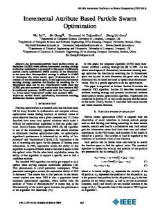
Figure 1. The Geforce 8800 Architecture

memory. A GPU is inherently good at processing a large amount of data in parallel. Each individual processor on the GPU processes a small part of data thereby increasing computing output. Another reason why the GPU is so fast is because of its extremely high memory bandwidth. GPU memory bandwidth is still several times higher than main memory bandwidth. To put it in numbers, a DDR3 1333Mhz system memory has a bandwidth of 32GBps (Gigabytes per second), the corresponding bandwidth of a GeForce 590 GTX is 328 GBps[2]. Such a huge difference has indeed shifted the paradigm of high performance from the CPU to GPU. While sequential part is optimally executed on the CPU, their parallel counterparts would be able to take advantage if the GPUs processing capabilities. In 2007 NVIDIA introduced CUDA programming model designed to implement joint CPU/GPU execution of a program. Following its inception several fields have witnessed benefits of reduced execution time. Some of the examples are SETI and protein folding. In this paper we have presented a CUDA implementation of a global optimization algorithm called Particle Swarm Optimization. An attempt to port this algorithm to CUDA has been previously presented by [3]. We present our implementation exclusive to geophysical application like inversion of potential field and resistivity data.


II. CUDA C++/C PROGRAMMING PARADIGM While parallel processing basically entails distribution of job to several nodes, it’s the programming model that dictates how it is done. CUDA C/C++ consists of 2 kinds of functions. 1. Host Functions, which are executed in the CPU and are sequential in nature. 2. Kernel Functions, which are executed on the GPU in parallel. The kernel functions are further divided into two types 1. __global__ prefixed functions are kernel functions that are called from the CPU and are executed on the GPU. 2. __device__ prefixed functions are kernel functions which are called only from __global__ functions and are executed on the GPU. NVIDIA GPUs employs the Single Instruction Multiple Data (SIMD) concept. This means each processor in a GPU processes the same instruction but to different data sets. This automatically allows faster execution on huge data sets. The SIMD paradigm is implemented in CUDA with the concept of threads, blocks and grids. At the rudimentary level threads refer to a single instruction while block refers to a collection of threads and a grid refers to a collection of blocks. This significance of threads, blocks and grids is that they are processed in different parts of GPU. While a block is executed in a core, a grid is executed in the entire GPU. Using optimal values for them is important to always feed all the GPU processors with data so that no processor remains idle. In most cases these parameters depends on the number of processors that a GPU have. A specific thread and block is referred with the index specifier keyword threadIdx and blockIdx respectively [4]. Every kernel function called from the GPU spawns out a number of user specified thread and block structure and each thread works on a small part of the computation. The variables blockDim and gridDim define the number of threads per block and the number of blocks per respectively [5]. These variables help locate the exact thread in any block or grid. To summarize the optimum procedure of writing a parallel program is send data to GPU to do some extensive work and retrieve data back from the GPU to the CPU. This CPU-GPU transfer is the slowest link of the CUDA programming chain and should be kept to a minimum wherever possible. An overview of the Geforce 8800 Architecture is shown in Figure 1. III.

PARTICLE SWARM OPTIMIZATION

PSO is a global optimization algorithm introduced by Kennedy and Eberhart [6] which simulates the behavior of bird swarms. Lets us suppose a swarm of birds searching for food in a given area. The main motive of the flock is to locate a food source in their environment. In the process of finding the food, each bird knows the position of its nearest approach to the food source. Also the bird closest to the food, passes its position information to all the other birds in the flock. With the knowledge of both, the personal best position and the best position of the flock, each bird updates its position and hence they reach to the food in by spending minimum possible time and energy.

The computational technique of PSO technique is analogous to the behavior of the flock described above. The particles are compared with individual birds, the search space with the environment and the food source with the global minima. All of particles have fitness values which are evaluated by the fitness function to be optimized, and have velocities which direct the direction of movement the particles. PSO is initialized with a group of random particles in an M-dimensional space, with the ith particle represented by m i =

( m , m , . . . , m ) . Each particle maintains 1 i

2 i

M i

1

2

memory of its best position, p i = (p i , p i , . . . , p i ) and N

( v , v , . . . , v ) . At the end of every 1 i

velocity, v i =

2 i

N i

iteration, the particles update their velocity by considering the two best values, i.e. the previous best position occupied by the particle and the best position of the swarm. The new velocity is then used to update the position of each particle. The best position of each particle is termed as pbest and the second best is termed as gbest as it represents the best position of the swarm. The following equations are used for updating the particles:

vik = vik−1 + b ran(.) ( pbesti – mik ) + c ran(.) ( gbest – mik )

(1)

and mi k +1 = mi k + av i k (2) In the above equations, the current location and velocity th th k k of the i particle at the k iteration are mi and vi , respectively, and the best location achieved by the particle so far is pbesti. Further, consider that the best location achieved th by the swarm prior to the k iteration is gbest. Then the new location of the i

th

th

particle in the ( k + 1) iteration is given

by the above two equations. In the velocity equation, it can be noticed that there are three components. The first component is associated with the inertia, second with the personal previous best and is termed as cognitive part and the last one is the social part, associated with the best particle of the swarm. The constant b and c are represented as the learning rates, governing the cognition and social part respectively. The other constant a is a constriction factor introduced by [7] to dynamically lower the velocities as time progresses, gradually focusing on a local search. The values of the constant b and c are empirically determined but in general their sum is equal to four. They are defined for a problem in such a way that it makes the algorithm best suited for that problem. The ran (.) function denotes a random number in the interval (0, 1). While updating the velocity and the position of the particle, a constraint that the location of each particle should not exceed the boundaries of the given search space of that parameter. To apply this constraint, the velocity of the


particle is reversed as required. To implement the serial version of the above described algorithm, following pseudo code can be used. 1. 2. 3. 4. 5. 6. 7.

Initialize Particles. Evaluate each particle to find pbesti and gbest. Start Iteration. Modify Velocity and equation for each particle using equation 1 and 2. If a better solution is obtained update pbesti and gbest. End iteration. Output the best Solution.

A. Cuda Implementation of Standard PSO By studying the pseudo code we can very well see that steps 1,2,4 and 5 can be inherently parallelized where each thread calculates for individual particles. The function corresponding to those steps have been taken as kernel functions which are executed on the GPU. The pseudo code of the CUDA version takes some modifications to the serial version and is outlined below.

1. 2. 3. 4.

5. 6. 7.

Initialize Particles on the GPU where each thread initializes a particle. Evaluate each particle in parallel to find pbesti and gbest. Start Iteration. Modify Velocity and equation for each particle in individual threads using equation 1 and 2. If a better solution is obtained update pbesti and gbest. End iteration. Output the best Solution.

The steps 1, 2, 4 and 5 have been modified to be executed on the GPU and thereby reaping benefits of a reduced execution time. A 64-bit random number generator was used to generate random numbers in the interval (0, 1). IV.

RESULTS AND DISCUSSIONS

A. The Testbed Our test setup consisted of a HP laptop with a Intel Core2Duo T5800 running at 2GHz with 3 GB of 800MHz DDR2 RAM. The GPU was a NVIDIA 9200M GS having 8 CUDA cores. The setup was running UBUNTU 32-bit version 10.04 running CUDA TOOLKIT 3.2. GCC version 4.3.3 was used as the preferred C compiler. The X-server was shutdown in all cases so that GPU is free from any kind of load arising from rendering the GUI of the OS. This is also done due the fact that a GPU connected to a display device is not allow to execute a kernel function for more than 5 seconds.

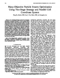
Figure 2. Speed comparison of CUDA PSO and CPU PSO

B. Speed up Demonstration T o d e mo nstr a te the a c c e le r a tio n ob ta ine d b y implementing CUDA we compared our implementation with a very efficient single core CPU version of the same algorithm. This algorithm was then tested on different kinds Table I: Comparison of Runtimes of the CUDA and the CPU version with the Corresponding Speedup

No of Particles 256 384 512 768 1024

Runtime (msec) CUDA PSO CPU PSO 2549 36592 3370 54912 3688 73193 4904 109679 6263 140377

Speed Up 14.35 16.29 19.84 22.36 22.41

of geophysical data to show its feasibility. The speed up was measured by dividing the time taken to execute the CPU version with the CPU version with the number of iterations being fixed at 1000. We compared the speed up for different population size and the saw an increasing trend till 768 particles after which there was saturation. The runtime values for different population size for the algorithms are tabulated in table I. The corresponding graphical variation of the speed up is demonstrated in Figure 2. This is attributed to the fact that as the number of particles increase they can’t be processed at once in the GPU and has to be sent in two cycles thereby nullifying the speed gain. Still it’s a remarkable observation as to how we are getting a minimum speed up of 17x – 22x using CUDA. Moreover to show that the CUDA version is as accurate as the original serial version we compared the model parameters and response curve of their results side by side with the search space for each parameter mentioned within square brackets.

C. Self Potential Data The Self Potential (SP) refers to the spontaneous potential that arises due to various electrochemical mechanisms and sometimes it may also develop due to human disturbance of the environment like buried electrical


cables, drainage pipes or waste disposal sites. Such potential ranges from a fraction of milivolts(mV) to hundreds of mV as in the case of sulphide and graphite ore bodies. Some of the dominant mechanism that leads to such spontaneous potential can be attributed to processes like electro filtration or mineral potential. The self potential response due to a buried body is given by the equation

(3) Where x is the horizontal distance on the surface, x0 denotes the position of source in horizontal axis, z represents the depth of the source and θ defines the angle of polarization of the source. K is the dipole moment while q is the shape factor of the source taking values of 0.5, 1.0 and 1.5 for a vertical cylinder, horizontal cylinder and sphere respectively. And the Self Potential response due to a buried sheet is given by

(4) Where θ is the inclination angle, a is the half width of the sheet, x0 is the horizontal position centre of the sheet and z is the depth. Table II: Model Parameters of the Surda SP anomaly

Source 1

Parameters K [90 to180] X0(m) [-20 to 40] Z(m) [10 to 40] A(m) [10 to 30] È(degrees) [20 to 50]

CUDA PSO 99 -2.08 31.06 26.57 46.10

CPU PSO 98.2 -1.21 30.9 27.3 45.1

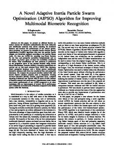
We have selected an anomaly over Surda Area of Jharkhand, India. The causative source of this anomaly is attributed to an inclined sheet whose parameters have been obtained by inverting the response according to equation 4.The parameters obtained from both the CUDA and CPU version are listed in table II. The corresponding plot of the responses is shown in Figure 3.

D. Magnetic Data Magnetic anomalies observed over the earth can be attributed to magnetic susceptibility contrasts in the underlying rocks. Magnetic anomalies are used to delineate several features like buried ores, contacts and basement depths. We have adopted the analytic signal approach to interpret the data [8]. The forward modeling equation can be approximated using the equation

A( x) =

K 2

2

q

(5)

[( x − x0 ) +( z) ]

Where K is the amplitude factor related to the physical properties of the source, x0 and z0 are the horizontal location and depth of the source, respectively, and q is known as shape factor. A term, structural index (SI) defined by 2q1takes values 0, 1 and 2 for magnetic anomalies over a contact, a thin dyke and a horizontal cylinder, respectively corresponding to shape factors 0.5, 1.0 and 1.5, respectively. We consider the amplitude of the vertical magnetic anomaly of Boston Township, Ontario, Canada [9]. This anomaly is more than four times the intensity of the Earth’s magnetic field. The analytic signal shows 2 distinct peaks which have been delineated by PSO. The inverted parameters from the two versions of the algorithms are shown in Figure 4 and their corresponding parameters are tabulated in table III. The results delineate an ambiguous source (SI=1.6) and a horizontal cylinder Table III: Model Parameters of Boston Magnetic Anomaly

Parameters

CUDA PSO

CPU PSO

K [10 to1000] X0(m) [12 - 24] Z(m) [1 to 25] 2Q-1 [0.2- 2.5]

8781 19.8 7.5 1.6

8788 19.8 7.6 1.6

K [10-1000] X0(m) [12- 36] Z(m) [1-25] 2Q-1 [0.2- 2.5]

9721 27.7 3.7 1.96

9745 27.8 3.6 1.96

Bell 1

Bell 2

Figure 3. Graphical Response of the field data and the inverted model for Surda SP data.


ρ a (ohm-m) [25 to

40.25

40.17

1.81

1.79

100.9

101.2

11.27

11.15

11.53

11.47

60] Depth (m) [1 to 2.2] Layer 2

ρ a (ohm-m) [75 to 180] Depth (m)[4 to 12] Layer 3

ρ a (ohm-m) [7 to 20] Figure 1. Graphical Response of the field and the inverted model for Boston area.

V. CONCLUSIONS We have demonstrated the benefits of reduced execution time in case of CUDA PSO over a serial PSO. Moreover the model parameters calculated by both the algorithms show no ambiguity in any case. It should be considered that our test bed had the weakest GPU in the NVIDIA's portfolio. A speed up of about 22x over this card would correspond to a even higher value with a better GPU. Finally we conclude that the CUDA implemented algorithms in the geophysical domain can show rich benefits of reduced computing time and accurate results at the same time. ACKNOWLEDGMENT The authors are grateful to the Director, NGRI for giving all the necessary support for this work.

Figure 2. Graphical Response of the field and the inverted model for Satkui Data

(SI=1.96) at the two bells respectively. This was further substantiated with the help of drill hole results.

E. Resistivity Data We follow [10] and write the expression for the apparent resistivity measured with a Schlumberger array over a multilayered 1D earth model as ∞

ρ a ( r ) = r ∫ T (λ ) J1 ( r λ )λ d λ 2

(6)

0

and

Where r is half of the current electrode spacing (AB/2), J1 (λ r ) is the Bessel function of the first order and

T (λ ) is the resistivity transform.. We have taken a field case from Satkui after [11] and inverted the data for 3 layers. The model parameters will be tabulated in table 3 and the corresponding plots are shown in Figure 3. Table IV: Model Parameters of Satkui Resistivity Data

Parameters Layer 1

CUDA PSO

CPU PSO

REFERENCES [1] [2] [3]

GPGPU homepage http://gpgpu.org NVIDIA homepage http://nvidia.com Lucas de P. Veronese, and Renato A. Krohling, 2009, IEEE Congress on Evolutionary Computation (CEC 2009), 3265-3270.. [4] NVIDIA, CUDA 2.0 Programming Guide,http:// developer.download. nvidia.com/compute/cuda/2_0/docs/NVIDIA_CUDA_Programming_ Guide_2.0.pdf. [5] NVIDIA,CUDA documentation,http://www.nvidia.com/object/cuda_develop.html. [6] Kennedy, J., and R. Eberhart, 1995, Particle swarm optimization: Proceedings of the IEEE International Conference on Neural Networks, IV, 1942–1948.Electronic Publication: Digital Object Identifiers (DOIs): [7] Clerc, M., 1999, The swarm and the queen: Towards a deterministic and adaptive particle swarm optimization: Proceedings of the IEEE Congress on Evolutionary Computation, 1951–1957. [8] Nabighian, M.N., 1972. The analytic signal of two-dimensional magnetic bodies with polygonal cross-section: its properties and use for automated anomaly interpretation, Geophysics, 37, 507–517 [9] Shalivahan Srivastava and B. N. P. Agarwal, 2010, Inversion of the amplitude of the two-dimensional analytic signal of the magnetic anomaly by the particle swarm optimization technique, Geophys. J. Int. (2010) 182, 652–662. [10] Koefoed, O., 1979, Geosounding principles, 1: Resistivity sounding measurements:Elsevier Scientific Publishing Company. [11] Sankar Kumar Nath, Shamsuddin Shahid, Pawan Dewangan, 2000, SEISRES Ð a Visual C++ program for the sequential inversion of seismic refraction and geoelectric data, Computers & Geosciences 26 (2000) 177-200.