TEM Journal 5(2) 152–159
CUDA Based Speed Optimization of the PCA Algorithm Salih Görgünoğlu 1, Kadriye Öz 2, Abdullah Çavuşoğlu 3 1
2
Karabük University,Department of Computer Engineering,Karabük, Turkey Karabük University,Department of Electronics and Computer Education,Karabük, Turkey 3 Council of Higher Education,Higher Education Committee, Ankara, Turkey
Abstract –Principal Component Analysis (PCA) is an algorithm involving heavy mathematical operations with matrices. The data extracted from the face images are usually very large and to process this data is time consuming. To reduce the execution time of these operations, parallel programming techniques are used. CUDA is a multipurpose parallel programming architecture supported by graphics cards. In this study we have implemented the PCA algorithm using both the classical programming approach and CUDA based implementation using different configurations. The algorithm is subdivided into its constituent calculation steps and evaluated for the positive effects of parallelization on each step. Therefore, the parts of the algorithm that cannot be improved by parallelization are identified. On the other hand, it is also shown that, with CUDA based approach dramatic improvements in the overall performance of the algorithm are possible. Keywords – Principal Component Analysis, CUDA, Parallel Programming, Parallel GPU Computing.
1. Introduction Face recognition involves comparison of the face(s) -extracted either from a static or video imagewith the faces in the database [1,2]. Obviously, successful matching is the main goal here. This operation is required in the case of ID determination and verification. Principal components analysis is a statistical method used for reducing the size of data. The eigenface method has been developed by Turk and
DOI: 10.18421/TEM52-05 https://dx.doi.org/10.18421/TEM52-05 Corresponding author: Kadriye Öz - Karabük University, Department of Electronics and Computer Education, Karabük, Turkey Email:
[email protected] © 2016 Kadriye Öz et al, published by UIKTEN. This work is licensed under the Creative Commons AttributionNonCommercial-NoDerivs 3.0 License. The article is published with Open Access at www.temjournal.com
152
Pentland in 1991 [3]. The eigenface approach since has been used as the base for several studies [4-6]. In the literature, to improve the success rate of face recognition and of the PCA algorithm, many algorithms such as Radial Basis Function Network (RBF) and Linear Discriminant Analysis have been developed [7,8]. In the studies involving face recognition, the resolution of the images has an important effect on the possible operations that is required. The approaches/methods used in problem solving, usually reduces the size of data without losing the valuable information. Search for faster/better techniques is still continuing. GPU based general purpose programming has recently become so popular because of the possible performance improvements in the algorithms otherwise executed on the main processors. There are 3 main Technologies in this field [9]. Advanced Micro Devices (AMD) has introduced the BROOK+ technology [10]. While the Khronos Group has developed the Open Computing Language (OpenCL) [11]. Compute Unified Device Architecture (CUDA) is, on the other hand, a general purpose parallel programming architecture presented by NVIDIA[12]. Because of its versatility and multipurpose structure CUDA has been used in many applications for improving the performance. For example in a survey, Luebke points out that CUDA based processing speedups in several areas including chemistry, astrophysics, CT, MRI and gene sequencing and obtained speed, increase between the ranges of 10× to 100× [13]. Especially computations involving heavy matrix operations are very suitable to be executed in parallel using CUDA [14,15]. The algorithm that is used often have also benefited from this parallel programming technique, for example it is used for speeding up the K-Means algorithm with GPU [16]. In some applications such as “the numerical solution of two-layer shallow water systems”, CUDA has been used with MPI and the performance improvement of the system is targeted [17]. In another study, CUDA and OpenCL have been used together to find out parallel programming performances of different graphics cards [18]. Also, effectiveness of the CUDA programming language
TEM Journal – Volume 5 / Number 2 / 2016.
TEM Journal 5(2) 152–159
has been evaluated taking into account both the advantageous and disadvantageous sides of it [19]. Another programming language that may be used in CUDA architecture programming is CUDA C. In this environment to facilitate programming some library functions have been incorporated [20,21]. Another utility program is called Auto Parallelizing Translator from C to CUDA (APTCC) [22] and aims to translate the C code to CUDA C -without any compiler directives- isolating the user from the complicated GPU architecture and directly focusing to the algorithm. In the following section we re-visit some of the technical issues of CUDA. Afterwards, in section 3 the details of parallelization of the PCA algorithm using CUDA aregiven. Section 4 is about discussion and evaluation of improving the performance of PCA using CUDA. Finally, section 5 concludes this paper. 2. Technical Application Details Using CUDA The CUDA parallel programming model has been constructed to help the users who are familiar with the standard C programming. It has been presented to the programmers with 3 main basic issues: the thread hierarchy, shared memories and barrier synchronization, with little extensions to programming languages. In CUDA programming model, the main processor (CPU) is named as host to the GPU and facilitating to the CPU is called device. The function to be executed by the device is called kernel and identified with “__global__” prefix, and is shown in Algorithm 1. Algorithm 1: The definition of the device and funtion to be executed by the device. 1. __global__ void calculateA(float* d_A,float* d_face, float* d_meanface, int facecount,int pixel) 2. { 3. int i=threadIdx.x; 4. int j = blockIdx.x; 5. d_A[index] = d_face[index] - d_meanface[j]; 6. } int index=i+j*facecount; 7.
The GPU memory is also managed by the host. The host initially allocates memory for the data to be used by the device and copies this data to this section as shown in Algorithm 2. Algorithm 2: Memory allocation on the device and copying the data to this memory space. 1. unsigned int size_face = faceCount * pixel; 2. unsigned int mem_size_face = sizeof(float) * size_face; 3. unsigned int mem_size_meanface = sizeof(float) *pixel; 4. float* d_A;
TEM Journal – Volume 5 / Number 2 / 2016.
5. 6. 7.
float* d_face; float* d_meanface; cutilSafeCall(cudaMalloc((void**) &d_A, mem_size_face)); 8. cutilSafeCall(cudaMalloc((void**) &d_face, mem_size_face)); 9. cutilSafeCall(cudaMalloc((void**) &d_meanface, mem_size_meanface)); 10. cutilSafeCall(cudaMemcpy(d_face,face, mem_size_face, cudaMemcpyHostToDevice) ); 11. cutilSafeCall(cudaMemcpy(d_meanface,meanface, mem_size_meanface, cudaMemcpyHostToDevice) );
The host must also determine the grid and block size and adjust the kernels execution. When the kernel finishes its work, as illustrated in Algorithm 3, the host transfers the data from the device memory into the host (i.e. the main) memory. Afterwards, the host should also free the memory allocated on the device. The kernel is called by the host using: KernelName(…) is executed by a number of threads run parallel on the device. Although all the threads execute the same code, using their unique threadId they behave differently when taking decisions, making computations and accessing the memory. Algorithm 3: Execution of the codes on the device, transferring the results back to the host and freeing the spaces on the device. 1. int block =pixel; 2. int thread=faceCount; 3. calculateA >(d_A,d_face,d_meanface,faceCount,pixel); 4. cudaThreadSynchronize(); 5. cutilSafeCall(cudaMemcpy(A, d_A, mem_size_face,cudaMemcpyDeviceToHost) ); 6. cutilSafeCall(cudaFree(d_A)); 7. cutilSafeCall(cudaFree(d_face)); 8. cutilSafeCall(cudaFree(d_meanface));
ThreadID gives us the index of a thread in a certain block. It can be 1,2 or 3 dimensional. In a one dimensional block, thread ID is the dimension index while in a 2 dimensional block (i.e. Dx, Dy) the thread index becomes (x + y Dx ); and in 3 dimensions (i.e. Dx, Dy, Dz) ) the thread index becomes (x + y Dx +z DxDy ). Block index in a grid is represented as blockID and it can be one or two dimensional. These values could be accessed using blockIdx.x and blockIdx.y. The number of therads in a block can be expressed with blockDim as 1,2 or 3 dimensional. This value is 512 for the GPUs having compute capacity 1.x while it is 1024 for the GPUs with the compute capacity 2.x. The maximum number of blocks in a grid could be 65535 and is expressed with gridDim as 1 or 2 dimensional. In figure 1., block structure in a grid along with the thread structure is shown.
153
TEM Journal 5(2) 152–159
Figure1. The diagram for a grid of thread blocks
In CUDA programming model, each thread has its own local memory. In addition, all threads in the same block can access the shared memory space while the global device memory is used for the communication between the host and the device. This is accessible to all threads in the GPU. The constant and texture memory is accessible by the host for both read/write modes, while the threads in the GPU can only access theread mode. The CUDA device memory space diagram is shown in figure 2. Block[0,0]
Block[1,0]
Shared Memory
Shared Memory
Registers
Thread[0,0]
Registers
Registers
Thread[1,0]
Thread[0,0]
training set images with the highest variance are selected and their projections onto the relevant dimension are taken. Each of these dimensions is called eigenfaces. Taking the projection means that the representation of the face as the sum of weights of eigenfaces [23]. The PCA consists of 2 stages: training and recognition. Here the aim is calculating the covariance vector representing the face distribution and finding the eigenvectors [24]. The eigenvectors may be regarded as representation of differences between the faces. In the training dataset, there is an eigenvector for each face. However, in the recognition stage the eigenvectors with highest values (i.e. the ones contributing the highest value to the distribution) are selected and used. In the recognition stage, a threshold value is used for comparison. The PCA algorithm consists of the steps given in table 1. and table 2. [3, 24]. In table 1., the feature extraction steps are given. While in table 2. the steps for recognition of a given face by the PCA algorithm are given. Table 1.Calculation Steps Of Feature Extraction Using The PCA Algoritm Algorithm
Description
x'=
Normalization
Registers
Thread[1,0]
Mean Calculation Local Memory
Local Memory
Local Memory
x − min A max A − min A
Ψ=
1 M
M
∑Γ n =1
n
Local Memory
Global Memory Host (CPU) Constant Memory
Φ calculation
Φ i = Γi − Ψ
A Transpose Calculation
AT
L Calculation
L = AT A
Eigenvector Calculation
L .v= λv
Eigenface Calculation
𝑢𝑢𝑙𝑙 = � 𝑣𝑣𝑙𝑙𝑙𝑙 Φ𝑘𝑘
Texture Memory
Figure 2.Device memory space diagram for CUDA [16].
3. Parallelization of PCA using CUDA As mentioned earlier, the PCA is a statistical method employed when the evaluated data is too big. It’s based on reduction of this data and interpretation of it. Turk and Pentland [3] have applied this approach to face recognition algorithm and developed the well known Eigenfaces method. In this method,
154
Feature Calculation
𝑀𝑀
Vector
𝑘𝑘=1
𝑙𝑙 = 1, … . , 𝑀𝑀
wk = u kT (Γ − Ψ )
Explanation x represents the color value of a pixel in the image, min A represents the smallest color value in the face (i.e. image), max A represents the biggest color value in the face (i.e. image), Γ 1 , Γ 2 .. Γ M column matris corresponding to each face in the training set, if the size of the face image is NxN then each column matris Γ will have the size N2x1, M number of faces in the training set, Ψ mean value of the set Φ i the difference of the face from the mean value, A=[ Φ 1 ,Φ 2 ,Φ 3 ...,Φ M ], Φ i fort he size N2x1, The A matris size becomes N2xM, L reduced matris (sizewise) calculated instead of covariance matris, multiplication of MxN2 with N2xM sized matris produces MxM sized matris, v is eigenvector and λ is eigenvalue U is eigenface,
W is the feature vector
TEM Journal – Volume 5 / Number 2 / 2016.
TEM Journal 5(2) 152–159 Table 2. Calculation Steps Of Face Recognition Using The PCA Algoritm Algorithm
Description
x − min A max A − min A
Normalization
x'=
Difference from mean
Φ T = ΓT − Ψ
Feature vector extraction
wt = U .Φ T M
Distance control
d i = ∑ wT ( j ) − wi ( j ) j =1
i = 1,2,...N
Explanation the color values of the face to be recognized normalized to between 01, its difference from the mean face is calculated The feature vector is calculated using the eigenvectors, The distance between the feature vectors are calculated for a successful matching,
4. Discussion and Evaluation of the Established Improvements of the Performance of PCA with CUDA
speedup =
TimeCPU TimeGPU
(1)
In this equation TimeCPU and andTimeGPU correspond to the times spend by the main CPU of the system and the graphics processor located on the graphics cards respectively. CUDA based speedup rates for PCA algorithm has been obtained over the ORL face database [25]. This database contains 400 images of 92x112 resolutions belonging to 40 different individuals. In the min-max normalization stage, each thread travels through the pixels that form a face image and finds the minimum and maximum values of them. The same thread makes a second traversing operation on them but this time to normalize the values within the range of 0-1. As figure 3. illustrates for 400 face images, speedup rates of up to 5-6 times are obtained.
In our application we have executed the PCA algorithm on 3 different Graphics Cards on the same computer configuration. The base configuration used as a testbed has Intel Core I3 550 3.2 GHz CPU, 4 GB DDR3 1333 MHz RAM, Microsoft Windows 7 Professional (x64) O/S. The performance values that are obtained for the algorithm along with the hardware specifications of graphics cards are listed in table 3. Table 3.The specification of graphics cards used in PCA computations. Figure 3. Speedup rates for the normalization algorithm Core Number Compute Capability Streaming Multiprocessors Max threads per blocks Clock rate
GeForce GT220 48 1.2
GeForce GeForce GT630 450 96 192 2.1 2.1
6
2
4
512
1024
1024
1012000
1620000
118900
The face recognition accomplished using the PCA algorithm consisted of several computations (e.g. as listed in table 1. and table 2.). The CPU and GPU execution times and speed up ratios are shown with a number of figures (i.e. figure 6. and figure 12.).
As Figure 4. illustrates, for the calculation of means of 400 face images, speedup rates of 2.5-3.5 have been obtained. To transfer the data (i.e. out of 400 images) from host to device and from device to host was 6.53 ms for the GTS 450 graphics card, while the time elapsed on the GPU for means calculation was 10.15 ms, totaling up to 16.68 ms. While the CPU time for the same process is 35.57 ms. Comparison of the total times for GPU and CPU clearly shows the benefit of GPU programming.
In the calculation of speedup rates for the PCA algorithm, the steps that are listed in table 1. and table 2. are executed 10 times, the elapsed times are added and divided by 10 to find the mean value of the time spent for each step (i.e. due to different tasks which may affect the overall execution time). The mean TimeCPU and TimeGPU values are calculated by this method. Afterwards, using these values, speedup is calculated as below. Figure 4.Speedup rate for the calculation of means.
TEM Journal – Volume 5 / Number 2 / 2016.
155
TEM Journal 5(2) 152–159
In figure 5., the Φ calculation for 400 images is shown. As it may be observed from the figure, for 400 images, speedups of 4 times (i.e. approximately) are obtained. However, around 320 images of the maximum speedups (i.e. up to 12 times) are recorded. This is due to the exact conformity between the number of cores and the number of threads when the divisions are made. Similar to the means calculation, to transfer the data from host to device and from device to host was 18.98 milliseconds for the GTS 450 graphics card, while the time elapsed on the GPU for means calculation was 1.66 ms, totaling up to 20.64 ms. While the CPU time for the same process is 83.90 ms. Again the benefit of parallel programming over the GPU is crystal clear.
Figure 5. Speedup rate of Φ calculation
Figure 6. shows the speedups obtained for the transpose operations. This time, the speedup factor is 2 times. For the same graphics card the data transfer time is 16.69 and transpose operations on the GPU costs 12.15 ms totaling up to 28.84 ms.While the CPU time for the same process is 67.10 ms.
Algorithm 4: Calculating L=ATxA on CPU // faceCount:the number of face image ; // pixel: the pixel number of a face image; for i←0 to faceCount for j←0 to faceCount for k←0 to pixel L[i, j] ←. L[i, j] +ATranpose[i, k] * A[k, j]; end of for; end of for;
Algorithm 5: Calculating L=ATxA based on the register of the GPU // threadDim: the dimension of the thread in each block; // blockDim: the dimension of the block in each grid; // blockIdx.x: the current block ID; // threadIdx.x: the current thread ID; // faceCount:the number of face image ; // pixel: the pixel number of a face image; //index: the adress of data which willl be calculated //aindex: index which will be used in multiplication //aTIndex: index of the cell in transpose matrix( AT) which will be used in multiplication 1. index=blockIdx.x*faceCount+threadIdx.x; 2. for j=0 to pixel 3. aIndex←blockIdx.x*pixel+j; 4. aTIndex←j*faceCount+threadIdx.x; 5. sum←sum+ A[aIndex]*d_AT [aTIndex]; 6. end of for; 7. L[index]← sum;
As figure 7. illustrates, the calculation of covariance in the eigenface algorithm is the most time consuming part when the overall algorithm is considered. For this part, speed up rates ranging between 25-212 have been obtained. As figure 7. clearly illustrates, the increase on the number of core in the graphics processor has a dramatic effect on the performance of this section of the algorithm. In addition, increasing the number of faces does not cause much negatives on the performance.
Figure 6. Speedup rate for calculation of transposes.
In terms of calculation times the most time consuming algorithms are L, U and W. The nature of these calculations are very similar. Therefore, GPU and CPU times for L has been shown as an example for the algorithms 4 and 5.
156
Figure 7. Speedup rates of L calculation
TEM Journal – Volume 5 / Number 2 / 2016.
TEM Journal 5(2) 152–159
As figure 8. illustrates, in the calculation of eigenfaces speedup values up to 15-80 times have been obtained. For 400 images the CPU calculation time is 5584.81 ms while the GPU time for GTS 450 graphics card is 69.49 ms.
Figure 8.Speedup rate of Eigenface (U) calculation
As figure 9. illustrates, when calculating the eigenfaces, speedup values up to 5-185 times are observed. For 400 images, the CPU calculation time is 7099 ms while the GPU time for GTS 450 graphics card is 36.26 ms.
stages of the algorithm. These 4 stages of the algorithm consume 321.84 ms. The total CPU time for the overall algorithm is 48446.49 ms. Compared to the overall algorithm’s time, the consumed time for these 4 operations is about 0.6%. Therefore, the effect of these parts is limited. On the other hand, the overall speedup rate for the PCA algorithm is 139.69 times. On the other hand, as table 3. illustrates, (i.e. considering the 4 stages of the algorithm mentioned above) although the GT220 has 48 cores (i.e. lesser number of cores when compared to GT 630 and GTS 450), its performance is still nearer to the other cards with higher number of cores (e.g. table 4., the transpose calculations). This is due to the higher number of streaming processors (SMs) employed in this GPU (i.e. as shown in table 3.). This is because the SMs are used to process higher number of blocks at the same time. If the processed data contains big sized data blocks, the lesser number of blocks is not a disadvantage, however in the cases where the data block sizes are small, the tasks performed by the SMs is higher. Therefore, this also has a reflection on the performance of the GPUs in parallel processing applications. Table 4. Time analysis for 400 images .
Figure 9. Speedup rate of feature vector (W) calculation
In table 4. CPU timings corresponding to the GTS450 are shown. In addition the timings corresponding to the same system using 3 different graphic cards has been given. The maximum speedup rate has been obtained for L, U and W reaching up to 212, 80 and 195 respectively. While the minimum speedup rate was found for Transpose calculation as 2.32 times. In the calculations of normalization, mean, Φ(A) and transpose operations, the obtained speedup factors are relatively low when compared to the other
TEM Journal – Volume 5 / Number 2 / 2016.
Algorithms
CPU Time (ms)
GPU Time (GT 220) (ms)
GPU Time (GT 630) (ms)
GPU Time (GTS 450) (ms)
Normalization
135.27
29.60
21.89 24.26
5.57
Mean calculation
35.57
13.17
12.65 11.02
3.22
Φ(A) calculation
83.90
23.07
20.51 20.64
4.06
A Transpose calculation
67.10
27.62
30.14 28.84
2.32
L calculation
35576.11 442.28
237.0 167.30 0
212.6 4
U calculation
5584.81
105.86
69.23 69.49
80.36
W calculation
7099.00
101.45
50.05 36.26
195.7 8
Overall
48446.49 743.05
428.8 346.79 2
139.6 9
Speed Up*
*The values correspond to this configuration with the GTS 450 graphics card.
157
TEM Journal 5(2) 152–159
5. Conclusion
The PCA algorithm is a widely used technique used in many different fields as well as face recognition, which was the subject of this study. The algorithm is employed especially in the cases where the data sets are too big and their reduction for feature extraction without losing the meaningful information is the case. Despite this fact that the algorithm contains heavy mathematical computations, parallel programming, especially the usage of the sources on the graphics cards for this purpose (e.g. CUDA based programming), has become popular among the scientist who are seeking performance improvements over several such applications containing dense arithmetical operations. Obviously, parallel programming provides a certain amount of improvements in any application when compared to the traditional techniques. However, breaking a complex algorithm and evaluating the constituent parts of the algorithm separately gives us a clearer picture. On the one hand, one can examine the theoretically based possible improvements of the parallelism at work; while on the other hand, the possibility of improvements and focus on different sections of the algorithm may be possible. While showing the performance/improvement of the speed on PCA algorithm using the CUDA, we have also illustrated the problematic sections of the algorithm with this regard. We believe that this will open a field for the researchers who work on the improvement of this kind of algorithms. Acknowledgements This work is supported by Karabük University research fund under Grant no KBÜ-BAB-11/2-YL036. References [1] Tolba A.S., El-Baz A.H., El-Harby A.A. (2005). Face recognition: a literature review.International Journal of Signal Processing. 2(2), 88-103. [2] Tan X., Chen S., Zhou Z., Zhang F. (2006). Face recognition from a single image per person: A survey.Pattern Recognition. 39, 1725-1745. [3] Turk M., Pentland A. (1991). Eigenfaces for recognition. Journal of Cognitive Neuroscience. 3, 71-86. [4] Zhang D., Zhou Z. (2005). (2D)2PCA: Twodirectional two-dimensional PCA for efficient face representation and recognition.Neurocomputing. 69, 224-231. [5] Eftekhari A., Forouzanfar M., Moghaddam H.A.,Alirezaie J. (2010). Block-wise 2D kernel PCA/LDA for face recognition.Information Processing Letters. 110, 761-766.
158
[6] Kusuma G.P., Chua C.S. (2011). PCA-based image recombination for multimodal 2D+3D face recognition. Image and Vision Computing. 29, 306316. [7] VirginiaE.D. (2000).Biometric Identification System Using a Radial Basis Function Network, Proc 34nd Annual IEEE In!. Carnahan Conf. on Security Technology. 47-51. [8] Lu J., Kostantinos N.P., Anastasios N.V. (2003). Face recognition using LDA-based algorithm.IEEE Trans.Neural Networks. 14, 195-200. [9] Riha L.,& Smid R. (2011).Acceleration of acoustic emission signal processing algorithms using CUDA standard.Computer Standards & Interfaces. 33, 389400. [10] Advanced Micro Devices Inc.(2009). Ati stream computing technical overview. http://developer.amd.com/gpu_assets/Stream_Comput ing_Overview.pdf. [11] Munshi A.(2009). TheOpenCL specification version 1.0, Khronos Group, Beaverton, OR. [12] NVIDIA Corp. (2014). CUDA C Programming Guide. http://docs.nvidia.com/cuda/pdf/CUDA_C_Programm ing_Guide.pdf. [13] LuebkeD. (2008). Cuda: Scalable parallel programming for high-performance scientific computing.Biomedical Imaging: From Nano to Macro 5th IEEE International Symposium, Trondheim.838838. [14] Okitsu Y., Ino F., Hagihara K. (2010).Highperformance cone beam reconstruction using CUDA compatible GPUs. ParallelComputing . 36, 129-141. [15] Kalentev O., Rai A., Kemnitz S., Schneider R,. (2011). Connected component labeling on a 2D grid using CUDA.J. Parallel Distrib. Comput. 71, 615620. [16] Li Y., Zhao K., Chu X., Liu J.(2013). Speeding up kMeans algorithm by GPUs. Journal of Computer and System Sciences. 79, 216-229. [17] De la Asunción M., Mantasa J.M., M. J. Castro,Fernández-Nieto E.D. (2012). An MPI-CUDA implementation of an improved Roe method for twolayer shallow water systems. J. Parallel Distrib. Comput. 72, 1065-1072. [18] Du P., Weber R., Luszczek P., Tomov S.,Peterson G., Dongarra J.(2012).From CUDA to OpenCL: Towards a performance-portable solution for multi-platform GPU programming. Parallel Computing . 38, 391407. [19] Che S., Boyer M., Meng J., Tarjan D.,Sheaffer J. W.,Skadron K.(2008).A performance study of general-purpose applications on graphics processors using CUDA. J. Parallel Distrib. Comput. 68, 13701380. [20] Nvidia: cuBLAS Library. http://docs.nvidia.com/cuda/pdf/CUBLAS_Library.pd f. (2014). [21] Nvidia: cuFFT Library User's Guide. http:// http://docs.nvidia.com/cuda/pdf/CUFFT_Library.pdf.( 2014).
TEM Journal – Volume 5 / Number 2 / 2016.
TEM Journal 5(2) 152–159 [22] Nawataand T., Suda R. (2011).APTCC : Auto parallelizing translator from C to CUDA. International Conference on Computational Science, Amsterdam. 352-361. [23] Salah A.A. (2006). İnsan ve Bilgisayarda Yüz Tanıma, Uluslararası Kognitif Nörobilim Sempozyumu, Marmaris, Turkey.
[24] Görgünoğlu S., Öz K., Bayır Ş. (2011).Performance analysis of eigenfaces method in face recognition system. 2nd International Symposium on Computing in Science & Engineering, Aydın, Turkey. 136-142. [25] The ORL Database of Faces: http://www.cl.cam.ac.uk/Research/DTG/attarchive:pu b/data/att_faces.zip.(2014). :
TEM Journal – Volume 5 / Number 2 / 2016.
159