Current noise in a vibrating quantum dot array - DTU Orbit

PHYSICAL REVIEW B 70, 205334 (2004)

Current noise in a vibrating quantum dot array Christian Flindt,1,* Tomáš Novotný,1,2,† and Antti-Pekka Jauho1,‡ 1MIC-Department

of Micro and Nanotechnology, Technical University of Denmark, DTU-Building 345east, DK-2800 Kongens Lyngby, Denmark 2Department of Electronic Structures, Faculty of Mathematics and Physics, Charles University, Ke Karlovu 5, 121 16 Prague, Czech Republic (Received 21 May 2004; published 23 November 2004)

We develop methods for calculating the zero-frequency noise for quantum shuttles, i.e., nanoelectromechanical devices where the mechanical motion is quantized. As a model system we consider a three-dot array, where the internal electronic coherence both complicates and enriches the physics. Two different formulations are presented: (i) quantum regression theorem and (ii) the counting variable approach. It is demonstrated, both analytically and numerically, that the two formulations yield identical results, when the conditions of their respective applicability are fulfilled. We describe the results of extensive numerical calculations for current and current noise (Fano factor), based on a solution of a Markovian generalized master equation. The results for the current and noise are further analyzed in terms of Wigner functions, which help to distinguish different transport regimes (in particular, shuttling versus cotunneling). In the case of weak interdot coupling, the electron transport proceeds via sequential tunneling between neighboring dots. A simple rate equation with the rates calculated analytically from the P共E兲 theory is developed and shown to agree with the full numerics. DOI: 10.1103/PhysRevB.70.205334

PACS number(s): 73.23.Hk, 85.85.⫹j, 72.70.⫹m, 73.63.⫺b

I. INTRODUCTION

As the advances of the technology push the size of the electronic components toward the atomic scale, interesting phenomena influencing the electronic transport emerge. Research fields, e.g., molecular electronics, spintronics, or nanoelectromechanical systems (NEMS) have appeared. A common theme is the combination of quantum transport and a subtle interplay between various degrees of freedom which plays an essential role for the functionality of the device. This paper focuses on the NEMS,1–3 a logical extension of the now established technology of microelectromechanical systems (MEMS), where the electronic (or magnetic) degrees of freedom are coupled to a mechanical degree of freedom. While still in its infancy, NEMS has already attracted much attention both experimentally4–9 and theoretically.10–35 A measurement of the stationary IV-characteristic of a NEMS device does not always yield enough information to uniquely identify the underlying microscopic charge transport mechanism. A point in case is the C60 single electron transistor (SET) experiment by Park et al.5 where two alternative interpretations, namely, incoherent phonon assisted tunneling12,21,23,24 or shuttling,10,15 are plausible. The current noise provides other important characteristics, supplementary to the mean current.36–38 The Fano factor, being the ratio between the zero-frequency component of the noise spectrum and the mean current, characterizes the degree of correlation between charge transport events and is a powerful diagnostic tool which helps to distinguish various transport mechanisms possibly resulting in the same mean current. Therefore, studies of the current noise in NEMS have formed an active field of research.25,28–31,34,35 These studies considered noise in movable singe-electron transistors in a number of different configurations. To the best of our knowledge, the effects of internal coherence of the electronic subsystem on the noise in NEMS 1098-0121/2004/70(20)/205334(21)/$22.50

have not been considered so far. The coherence is not a dominating feature in a system consisting of a single-level molecule or quantum dot. However, in a setup consisting of an array of dots the role of the electronic coherence within the array is of central importance. Its influence on the current in static quantum dot arrays has been studied intensively39–42 and, more recently, also on the noise.43 Also, the mean current dependence on various system parameters in movable quantum dot arrays has already been studied.16,20 Thus, the study of noise in a movable quantum dot array is the central theme in this work. Specifically, we study an array of three quantum dots in the strong Coulomb blockade regime with a movable central dot. This model was proposed as a quantum shuttle by Armour and MacKinnon16 extending the original one-dot shuttle proposal by Gorelik et al.10 The electronic coherence within the array combined with the mechanical degree of freedom changes qualitatively the transport through the array as compared to both a static array or a one-dot SET-NEMS. In particular, there are two competing electron transfer mechanisms through the array: either sequential tunneling or cotunneling (virtual transition) via the central dot. The state of the oscillator further influences these two basic mechanisms which leads to a possibility of many different transport regimes depending sensitively on the interplay of the parameters of the model. Roughly speaking, as we shall see cotunneling is associated with super-Poissonian values of the Fano factor (sometimes as high as ⬇50) while the sequential tunneling is accompanied by sub-Poissonian Fano factors.44 Similar conclusions have been reported in recent literature for different but related systems, and a detailed discussion is given in sections to follow. We have recently published two papers on quantum shuttles,22,34 and while the present paper addresses a somewhat different physical system, it makes heavy use of the techniques developed in the two recent papers. Since we be-

70 205334-1

©2004 The American Physical Society


FLINDT, NOVOTNÝ, AND JAUHO

lieve that the techniques may have a wide range of applications, we use this opportunity to describe our general approach to quantum shuttles and expose the theoretical machinery in more detail. The paper is organized as follows. In Sec. II, we introduce our model of the three-dot quantum shuttle which is quite similar to the one considered in Ref. 16. The total Hamiltonian consisting of the “system” (both mechanical and electronic degrees of freedom of the quantum dot array), the leads, and a generic heat bath is used to illustrate the derivation of a description based on Markovian generalized master equation which was the starting point of Ref. 16. Along the way from the Hamiltonian to the generalized master equation we identify several tacit assumptions used in previous studies (including ours) and point out several issues of potential importance not addressed so far within the field of NEMS. While we are not able to resolve all of these issues we believe that spelling them out is an important first step toward their solution. In particular, we address the problem of the assumed additivity of two kinds of baths acting on the system (the Fermi seas of the leads and the heat bath weakly coupled to the system). Another point of concern is the possible spurious breaking of the charge conservation by the weak-coupling prescription between the heat bath and the system with internal coherence. We close Sec. II with a short introduction to the superoperator formalism. In Sec. III, we develop the theory of the zero-frequency component of the current noise spectrum for a NEMS device where the electron transfer between the system and the leads is described by a classical Markov process, i.e., in the wide band approximation and high bias limit. We present two methods of the evaluation of the noise spectra. If the whole system dynamics can be described by a Markovian generalized master equation we can use the quantum regression theorem. The other method relies on the counting variable approach and calculates the zero-frequency current noise as the charge diffusion coefficient across a given junction between the system and a lead. As we show further in Sec. III the two approaches yield equivalent results provided that the dynamics of the system is (quantum) Markovian and that charge conserving approximations are used. We finish Sec. III by a qualitative discussion of the numerical evaluation of the noise spectra. This is a nontrivial task due to large dimensions of the involved matrices. Further details of the numerical algorithm (Arnoldi iteration and generalized minimum residual method) are given in Appendix A. We present the results of our numerical and analytical calculations in Sec. IV. Generic features observed in the numerical curves are interpreted phenomenologically. Next, we study different limiting cases. The first limit is that of small damping which is relevant for shuttling accompanied by relatively small Fano factors (down to ⬇0.25) and strong inelastic cotunneling accompanied by huge Fano factors. These two mechanisms may coexist leading to a dramatic dependence of the Fano factor on parameters as the relative weight of the two mechanisms is changed. The second limit considered is the limit of weak coupling between adjacent dots which leads to sequential tunneling assisted by an equilibrated oscillator, at least in a certain range of other parameters. In the sequential tunneling limit we fully repro-

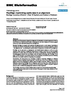
FIG. 1. Schematic picture of the three dot system. The outer dots are fixed—the left one (L) at the position −x0 and the right one (R) at x0, while the central one (C) can move (position xˆ) in a harmonic confining potential. It also interacts with a heat bath causing damping and thermal noise. The outer dots whose respective energy levels are dealigned by the device bias 共␧b兲 are coupled to the full or empty electronic reservoirs (leads), respectively. The current flows within the system due to tunneling between the left and central dot and the central and right dot and is described by the corresponding current operators IˆCL, IˆRC.

duce the numerical results with (semi-)analytic rateequation-based theory with the rates determined by the standard P共E兲 theory as functions of the model parameters. The technical details of the analytic calculations are sketched in Appendix B. We state our conclusions in Sec. V. II. THREE-DOT QUANTUM DOT ARRAY A. Model

Armour and MacKinnon16 introduced a model of a threedot array whose central dot is movable. The array is assumed to be in the strong Coulomb blockade regime in which only two charge states (none or one extra electron which we refer to as unoccupied or singly occupied) of the whole array, separated by an energy difference ␧0, are allowed in the considered bias range. This can be achieved by a suitable gating of the array which makes the two charge states energetically close while a very high charging energy prohibits addition or removal of other electrons to/from the array. The array is coupled to two leads with a high bias applied between them. The bias is smaller than the charging energy for addition or removal of other electrons but otherwise it is the largest energy scale in the model. The moving central dot interacts with its surroundings and the dissipative dynamics is described by the interaction with a generic heat bath. We modify the original model slightly in that we do not consider the additional hard wall potential at the position of the outer dots ±x0 employed by Armour and MacKinnon16 so that the central dot moves in a strictly harmonic potential in our case (see Fig. 1). While the hard wall potential is physically well motivated it complicates the numerical treatment and we believe that it does not have any significant impact on the nature of our results. Therefore, in our model the amplitude of oscillations in some regimes can exceed x0. The hard wall potential can be straightforwardly incorporated in our formalism. It should be noted, however, that the various models for dissipation used in the literature, and also adopted in our work, are best justified for the pure

205334-2

CURRENT NOISE IN A VIBRATING QUANTUM DOT ARRAY


harmonic potential. Also, as in Ref. 16, we consider spinless electrons. The Hamiltonian reads

wide-band limit. It is necessary for the so-called first Markov approximation,45,46 used later on, to hold. Further, we assume ␮L → ⬁, ␮R → −⬁. These assumptions are necessary for the derivation of the Markovian dynamics of the array. Finally, we introduce a generic heat bath consisting of an infinite set of harmonic oscillators linearly coupled to the position of the central dot (Caldeira-Leggett model47) which simulates the dissipative interaction of the center-of-mass motion of the central dot with its environment

ˆ ˆ ˆ +H ˆ ˆ ˆ ˆ =H ˆ +H H osc el el-osc + Hleads + Hel-leads + Hbath + Hosc-bath ˆ , +H CT

共1a兲

where 2 2 2 ˆ = pˆ + m␻0xˆ , H osc 2 2m

共1b兲

describes the mechanical center-of-mass motion of the central dot as a one-dimensional harmonic oscillator with mass m and frequency ␻0. The next two terms specify the electronic structure of the array in the strong Coulomb blockade regime (i.e., no double occupancy in the whole array—the vectors 兩I典 with I = 0 , L , C , R span its entire electronic Hilbert space) and the electromechanical coupling within the array ␧b ␧b ˆ ˆ +H 兩L典具L兩 − 兩R典具R兩 + ␧0兩0典具0兩 H el el-osc = 2 2 + tL共xˆ兲共兩L典具C兩 + 兩C典具L兩兲 + tR共xˆ兲共兩C典具R兩 + 兩R典具C兩兲 −

␧b xˆ兩C典具C兩 2x0

共1c兲

with tL共xˆ兲 = −V0e−␣共x0+xˆ兲, tR共xˆ兲 = −V0e␣共xˆ−x0兲. We associate the energies ␧b / 2, −␧b / 2, and ␧0 with the left and right dot and the empty array, respectively, while the energy level of the central dot is chosen as the reference energy, and hence put to zero. The device bias ␧b is the difference between the energy of the left and the right dot (which can be induced by suitable gating of the different dots) and 2x0 is the distance between the two outer dots. The terms proportional to tL,R共xˆ兲 describe a position-dependent hopping between the left and central or central and right dots enabling the tunneling current to flow through the array. These terms contribute both to the static part of the Hamiltonian (zeroth order in xˆ) as well as to the electromechanical coupling. The parameter ␣ equals the inverse tunneling length and determines the strength of the exponential xˆ dependence of the hopping elements which may lead to the shuttling instability.10,16,22 The last term gives the electromechanical coupling due to the electrostatic force acting on the oscillator when the central dot is charged. The outer dots of the array are assumed to couple via standard tunneling terms to two noninteracting leads ˆ ˆ H leads + Hel-leads =

␧k␤cˆk†␤cˆk␤ 兺 k;␤=L,R +

Vk␤共cˆk†␤兩0典具␤兩 + 兩␤典具0兩cˆk␤兲. 兺 k;␤=L,R

共1d兲

The leads are held at different electrochemical potentials ␮L,R whose difference gives the bias across the array. We assume that the tunneling densities of states ⌫␤共␧兲 = 2␲ / ប兺k兩Vk␤兩2␦共␧ − ␧k␤兲 are energy independent (and equal, just for convenience), i.e., ⌫␤共␧兲 = ⌫, known as the

ˆ ˆ ˆ H bath + Hosc-bath + HCT =

兺j −

冉

冊

m j␻2j xˆ2j pˆ2j + − 2 2m j

m 2 2 ⌬␻ xˆ . 2

兺j c jxˆ jxˆ 共1e兲

The bath is characterized by its spectral density J共␻兲 = 共␲ / 2兲兺 j共c2j / m j␻ j兲␦共␻ − ␻ j兲. We take it in the Ohmic form47 J共␻兲 = m␥␻ f共␻ / ␻c兲 where we have introduced the damping coefficient ␥ and f共␻ / ␻c兲 is a model specific cutoff function f共x → 0兲 → 1. As long as the cutoff frequency is much bigger than the frequency of the oscillator 共␻c Ⰷ ␻0兲 f would only contribute to the renormalization of ␻20 → ␻20 + ⌬␻2 with ⌬␻2 = −1 / m兺 j共c2j / m j␻2j 兲 = −2 / ␲ 兰⬁0 d␻关J共␻兲 / m␻兴 = −2␥ / ␲ 兰⬁0 d␻ f共␻ / ␻c兲. Here, we ˆ canhave explicitly included the standard counter-term H CT celing this renormalization so that the bath solely induces dissipation and the cutoff function can be replaced by unity. B. Generalized master equation

For the description of the model we use the language of quantum dissipative systems.47 As the “system” (or “device”) we take the electronic states of the dots in the array (including the unoccupied state) plus the one-dimensional oscillator describing the center-of-mass motion of the central dot. The electronic leads coupled to the outer dots and the heat bath interacting with the center-of-mass degree of freedom of the central dot constitute the reservoirs. The Hamiltonian of the ˆ +H ˆ +H ˆ ˆ =H system is then H 0 osc el el-osc. For further reference we also introduce the Hamiltonian of all mechanical degrees of freedom, i.e., of the oscillator and the bath, reading ˆ +H ˆ ˆ ˆ ˆ ⬘ =H H osc osc-bath + Hbath + HCT. The task is now to inteosc grate out the degrees of freedom of the reservoirs to end up with an equation of motion for the system density operator. We outline how the derivation proceeds in two steps first integrating out the leads in the high bias limit and then the heat bath in the weak coupling limit to get a generalized master equation (GME) for the system density operator. As in previous papers,16,22,48 we work in the high bias limit in which the bias between the leads is much higher than any other involved energy scale but the charging energy (cf. Ref. 42 and Fig. 1). The high bias assumption together with the wide-band limit means that after integrating out the leads the resulting dynamics of the system and heat bath is still Markovian. Following the derivation by Gurvitz and Prager42 one can obtain the equations of motion for the density matrices ␴ˆ 共n兲共t兲 of the system plus heat bath resolved with respect to the number of electrons n which have tunneled to the

205334-3



right lead by time t. We use the block notation analogous to the one used in Ref. 16 (ប = 1 throughout the paper except for figures) 共n兲 ˆ ⬘ , ␴ˆ 共n兲兴 − ⌫␴ˆ 共n兲 + ⌫␴ˆ 共n−1兲, n = 0,1, . . . ␴˙ˆ 00 = − i关H 00 osc 00 RR 共n兲 ˆ ˆ +H ˆ⬘ +H ˆ 共n兲兴兩J典 + 具I兩Kdriv␴ˆ 共n兲兩J典 ␴ˆ˙ IJ = − i具I兩关H el el−osc, ␴ osc

共2兲

for I,J = L,C,R.

Here ␴ˆ IJ = 具I兩␴ˆ 兩J典 are still operators in the oscillator and bath space. The “driving” kernel Kdriv due to the coupling to the leads acts nontrivially only on the electronic degrees of freedom and as unity on all the others. Hence also it can be written in the block notation Kdriv␴ˆ = ⌫

冢

␴ˆ 00 0

冣

0

− ␴ˆ LR/2

0

− ␴ˆ CR/2 ,

− ␴ˆ RL/2 − ␴ˆ RC/2

− ␴ˆ RR

共3兲

where the tunneling density of states ⌫ describes the injection rate from/to the leads. We still have to consider the off-diagonal block elements of the density matrix ␴ˆ 0I , ␴ˆ I0 with I = L , C , R. They describe coherences between system states containing a different number of electrons. In the formalism by Gurvitz and Prager42 these off-diagonal elements are identically zero by the construction of the theory (see also Ref. 16). In other works, e.g., in Ref. 46, they can in principle appear, at least indirectly. In any case, whatever method is applied to our system, they are always decoupled from the rest of the elements. Moreover, they do not enter any expressions for quantities of physical interest that we consider, and can therefore be discarded. The GME for ␴ˆ 共t兲 = 兺n␴ˆ 共n兲 is found by summing Eq. (2) over n with the boundary condition42 ␴ˆ 共−1兲 ⬅ 0. Due to this boundary condition the GME for ␴ˆ 共t兲 is formally the same as Eq. (2) just with the superscript index 共n兲 omitted. This GME is used in Sec. IV C and Appendix B in the sequential tunneling limit to derive a rate equation, from which both current and noise can be calculated, and compared to the full numerical evaluation. In general, there is no simple approximative analytic treatment of the problem nor is a direct numerical solution possible due to the presence of the infinite number of bath degrees of freedom as a part of the system. To proceed we have to integrate out the bath degrees of freedom to be left with the electronic and oscillator degrees of freedom only which can be handled numerically. This could in principle be done in the weak coupling limit between the device and the heat bath by a perturbation expansion in the c j’s. This would amount to finding the “free” evolution of the device first, i.e., the evolution without the coupling to the heat bath but with coupling to the leads included. However, this free evolution is not unitary which significantly hinders any attempt to proceed. Even in the case of small coupling ⌫ to the leads, when the driving Liouvillean is neglected,49 one should diagonalize the device Hamiltonian (including the electromechanical coupling) and use the exact eigenenergies and eigenvectors as the input into the weak coupling prescription,50,51 as was recently done in a dissipative double-dot system in Ref. 52.

Rather than following this lengthy procedure, we used the standard quantum optical damping kernel for a single harmonic oscillator in the rotating wave approximation45,53 also used in previous studies.16,20,48 Strictly speaking, this can be justified only in the case of weak electromechanical coupling and small injection. Nevertheless, we believe that the genuine nonequilibrium phenomena described later on are captured qualitatively correctly even with this kernel since the kernel mostly serves just as a “convergence factor” to stabilize the stationary solution. As will be seen below, the sequential tunneling limit is extremely well captured within the adopted approach. This is perhaps not too surprising since in that limit the coherence between different dots is negligible. On the other hand, the clear advantage of our choice of the damping kernel is that it preserves charge conservation throughout the whole circuit while this may not happen in general in the weak coupling prescription (see Sec. III D). Refinements of the present approaches to deal with the above issues are in our opinion a challenging task for the future modeling of NEMS. We would like to point out that the above-mentioned concerns about additivity of the two baths apply also to the case of the one-dot setup traditionally used for the description of the shuttling phenomena22,33,34 but the problem stemming from the coherence present within the array is absent there. Bearing all these cautions in mind, we are ready to state the generalized master equation16 for the n-resolved density matrix of the system 共n−1兲共n兲共n兲共n兲 ˆ , ␳ˆ 共n兲兴 + L ˆ 00 ␳˙ˆ 00 = − i关H − ⌫␳ˆ 00 + ⌫␳ˆ RR osc 00 damp␳ 共n兲共n兲 ˆ +H ˆ +H ˆ ˆ 共n兲兴兩J典 + Ldamp␳ˆ IJ ␳˙ˆ IJ = − i具I兩关H el osc el-osc, ␳

+ 具I兩Ldriv␳ˆ 共n兲兩J典 for I,J = L,C,R.

共4兲

The commutator terms in Eq. (4) describe the coherent evolution of the isolated device. The driving kernel Ldriv is given just by substitution ␴ˆ → ␳ˆ in Eq. (3) Ldriv␳ˆ = ⌫

冢

␳ˆ 00 0

冣

0

− ␳ˆ LR/2

0

− ␳ˆ CR/2 .

− ␳ˆ RL/2 − ␳ˆ RC/2

− ␳ˆ RR

共5兲

Finally, the damping kernel16 (acting as unity on the electronic degrees of freedom) reads

␥ Ldamp␳ˆ = − ¯n共aâˆ†␳ˆ − 2aˆ†␳ˆ aˆ + ␳ˆ aâˆ†兲 2 ␥ ¯ + 1兲共aˆ†aˆ␳ˆ − 2aˆ␳ˆ aˆ† + ␳ˆ aˆ†aˆ兲, − 共n 2

共6兲

where ␥ is the damping rate and ¯n = nB共␻0兲 = 关exp共␻0 / kBT兲 − 1兴−1 is the mean occupation number of the oscillator at temperature T. This term describes the effect of the environment on the oscillator, consisting in mechanical damping and random quantum and thermal excitation (Langevin force). The issue of the appropriate choice of the damping kernel is, however, quite subtle in many respects even in the case of a simple harmonic oscillator used here. There is a well-known

205334-4



dilemma between the rotating wave approximation form (conserving the positive definiteness of the resulting density matrix) which we use in this work versus the translationally invariant form (yielding correct equations of motion for the mean coordinate and momentum) used previously.22,34 It is known that this dilemma cannot be solved within the Markov approximation (without relaxing the condition of approach to the canonical thermal equilibrium state for asymptotic times; for a thorough discussion of this issue see Ref. 54). We have carried out a number of numerical checks, and have found out that in the present case there are only minor differences in the obtained results. A practical advantage of the present choice is that it leads to faster numerical convergence. We can recast the GME (4) into a compact form

called superoperators (or supermatrices). In the following, all superoperators will be denoted by calligraphic symbols and the vectors of the superspace in the bra-ket notation will be distinguished from the normal vectors in the Hilbert space by double brackets, e.g., Vˆ ↔ 兩v典典 with Vˆ being a “normal” quantum mechanical operator. ⬁ If 兵兩n典其n=1 is an orthonormal basis in the Hilbert space ⬁ of the system then all the projectors 兵兩m典具n兩 ⬅ 兩mn典典其m,n=1 form an orthonormal basis of the corresponding Liouville space with respect to the scalar product 具具a 兩 b典典 = Trsys共Aˆ†Bˆ兲. The matrix representation of superoperators follows analogously to the normal Hilbert space case, i.e., O = 兺kl,mn兩kl典典具具kl兩O兩mn典典具具mn兩 = 兺kl,mn兩kl典典Okl,mn具具mn兩. There is a unique mapping between matrices representing the operators in the Hilbert space and the vectors in the Liouville ˆ = 兺兩k典O 具l兩 represented by the space. The operator O k,l kl matrix Okl corresponds to the vector 兩o典典 = 兺klOkl兩kl典典 represented by the column vector o = 共O11 , O12 , O13 , . . . , O21 , O22 , O23 , . . . 兲T (the exact ordering depends on the chosen ordering of the double indices kl). Therefore, we will in the following use the two representations interchangeably.

␳˙ˆ 共n兲 = 共L − I0R兲␳ˆ 共n兲 + I0R␳ˆ 共n−1兲 , ⬁

␳˙ˆ = L␳ˆ with ␳ˆ =

兺 ␳ˆ 共n兲 and ␳ˆ 共−1兲 ⬅ 0,

共7兲

n=0

where I0R␳ˆ = ⌫兩0典具R兩␳ˆ 兩R典具0兩 (the symbol I0R denotes the superoperator of the particle current across the junction 0R between the right dot and the right lead, for a discussion on superoperators see below). The dynamics of the device described by the above generalized master equation (7) constitutes a quantum Markov process.45 The Liouvillean L determines the evolution superoperator exp共Lt兲 which fully characterizes the resulting quantum Markov process. It can be used to calculate arbitrary multitime correlation functions of any system operators, i.e., operators acting as unity on the Hilbert space of the reservoirs, by using the multitime structure of the quantum Markov process (often referred to as the quantum regression theorem)—for details see Ref. 45, Sec. 5.2 or Ref. 53, Sec. 3.2. Therefore, not only the mean value of the stationary current within the array as in Refs. 16 and 20, can be evaluated in this way, but also its higher order correlation functions, in particular the current noise spectrum, become accessible. The calculation can only be done for the junctions within the array. For the outer junctions between the outer dots and leads the quantum regression theorem cannot be applied since the corresponding current operators involve the lead electrons, thereby not being system operators. However, the n-resolved form of the GME (7) enables us to calculate the current noise spectrum also for those junctions. Both methods yield equivalent results as we will show later in Sec. III D.

III. NOISE CALCULATION A. Definition and properties of the current noise spectrum

In this subsection we define the current noise spectra for different junctions present in our model and analyze several of their properties. First, we find the current operators across different junctions. From the equations of motion for the operators of the occupation of the respective dots nˆJ = 兩J典具J兩, J = 0, L, C, R reading e

共8兲

we identify the corresponding charge current operators (electronic charge is e ⬍ 0; electrons flow from left to right) Î ⬅ Î ⬅ Î = − e d Nˆ 共t兲 0− L+ L0 L dt = ie

C. Notational details

The linear operator L which acts on the density operators, as specified by Eqs. (4)–(7), can be handled (at least formally) as any other linear operator. We can associate a matrix (infinite in our case) with it and perform standard linear algebra operations. In order to avoid confusion with “normal” quantum mechanical operators acting in the “normal” Hilbert space of the system, the vector space of “normal” operators is called the Liouville space or the superspace, and the Liouvillean and other linear operators acting in the superspace are

d ˆ 兴 = Î − Î nˆJ = − ie关nˆJ,H J+ J− dt

兺k VkL共cˆkL† 兩0典具L兩 − 兩L典具0兩cˆkL兲,

共9a兲

Î ⬅ Î ⬅ Î = iet 共xˆ兲共兩L典具C兩 − 兩C典具L兩兲, L− C+ CL L

共9b兲

Î ⬅ Î ⬅ Î = iet 共xˆ兲共兩C典具R兩 − 兩R典具C兩兲, C− R+ RC R

共9c兲

Î ⬅ Î ⬅ Î = e d Nˆ 共t兲 = ie R− 0+ 0R R dt

兺k VkR共兩R典具0兩cˆkR − cˆkR† 兩0典具R兩兲, 共9d兲

† † cˆkL , NˆR = 兺kcˆkR cˆkR being the operators of the with NˆL = 兺kcˆkL number of particles in the left and right lead, respectively. We next define different current-current correlation functions (a , b = L0, CL, RC, 0R)

205334-5



Cab共␶兲 = lim

t→⬁

冋

1 ˆ 具兵Ia共t + ␶兲,Iˆb共t兲其典 − 具Iâ共t + ␶兲典具Iˆb共t兲典 2

1 = lim 具兵⌬Iâ共t + ␶兲,⌬Iˆb共t兲其典, t→⬁ 2

册

ˆ 共t兲 = eN ˆ 共0兲 = ˆ 共t兲 − eN with Q R R R 共10兲

which in the stationary limit are functions of ␶ only. We also note the property Cab共−␶兲 = Cba共␶兲. The current noise spectrum is55

冕

⬁

d␶Cab共␶兲ei␻␶ .

共11兲

−⬁

The diagonal elements Saa共␻兲 of the noise matrix are nonnegative as can be shown by using the Lehmann representation. In general, for an arbitrary frequency the noise depends on the position where the current is measured. However, in the limit ␻ → 0 charge conservation implies that the noise becomes independent of the measurement position along the circuit, i.e., Saa共0兲 = Sbb共0兲 = Sab共0兲 = Sba共0兲, a ⫽ b and it also equals the shot noise component of the spectrum measured in the leads. This statement is proven by considering current correlation functions for two adjacent junctions J+, J−.56 The charge conservation condition (8) gives 1 1 CJ+J+共␶兲 = 具兵⌬IˆJ+共␶兲,⌬IˆJ+其典 = 具兵⌬IˆJ−共␶兲,⌬IˆJ+其典 2 2

共12兲

which implies SJ+J+共0兲 = SJ−J+共0兲. The relation Cab共−␶兲 = Cba共␶兲 yields SJ−J+共−␻兲 = SJ+J−共␻兲 and by using the charge conservation again we can finally establish SJ+J−共0兲 = SJ−J−共0兲. Altogether we find that the zerofrequency noise is the same for any combination of the junctions, i.e., Sab共0兲 = S共0兲艌 0 for any a, b (not necessarily adjacent; this generalization is straightforward). The current operators IˆCL, IˆRC Eqs. (9b) and (9c) between the dots are obviously system operators in the sense that they operate as unity on the degrees of freedom of the leads and the heat bath. Therefore, we can use the formalism of quantum Markov processes to evaluate correlation functions involving these operators using the quantum regression theorem—this will be done in Sec. III B. This is not the case for the operators of current between the outer dots and leads Î , Î given by Eqs. (9a) and (9d). However, the noise L0 0R spectra across these two junctions can still be calculated using the n-resolved form of the GME (7) with the help of the following identity for the zero-frequency current noise (for the junction 0R, the case L0 is analogous): d ˆ2 兩共具QR共t兲典 − 具QˆR共t兲典2兲兩t→⬁ = dt

冕

⬁

−⬁

共13兲

This identity suggests the interpretation of the zerofrequency current noise as the “charge diffusion coefficient”57 and will be used in Sec. III C for an alternative evaluation of the zero-frequency current noise. The equivalence of the two approaches is shown explicitly in Sec. III D. We finally comment on the physical relevance of the noise spectra calculated in this paper. Since the zero-frequency noise is position independent the noise calculated for the junctions within the system should also be measured in the leads. However, in practice there is always the important 1 / f contribution to the noise which actually dominates experiments for very low frequencies and which is not accounted for in our model. Therefore, as mentioned in Ref. 58, the measurements of the shot noise must be performed at nonzero frequencies of the order of 1 kHz where the 1 / f noise component becomes insignificant. However, the shot noise measured in this way is still appropriately described by the zero-frequency current noise calculations since its typical frequency scale is of the order of 1 THz. B. Quantum regression theorem (QRT)

With QRT it is possible to calculate the current noise within the system (i.e., for ÎCL, ÎRC). For ␶ 艌 0 QRT gives (cf. Ref. 45, Sec. 5.2) 1 Cab共␶兲 = Trsys共Iâ exp共L␶兲兵Iˆb, ␳ˆ stat其兲 − I2 2

1 d 具兵e⌬nˆJ共␶兲,⌬IˆJ+其典 + 2 d␶ 1 d 具兵e⌬nˆJ共␶兲,⌬IˆJ+其典 = CJ−J+共␶兲 + 2 d␶

dt⬘Î0R共t⬘兲.

0

with ⌬Iâ共t兲 = Îa共t兲 − 具Iâ共t兲典,

Sab共␻兲 =

冕

t

d␶C0R,0R共␶兲 = S0R,0R共0兲

共14兲

for a , b = CL , RC, where I = limt→⬁具Iâ共t兲典 = Trsys共Iâ␳ˆ stat兲 is the stationary current (constant throughout the circuit). In case ␶ ⬍ 0 we use the symmetry property Cab共−␶兲 = Cba共␶兲. Now, let us evaluate the spectrum Sab共␻兲 =

冕冕

⬁

d␶Cab共␶兲ei␻␶

−⬁

=

⬁

0

d␶Cab共␶兲ei␻␶ +

冕

⬁

d␶Cba共␶兲e−i␻␶ .

共15兲

0

+ 共␻兲, the secWe consider in detail the first term denoted Sab − ond one 关Sba共␻兲兴 follows analogously. Introducing a convergence factor ␻ → ␻ + i0 we get

1 1 + Sab 共␻兲 = Trsys共Iâ共− i␻ − L兲−1兵Iˆb, ␳ˆ stat其兲 + I2 . 2 i␻

共16兲

Since we are interested in the limit ␻ → 0 in the end we have to handle somehow the singularities associated with the resolvent G共−i␻兲 = 共−i␻ − L兲−1 and the second term in Eq. (16) in that limit. The problem with the inverse of L is the existence of the unique null vector 兩0典典 which is proportional to the stationary density matrix because L␳ˆ stat = 0. There exists a corresponding left eigenvector be˜兩 which is longing to the zero eigenvalue of L denoted by 具具0 ˜ not just the Hermitian conjugate of 兩0典典 (i.e., 具具0兩 ⫽ 兩0典典†) be-

205334-6



cause L is non-Hermitian. However, since Trsys共LAˆ兲 = 0 for ˜兩 ↔ 1ˆ , i.e., any system operator Aˆ we deduce that 具具0 ˆ ˆ ˜ 具具0兩L兩a典典 ⬅ Trsys共1LA兲 = 0. ˜兩 ↔ 1ˆ with 具具0 ˜ 兩 0典典 = 1 allowThus, we have 兩0典典 ↔ ␳ˆ stat, 具具0 2 ˜ ing us to define the projectors P = P = 兩0典典具具0兩, Q = 1 − P. Using these projectors and the relations PL = LP = 0, L = QLQ the resolvent can be expressed as

ˆ 共t兲典 = e兺 nP 共t兲, right lead by time t given by 具Q R n n 2 2 2 ˆ 共t兲典 = e 兺 n P 共t兲. Using the definition of the current (9d) 具Q n n R and the identity (13) we find the stationary mean current and the zero-frequency current noise43

冏

I0R = e

S0R,0R共0兲 = e2

1 1 1 Q ⬇ − P − QL−1Q =− P−Q i␻ i␻ i␻ + L 共17兲

t→⬁

n2 Pn共t兲 −

n

冉兺

nPn共t兲

n

n Pn共t兲 − 2

nPn共t兲

n

nP˙n共t兲

冊

冊册冏 2

t→⬁

共22兲

.

n

1 = − I2 , i␻

共21兲

, t→⬁

t→⬁

We evaluate P˙n共t兲 from Eq. (7) and find P˙n共t兲 = Trsys关I0R共␳ˆ 共n−1兲共t兲 − ␳ˆ 共n兲共t兲兲兴

共23兲

and consequently

1 Trsys共Iâ␳ˆ stat兲Trsys共兵Iˆb, ␳ˆ stat其兲 2i␻ 共18兲

which cancels the last term of Eq. (16). Applying the same − 共0兲 we find procedure to Sba + − 共0兲 + Sba 共0兲 Sab共0兲 = Sab

If we introduce the superoperators of (particle) current ICL, IRC defined by their action on the system density matrix as follows eIa␳ˆ = 21 兵Iâ , ␳ˆ 其, a = CL , RC with the property ˜ 兩I 兩0典典 we can rewrite the above equaI = eTrsysIa␳ˆ stat = e具具0 a tion in a compact form

兺n P˙n共t兲 = 0,

共24兲

兺n nP˙n共t兲 = Trsys冉I0R兺n ␳ˆ 共n兲共t兲冊 = Trsys关I0R␳ˆ 共t兲兴,

共25兲

冋冉兺

共26兲

兺n n2P˙n共t兲 = Trsys

1 = − 关Trsys共IâR兵Iˆb, ␳ˆ stat其 + ÎbR兵Iâ, ␳ˆ stat其兲兴. 共19兲 2

˜ 兩I RI + I RI 兩0典典 Sab共0兲 = − e2具具0 a b b a

n

2˙

2

⫻

1 ˜兩兵Iˆ , ␳ˆ stat其兲 Trsys共Iâ兩0典典具具0 b 2i␻ =−

nP˙n共t兲

= e

n

where we have defined the pseudoinverse of the Liouvillean R ⬅ QL−1Q. Substituting the term −iP / ␻ in the first term of Eq. (16) gives −

d dt

冏冏兺冏

冏冋兺冉兺冉兺冊册冏

= e

1 P − R for small ␻ , i␻

兺n nPn共t兲

冏冋兺

G共− i␻兲 = 共− i␻ − L兲−1 = 共− i␻P − i␻Q − QLQ兲−1

=−

d dt

I0R 2

n␳ˆ 共n兲共t兲 + ␳ˆ 共t兲

n

冊册

,

where according to the definition 兺n␳ˆ 共n兲共t兲 = ␳ˆ 共t兲. Now, we employ an operator-valued generalization of the standard generating function technique to calculate 兺nn␳ˆ 共n兲共t兲. We introduce the object Fˆ共t ; z兲 = 兺n␳ˆ 共n兲共t兲zn which has the properties Fˆ共t ; 1兲 = ␳ˆ 共t兲, 兩⳵Fˆ共t ; z兲 / ⳵z兩z=1 = 兺nn␳ˆ 共n兲共t兲 and satisfies the equation of motion

a,b = CL,RC.

⳵ˆ F共t;z兲 = 关L + 共z − 1兲I0R兴Fˆ共t;z兲. ⳵t

共20兲 This equation constitutes the main formal result of this subsection and forms the basis for further formal manipulations and eventually the numerical treatment. C. Counting variable approach—evaluation of the charge diffusion coefficient

Using the generating function the current noise formula (22) can be rewritten as

冏冉再冋冏

S0R,0R共0兲 = e2 Trsys I0R 2

Using the n-resolved form of the GME (7) we could in principle find the full counting statistics (FCS) of the charge transfer through the junction between the right dot and the right lead, i.e., the probabilities Pn共t兲 that n electrons tunneled into the right lead across the junction by time t given by Pn共t兲 = Trsys␳ˆ 共n兲共t兲. Here, we are only interested in the evaluation of the zero-frequency noise for which we just need the mean and the mean square charge tunneled into the

共27兲

冏册冎冋冏冏册冊冏

⳵ ˆ F共t;z兲 ⳵z

+ Fˆ共t;1兲

z=1

⳵ ˆ F共t;z兲 − 2Trsys关I0RFˆ共t;1兲兴Trsys ⳵z

z=1

. t→⬁

共28兲 The equation of motion for Fˆ共t ; z兲 (27) can be solved via the ˜ Laplace transform Fˆ共s ; z兲 = 兰⬁dte−stFˆ共t ; z兲 giving

205334-7

0



˜ 关s − L − 共z − 1兲I0R兴Fˆ共s;z兲 =

兺n ␳ˆ 共n兲共0兲zn ,

共29兲

pression as expected and necessary. Similarly, for the L0 junction one finds SL0,L0共0兲 = eI − 2e2Trsys共IL0RIL0␳ˆ stat兲

with ␳ˆ 共n兲共0兲 being the initial conditions. Recalling the definition of the resolvent G共s兲 = 共s − L兲−1 of the Liouvillean we arrive at ˜ˆ F共s;1兲 = G共s兲␳ˆ 共0兲

冏

⳵ ˜ˆ F共s;z兲 ⳵z

冏

共30兲

= G共s兲I0RG共s兲␳ˆ 共0兲 + G共s兲 z=1

兺n n␳ˆ 共n兲共0兲.

Because the large-t behavior of Fˆ共t ; z兲 is related to the small˜ s behavior of Fˆ共s ; z兲 we study the asymptotics of the above

expressions as s → 0+. This is entirely determined by the resolvent G共s兲 in the small-s limit. We can use the results from the previous subsection and substitute −i␻ → s to get the leading asymptotics of G共s兲 for s → 0+. Thus, we obtain P 1 ˜ˆ F共s;1兲 ⬇ ␳ˆ 共0兲 = ␳ˆ stat s s

⳵ ˆ F共s;z兲 ⳵z

冏

⬇ z=1

冋

共32兲

1 1 PI0RP␳ˆ 共0兲 − PI0RR␳ˆ 共0兲 s2 s + RI0RP␳ˆ 共0兲 − P

兺n n␳ˆ 共n兲共0兲

兩Fˆ共t;1兲兩t→⬁ ⬇ ␳ˆ stat

⳵ ˆ F共t;z兲 ⳵z

with IL0␳ˆ = ⌫兩L典具0兩␳ˆ 兩0典具L兩.

册

冏

冉

⬇ ␳ˆ stat z=1,t→⬁

. 共33兲

共34兲

冊

I t + Cinit − RI0R␳ˆ stat , 共35兲 e

where Cinit = Trsys关兺nn␳ˆ 共n兲共0兲 − I0RR␳ˆ 共0兲兴 is an initial conditions dependent constant and the stationary current is given by I = e Trsys共I0R␳ˆ stat兲. The corrections to the large time asymptotic behavior are exponentially small—the approach to the stationary state in a Markovian system is exponential. In particular, it is important that there is no 1 / t correction to 兩Fˆ共t ; 1兲兩t→⬁ (which would correspond to a ln s-like divergence in the resolvent as s → 0+) since it would combine with the linearly in t divergent term in ⳵ / ⳵z兩Fˆ共t ; z兲兩z=1,t→⬁ to yield a finite term in Eq. (28). We substitute the above asymptotic formulas into Eq. (28), use the definition of the stationary current and the identities Trsys ␳ˆ stat = 1, Trsys R · = 0 to get the final result for the zero-frequency current noise at the 0R junction, S0R,0R共0兲 = eI − 2e2Trsys共I0RRI0R␳ˆ stat兲 ˜ 兩I − 2I RI 兩0典典. = e2具具0 0R 0R 0R

We show the equality between the expressions (20), (36), and (37). Both formulas contain the same basic building block consisting of terms of the type IaRIb. However, there is an obvious difference: The presence of the so-called selfcorrelation or Schottky term (proportional to the mean current) in formulas (36) and (37). Yet, they give the same value for the zero-frequency noise in the end as we now proceed to show. The independence of the zero-frequency noise from the position along the circuit has been shown quite generally in Sec. III A using the charge conservation. Thus, the only task now is to find the corresponding expression for the charge conservation within the superoperator language. Following the purely stochastic analogy59 we find that the charge conservation condition (8) is expressed in terms of superoperators by the following equation: 关NJ,L兴 = IJ+ − IJ−

In the time domain this gives

冏

共37兲

D. Equivalence of different approaches

共31兲

冏

˜ 兩I − 2I RI 兩0典典 = e2具具0 L0 L0 L0

with the superoperators of occupation of the “site” J, J = 0, L, C, R being given by NJ␳ˆ = 21 兵兩J典具J兩 , ␳ˆ 其, the current superoperators Ia were defined previously and the convention for J± is the same as in Eqs. (9). The above relation follows from the definitions of the respective quantities and Eqs. (4)–(8). Since the heat bath does not couple directly to the electronic degrees of freedom its degrees of freedom do not enter explicitly the current and occupation operators, cf. Eqs. (8) and (9), and are therefore absent from the corresponding superoperators. We believe that this property should be reflected in the identity 关NJ , Ldamp兴 = 0 for any choice of the damping kernel. Obviously, this condition is fulfilled for our choice of the damping kernel (6). However, for the generic weak coupling prescription50,51 for the damping kernel the above identity may not be satisfied which would break the charge conservation.60 This raises the possibility that there is another problem with the Markovian weak damping prescription analogous to the translational invariance issue threatening the charge conservation for damped NEMS involving coherent charge transfer (such as our quantum dot array). This issue deserves further investigation. The charge conservation relation (38) is used to prove the ˜ 兩I 兩0典典 and position independence of the mean current I = e具具0 a the zero-frequency noise Sab共0兲 for any a, b. The mean current conservation follows from ˜ 兩I 兩0典典 I = e具具0 J+

共36兲

In the algebra leading to Eq. (36) the linearly divergent terms in t and the initial condition terms cancel identically so that we are left with a regular, initial-condition-independent ex-

共38兲

˜ 兩I 兩0典典 + e具具0 ˜ 兩关N ,L兴兩0典典 = e具具0 ˜ 兩I 兩0典典 = e具具0 J− J J−

共39兲

˜ 兩L = 0. Analogously, we prove the equivadue to L兩0典典 = 0 , 具具0

205334-8



lence, for example, between S0R,0R共0兲 Eq. (36) and SRC,RC共0兲 Eq. (20). Substituting Eq. (38) for J = R into the expression (20) for SRC,RC共0兲 we get in the first step

auxiliary quantities ⌺ˆ a = eRIa␳ˆ stat determined by the equation

˜ 兩I RI 兩0典典 = e2具具0 ˜ 兩关I ,N 兴兩0典典 SRC,RC共0兲 = − 2e2具具0 RC RC RC R ˜ 兩I RI + I RI 兩0典典 − e2具具0 0R RC RC 0R ˜ 兩I RI + I RI 兩0典典 = − e2具具0 0R RC RC 0R ⬅ SRC,0R共0兲 = S0R,RC共0兲

共40兲

˜兩 and finding bearing in mind LR = RL = Q = 1 − 兩0典典具具0 1 ˆ e关IRC , NR兴␳ˆ = 4 关关IRC , 兩R典具R兩兴 , ␳ˆ 兴 which yields zero when traced over. We proceed similarly in the second step and obtain ˜ 兩I RI 兩0典典 + e2具具0 ˜ 兩关I ,N 兴兩0典典. S0R,0R共0兲 = − 2e2具具0 0R 0R 0R R 共41兲 The second term can be evaluated as 关I0R , NR兴 = 关N0 , I0R兴 = I0R recovering finally the expression (36) for S0R,0R共0兲. By extending the argument to other combinations of the junctions we can summarize the formulas for the zerofrequency noise S共0兲 = SI+,J+共0兲 for any I, J = 0, L, C, R in the compact form as [compare with the analogous expression for the purely stochastic case in Ref. 59, Eq. (26)] ˜ 兩I RI + I RI 兩0典典 S共0兲 = − e2具具0 I+ J+ J+ I+ ˜ 兩关N ,I 兴兩0典典 for any I,J. + ␦IJe2具具0 I J+

共42兲

This equation merges the two approaches into a single picture unifying both the pure quantum mechanical and pure classical stochastic formalisms. It has a quantummechanical-like form of a “mean value” of the pseudoinverse of the Liouvillean symmetrically flanked by two current superoperators corrected with the classical-like self-correlation term. The self-correlation term is only effective for the diagonal elements of the current-current correlation matrix and, moreover, is nonzero just for the outer junctions where it contributes by the mean current. E. Notes on numerical evaluation

From the results obtained thus far we see that the evaluation of the noise involves two steps. At the first step we find the stationary state ␳ˆ stat = limt→⬁ exp共Lt兲␳ˆ 0 independent of the initial condition ␳ˆ 0 and equivalently given by the equation L␳ˆ stat = 0, Trsys ␳ˆ stat = 1.

共43兲

Having found ␳ˆ stat we can fully characterize all one-time quantities pertaining to the system such as occupations of the different dots, mean current, Wigner functions of the oscillator in different charge states, etc. To evaluate the noise (second step) we have to find the pseudoinverse of the Liouvillean R = QL−1Q. In practice, we actually do not have to evaluate the whole pseudoinverse but we fix a given combination of junctions and evaluate the

ˆ = eI ␳ˆ stat − I␳ˆ stat, Tr ⌺ˆ = 0. L⌺ a a sys a

共44兲

Equation (44) has a solution since the right-hand side lies in the range of L (the trace of the right-hand side is zero) and the freedom of adding any multiple of the null vector to a particular solution is fixed uniquely by the trace condition Trsys ⌺a = 0. Of course, this is equivalent to the uniqueness and regularity of the stand-alone pseudoinverse R. Moreover, R preserves hermiticity so that the quantities ⌺ˆ a are Hermitian as they should be to give a real zero-frequency noise. This follows from the property 共LAˆ兲† = LAˆ for any Hermitian Aˆ and the trace-fixing condition Trsys⌺ˆ a = 0 of Eq. (44). Equations (43) and (44) form the starting point for the numerical implementation of the noise calculation. After the truncation of the oscillator Hilbert space to the N lowest energy states the size of the supermatrix L becomes61 10N2 ⫻ 10N2 which makes direct calculations prohibitive due to memory and computation time requirements for any realistic N of the order of 30-40. These problems with the numerical implementation of the superoperator techniques can be circumvented by employing iterative methods in which only the procedure/routine yielding LAˆ for a given Aˆ is needed.62 Obviously, this does not require the storage of the whole supermatrix L. On the other hand, as with any iterative method, the convergence of the iteration becomes an issue. In Appendix A we give a brief review of the usage of the Arnoldi iteration in our calculations. Its intent is to guide the reader through the algorithm so that it can be reproduced with the help of the mathematical references.63,64 IV. RESULTS

We now turn to the numerical results for the mean current I, zero-frequency noise S共0兲 = Sab共0兲 (for any a , b—see above), and the Fano factor F = S共0兲 / eI as functions of the device bias ␧b for different sets of the other parameters. First we present a generic plot in the parameter regime considered by Armour and MacKinnon16 and comment on the general features which we can observe in it. We then give a tentative interpretation of those features supported by phenomenological arguments and results found in different limiting cases studied further on. In particular, we consider two specific limiting cases where at least a partial comparison with approximate analytic theories can be made, namely, (i) the limit of small damping which is relevant for the issue of shuttling and strong inelastic cotunneling and (ii) the limit of weak interdot coupling which implies in a certain device bias range the sequential tunneling regime. A. Generic case

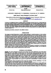
In Fig. 2 we plot the mean current, zero-frequency noise, and the Fano factor as functions of the device bias and temperature for one of the parameter sets considered in Ref. 16. We include nonzero temperature and extend the device bias

205334-9



FIG. 2. (Color online) The mean current I, zero-frequency noise S共0兲, and the Fano factor F as functions of the device bias ␧b for the static three dot array (dotted line) and the vibrating array at different temperatures given by the mean oscillator occupation number ¯n. The other parameters are V0 = 0.5ប␻0, ␣ = 0.2冑2冑m␻0 / ប, x0 = 共5 / 冑2兲冑ប / m␻0, ␥ = 0.025␻0, ⌫ = 0.05␻0 which corresponds to the case studied in Ref. 16, Fig. 6.

range considered previously16 to negative values which is relevant for nonzero temperature. The dotted lines show the results for the static array. By applying the theory of Sec. III to the static array we found analytic expressions for both the mean current and the Fano factor which we, however, do not present explicitly here since the formulas are quite involved. The mean current has a resonant peak65 around ␧b = 0 while there is a dip in the noise around ␧b = 0 which was also found analytically for a two dot array by Elattari and Gurvitz.43 They attributed the dip to the strong Coulomb interaction on the array. Our Fano factor shows a crossover from the sub-Poissonian 共F ⬍ 1兲 dip around ␧b = 0 to super-Poissonian 共F ⬎ 1兲 “shoulders” starting around ␧b ⬇ ± V0e−␣x0 which approach the Poissonian limit F = 1 for large device bias. The Poissonian limit of the Fano factor for large ␧b is understood when one notices that the current in that limit is very small. Therefore, electrons tunnel through the array sparsely and, consequently, there is no correlation between successive tunneling events which form a classical Poisson process with the (Poissonian) value of the Fano factor F = 1. While the dip around zero and the Poissonian limit for large device bias were observed in the two-dot case as well43 the Fano factor exceeding one was not present there. We attribute the super-Poissonian behavior to the (elastic) cotunneling through the central dot. Now, let us discuss the results for movable arrays. The characteristic features are the peaks in current and noise at the device bias around a nonzero integer multiple of the oscillator frequency due to electromechanical resonances. The current peaks at zero temperature (therefore, only for positive multiples of the frequency) were already observed in previous works.16,20 Some of the noise peaks have further fine structure which is even amplified in the Fano factor exhibiting a rather complex behavior around the peaks, especially at low temperature, and showing also strong temperature dependence.

The zero device bias behavior is clearly governed by the static array physics which is due to partial decoupling of the electronic and oscillator degrees of freedom at ␧b = 0 when the electrostatic interaction on the central site −共␧b / 2x0兲xˆ兩C典具C兩 is turned off. The remaining interaction stemming from the xˆ dependence of the hopping amplitudes tL共xˆ兲, tR共xˆ兲 is too weak to modify the static result in the vicinity of ␧b = 0 even for high temperatures. Some discrepancy between the static and high temperature dynamic cases around ␧b = 0 is found for higher values of ␣ ⬇ 1 (strictly quantum case from the oscillator point of view which was previously studied in the one-dot shuttling setup22,34), yet the effect is not very pronounced anyway (not shown). The peaks at nonzero multiples of the oscillator frequency were already previously attributed to electromechanical resonances.16,20 Yet, this explanation is rather broad and covers a range of processes which can be responsible for the electronic transport such as cotunneling, phonon-assisted tunneling, or shuttling occurring around different resonance peaks.16,48 The discrimination between the different processes is quite complicated since it cannot be inferred directly from a single I versus ␧b curve. Either one has to study the dependence of the curves on different parameters16 or some other kind of information about the system must be obtained. A powerful choice is to calculate and analyze the Wigner distribution functions of the oscillator in the phase space (possibly charge-resolved).20,22,48 These characterize the state of the system very well and we will use them in this study too. However, even though they are an excellent theoretical tool to study NEMS their connection to data extractable from a real NEMS experiment is at best remote. Therefore, diagnostics based on the measurement of the current statistics is clearly preferable and, therefore, our aim is to correlate particular features observed in the noise with specific transport mechanisms within the array as identified by the theoretical analysis involving also phase space plots. To achieve this goal we will study different limiting cases in which particular features of the noise (more precisely of the Fano factor) are pronounced so that they can be attributed to specific transport mechanisms. Yet, the results do not allow us to associate a given value of the Fano factor to a specific mechanism. It is more reading of the whole I versus ␧b curve at least locally around a peak which gives us the notion of what mechanism(s) are involved in the transport at that given peak. As a rule of thumb we can say that the super-Poissonian peaks of the Fano factor correspond to cotunneling through the central dot. This statement is supported by the limiting studies discussed below, and also by the following evidence from Fig. 2. The peaks only occur for small temperature and disappear with its increase pointing out to a coherent effect. They also appear predominantly at odd multiples of the oscillator frequency which is consistent with the cotunneling picture between the outer dots excluding the central one due to the energy mismatch. On the other hand, the dips in the Fano factor curves are due to some form of the sequential tunneling via the central dot. The most important aspect is that the process proceeds via a real intermediate state on the central dot in contrast to the virtual nature of the cotunneling process. The real sequential process is subject to the charge

205334-10



conservation which is a strict law strongly suppressing the Fano factor44 and causing the dip. The sequential tunneling picture still involves different mechanisms distinguished by the detailed state of the oscillator. The oscillator might be in a general nonequilibrium state during the tunneling events (this scenario encompasses both the shuttling48 and a general nonequilibrium oscillator-assisted tunneling25 mechanisms) or it could equilibrate between consecutive tunneling events. The latter case is studied in detail in Sec. IV C. The two charge transfer mechanisms (cotunneling and sequential tunneling) may coexist, i.e., part of the current is carried by the cotunneling mechanism and the other part by the sequential tunneling, and their relative weights depend strongly on the parameters. For example, the transport around ␧b ⬇ 2ប␻0 is typically governed by shuttling which results in the dip while cotunneling is dominant around ␧b ⬇ 3ប␻0 giving a peak. However, the dip around ␧b ⬇ ប␻0 in Fig. 2 changes into a clear peak when ␣ is enlarged up to ␣ ⬇ 0.4 (not shown). This behavior is still not well understood. Even more complicated is the behavior around ␧b ⬇ 4ប␻0 where there is a dip in the peak. As we show in the next subsection this corresponds to a fast crossover between the cotunneling and shuttling transport mechanisms in the vicinity of ␧b ⬇ 4ប␻0. In order to support the above statements for the generic parameters we study particular limiting cases which enable us to associate specific features of the Fano factor curves to specific mechanisms. B. Small damping: shuttling and strong inelastic cotunneling

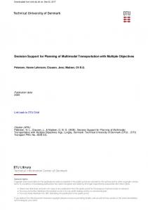
In this section results for small damping case, i.e., ␥ ⱗ I / e with I a representative value of the current (given, e.g., by its value at the zero device bias peak), are presented.66 First, we focus on the device bias range ␧b ⬇ 0 − 2.5ប␻0 where electromechanical instabilities which can be related to shuttling were inferred indirectly from the behavior of the mean current,16 predicted by quasiclassical studies,67 and subsequently directly observed in the phase space.48 The intuition and simple theoretical estimates [the zero-frequency noise is given by the ratio of the variance and the square mean of the waiting time between consecutive loading events of the classical shuttle, see Eq. (4.48) in Ref. 58] suggest that shuttling is a low noise phenomenon with the Fano factor close to zero in the nearly perfectly developed shuttling regime. This was recently confirmed by more sophisticated calculations for the classical driven28 and quantum34 shuttle in the one-dot setup. In the present, more complicated setup the shuttling is obscured by competing mechanisms (coherence between dots, strong Coulomb blockade affecting the whole array) and we will study the consequence of this fact on the behavior of the Fano factor. In Fig. 3 we show the results for the mean current and the Fano factor for zero temperature and three different (small) values of the damping. In Ref. 48 we presented the phase space plots of the oscillator which we introduce here in more detail later on [see Eq. (45) and Fig. 5]. They described a similar parameter range and showed gradually developing shuttling around ␧b ⬇ ប␻0, 2ប␻0 with increasing injection

FIG. 3. (Color online) The mean current and Fano factor for V0 = 0.76ប␻0, ␣ = 0.28冑m␻0 / ប, x0 = 5冑ប / m␻0, ⌫ = 0.2␻0, T = 0 and different values of the damping coefficient (in units of ␻0) corresponding to shuttling around ␧b ⬇ ប␻0, 2ប␻0.

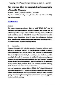
rate ⌫. At these resonance points the current has peaks moderately changing with the increase of the damping and the Fano factor has local minima with possible shoulderlike structure further from the resonance points in case of the smallest damping. As established more explicitly below, the shoulders are a signature of coherent processes through the whole array (cotunneling) and, therefore, are destroyed by the increased damping. At the same time the absolute values of the local minima of the Fano factor at the resonances become deeper by the increased damping. We conjecture that this somewhat surprising behavior can also be attributed to the destruction of the quantum coherence and to the crossover into the nonequilibrium sequential tunneling regime partially encompassing shuttling. The minimum of the Fano factor curve starts to increase again with a further increase of damping (not shown) as expected from the classical shuttling theory. The minimal value of the Fano factor achieved for the given set of parameters was Fmin ⬇ 0.25 which corresponds to a partially developed shuttling regime and was also confirmed by the phase space pictures (not shown). Next, we focus on the range ␧b ⬇ 2.5ប␻0 − 4.5ប␻0 involving two current peaks around ␧b ⬇ 3ប␻0, 4ប␻0. As we already mentioned in the generic case the peak around ␧b ⬇ 3ប␻0 corresponds to cotunneling while the behavior around ␧b ⬇ 4ប␻0 is given by a complicated interplay between both mechanisms (cotunneling and sequential tunneling). With lower damping the differences in the Fano factors of the two mechanisms become more pronounced as we show in Figs. 4 and 5. In Fig. 4 the mean current and the Fano factor as functions of the device bias ␧b are depicted for several (small) values of the damping. We see the strong damping dependence of the mean current and the Fano factor around ␧b ⬇ 3ប␻0 and in the “shoulder region” around ␧b ⬇ 4ប␻0. On the other hand the mean current as well as the Fano factor do not depend strongly on the damping in the close vicinity of ␧b ⬇ 4ប␻0.

205334-11



FIG. 4. (Color online) The mean current and Fano factor for V0 = 0.76ប␻0, ␣ = 0.28冑m␻0 / ប, x0 = 5冑ប / m␻0, ⌫ = 0.2␻0, T = 0 and different values of the damping coefficient (in units of ␻0) in the strong inelastic cotunneling/shuttling regime. The dots on the curves corresponding to ␥ = 0.0125 denote the points for which the Wigner functions in Fig. 5 are plotted.

We attribute the first type of behavior to cotunneling. It is manifested by a strong damping dependence of the current and the Fano factor, the Fano factor reaches very high values of the order of F ⬇ 50 for small enough damping. The threshold for the quasi-divergent behavior of the Fano factor is roughly ␥thresh ⬇ I / e; for the damping below this threshold the Fano factor starts to increase. We want to point out that a

WUU共X, P兲 =

冕

⬁

−⬁

giant (divergent) super-Poissonian noise was theoretically predicted for a quantum dot system in the (strong inelastic) cotunneling regime analogous to ours by Sukhorukov et al.44 The divergence of the current noise is explained as a slow switching between two or more current channels carrying different currents. We expect that the different current channels are formed from different resonant quantum states connecting the left and right dots in the cotunneling regime. Due to the small damping rate the switching between those channels is slow giving rise to the highly super-Poissonian noise. We also observed a quasidivergent Fano factor (up to F ⬇ 600) around the shuttling instability transition point in the quasiclassical limit of the original one-dot shuttle setup.34 The explanation of the divergence is again the same, i.e., the slow switching between different current channels. Contrary to the present case the two channels of the one-dot setup are both given by real sequential tunneling processes via the dot differing just by the state of the oscillator (equilibrated vs shuttling). The switching rate between the channels can be calculated semianalytically thus quantitatively confirming the proposed mechanism.68 In the three-dot case the semianalytic theory would be much more complicated and we do not attempt it. A similar mechanism for the quasidivergent Fano factor in a single-electron-transistor NEMS was also proposed recently by Blanter et al.35 Further insight to the details of the microscopic transport mechanism can be gained by studying the Wigner functions which describe the oscillator phase space quasiprobability distributions. We define Wigner functions of the unoccupied 共WUU兲, occupied 共WCC兲 central dot and their sum 共Wtot兲, respectively,

dy iPy stat stat stat e 具X − 共y/2兲兩共␳ˆ 00 + ␳ˆ LL + ␳ˆ RR 兲兩X + 共y/2兲典, 2␲

WCC共X, P兲 =

冕

⬁

−⬁

dy iPy stat e 具X − 共y/2兲兩␳ˆ CC 兩X + 共y/2兲典, 2␲

Wtot共X, P兲 = WCC共X, P兲 + WUU共X, P兲.

The behavior in the close vicinity of ␧b ⬇ 4ប␻0 characterized by a weak damping dependence of the mean current and the Fano factor (of the order of 1) seen in Fig. 4 is characteristic of shuttling. It is confirmed directly by the phase space plots in Fig. 5 where the crossover from the predominantly shuttling transport at ␧b = 3.96ប␻0 to the cotunneling regime at ␧b = 4.12ប␻0 is shown. The shuttling is evidenced by the asymmetric Wigner distributions of the occupied or empty central dot WCC, WUU, respectively (first column). The cotunneling manifests itself by the striking absence of any occupation of the central dot (last column) which proves the virtual nature of the transport in that case.

共45兲

C. Weak interdot coupling: sequential tunneling assisted by equilibrated oscillator

Here we examine the behavior of the system in the weak tunneling regime, i.e., when the hopping elements tL共xˆ兲, tR共xˆ兲 coupling the adjacent dots in the array are small and the time scale between tunneling events is correspondingly the largest in the problem. In this limit the phonon subsystem gets equilibrated between the consecutive tunneling events and the distribution of the oscillator and bath may be taken at equilibrium corresponding to the appropriate electronic state. We can then solve the GME (2) using perturbation theory keeping only the lowest order terms in the bare hopping

205334-12



FIG. 6. The four states 0 (device empty), L (left dot occupied), C (central dot occupied), R (right dot occupied) and the transition rates as described by the Markov process given by the transition matrix (46).

the results are given in Appendix B, Eqs. (B12), (B13), and (B18). The stationary state pstat satisfying Mpstat = 0 is found to be FIG. 5. (Color online) Phase space representation of the oscillator around the transition from the shuttling to the strong inelastic cotunneling regime at ␧b / ប␻0 = 3.96, 4.04, 4.12, respectively (columns from the left to the right). The respective rows show the Wigner distribution functions for the empty 共WUU兲 or occupied 共WCC兲 central dot, and the sum of the two 共Wtot = WUU + WCC兲 in the oscillator phase space (horizontal axis—coordinate in units of 冑ប / m␻0, vertical axis—momentum in 冑បm␻0, the grid is at 2.5 in the dimensionless units). The other parameters are: V0 = 0.76ប␻0, ␣ = 0.28冑m␻0 / ប, x0 = 5冑ប / m␻0, ␥ = 0.0125␻0, ⌫ = 0.2␻0, T = 0. The parameters correspond to the dots in Fig. 4. The Wigner functions are normalized within each column.

parameter V0 which turns out to be equivalent to the P共E兲 theory.69 The coherence of the electron transfer process from the left to the right dot is broken during the transfer by the long enough interaction with the phonon subsystem acting as equilibrated thermal bath and, therefore, the resulting picture is just sequential tunneling (ST) via the central dot, at least in the device bias range where the above assumptions hold. We defer a more detailed discussion until the end of this subsection where the assumptions will be reexamined and their validity clarified in view of the obtained results. When we carry out the approximate solution of Eq. (2) in the lowest order in V0 as described in Appendix B we obtain the rate equation (B6) describing a classical Markov process of the sequential electron transfer between the 4 states which is depicted in Fig. 6. After introducing the vector of occupation probabilities p = 关P0 , PL , PC , PR兴T the equation can be rewritten in the matrix form p˙ = Mp with the transition matrix

M=

冢

−⌫

0

0

⌫

⌫

− ⌫CL

⌫LC

0

0

⌫CL

− 共⌫LC + ⌫RC兲

⌫CR

0

0

⌫RC

− 共⌫CR + ⌫兲

冣

pstat = N

冢

⌫CL⌫RC ⌫RC⌫ + ⌫LC共⌫CR + ⌫兲 ⌫CL共⌫CR + ⌫兲 ⌫CL⌫RC

冣

共47兲

with the normalization constant N = 关⌫RC⌫ + ⌫LC共⌫CR + ⌫兲 + ⌫CL共⌫CR + 2⌫RC + ⌫兲兴−1. To calculate the mean current and, in particular, the current noise one can proceed following two possible equivalent ways which parallel in close analogy the two methods used in Secs. III B and III C. In the first method found in Refs. 58, 59, and 70 one defines an effective operator for the current running between, e.g., L and C by

ICL = e

冢

0

0

0

0

0 ⌫CL 0 0

0

0

− ⌫LC 0 0

0

0

0

冣

,

共48兲

and together with the definition of the trace of a vector v as the sum of its elements, i.e., Trv = 兺 jv j, the mean steady state current I reads I = 具ICL典 = Tr共ICLpstat兲 = N⌫⌫CL⌫RC .

共49兲

Using the current operator we consider the current-current correlation function CCL,CL共␶兲 = 具ICL共␶兲ICL共0兲典 − 具ICL典2 ,

共50兲

with the current-current correlator given by Hershfield et al.59 as 具ICL共␶兲ICL共0兲典 = ␪共␶兲Tr关ICLT共␶兲ICLpstat兴 + ␪共− ␶兲Tr关ICLT共− ␶兲ICLpstat兴

.

+ e␦共␶兲Tr兩ICLpstat兩共46兲

The rates entering the matrix are calculated as functions of the model parameters from the microscopic P共E兲 theory and

共51兲

with the time propagator T共␶兲 = exp共M␶兲 and Tr兩v兩 = 兺 j兩v j兩. This fully classical formula bears some formal resemblance to the quantum case (14) but there is an important difference in the presence of the ␦-function term in Eq. (51). While the

205334-13



first two terms of Eq. (51) correspond to correlations between different tunneling events, the third term describes the self-correlation of a single tunneling event within the classical description. The self-correlation term cannot be derived within the rate equation formalism and was inserted by hand into the noise formula of Ref. 59 based on the results of the previous more microscopic study.58 Following the same line of arguments as in Sec. III B we get the following expression for the Fano factor F = S共0兲 / eI: F=

− 2 Tr共ICLQM−1QICLpstat兲 + e Tr兩ICLpstat兩 , e具ICL典

共52兲

with the projector Q = 1 − pstat 丢关1 , 1 , 1 , 1兴, Q2 = Q. Therefore, the Fano factor is determined by the pseudoinverse of the transition matrix QM−1Q in analogy with the quantummechanical case. Exactly the same formula for the Fano factor can be obtained by employing the full counting statistics approach analogous to the calculations in Sec. III C applied to the classical rate equation. To calculate the noise one has to introduce the counting variable n describing the number of electrons that tunneled across a chosen junction, e.g., the LC junction between the left and the central dot. Since in the present setup electrons can tunnel in the backward direction, i.e., from the central dot to the left dot (see Fig. 6), n can become negative as well. This technical detail slightly modifies the derivation which, however, closely follows the previous lines. We start with Eq. (22) where the probability that n electrons tunneled across the LC junction (positive n corresponds to the left-to-center direction) Pn共t兲 = P共n兲 0 共t兲 + PL共n兲共t兲 + PC共n兲共t兲 + PR共n兲共t兲 is determined by the n-resolved form of the rate equation 共n兲共n兲 P˙共n兲 0 = − ⌫P0 + ⌫PR

FIG. 7. (Color online) The Fano factor in the two-state sequential tunneling limit (zero temperature, large ⌫). The thick line is the computed Fano factor while the thin lines with circles are given by the formula n2C + 共1 − nC兲2 where nC are the occupation of the central dot. The collapse of the two curves marks the sequential tunneling region. The values of the other parameters are V0 = 0.1ប␻0 , x0 = 5冑ប / m␻0 , ␥ = 0.1␻0 , ⌫ = 0.1␻0 , T = 0.

left or the central dot are occupied since the right dot and unoccupied state are immediately emptied in favor of the left dot. Due to the zero occupation of the right dot, the rate ⌫CR despite its nonzero value drops out from the expressions for the stationary probability distribution, mean current, and Fano factor. If, moreover, the temperature is zero we expect the rate ⌫LC to vanish (for T = 0 only the positive device bias range ␧b ⬎ 0 is interesting from the ST point of view) and the stationary probability, mean current, and Fano factor assume the well-known form for a two-state process37,58

stat p⌫→⬁,T=0 =

P˙C共n兲 = ⌫CL PL共n−1兲 − 共⌫LC + ⌫RC兲PC共n兲 + ⌫CR PR共n兲 P˙R共n兲 = ⌫RC PC共n兲 − 共⌫CR + ⌫兲PR共n兲

冢冣 0

共n+1兲共n兲 P˙L共n兲 = ⌫P共n兲 0 − ⌫CL PL + ⌫LC PC

⌫RC 1 ⌫CL + ⌫RC ⌫CL 0

共53兲

which is an intuitive generalization of the original rate equation (B6) obtained by including the transferred charge statistics across the LC junction, see Fig. 6. Performing the calculation of the noise from Eq. (22) in the spirit of Sec. III C we come to the formula (52) again. We want to stress that using this second way of derivation gives us the entire formula with the self-correlation term and even the definition of the current operator (48) appearing naturally in the course of the derivation. In this sense the intuitive generalization of the rate equation incorporating the transferred charge resolution yields the full microscopic description of the whole process (contrary to the bare rate equation) and no heuristic arguments are necessary to get the self-correlation term. For the process determined by the rate matrix (46) the Fano factor can be rather easily evaluated analytically.71 The resulting expression is, however, complicated and will not be given here. In the limit when ⌫ Ⰷ ⌫CL , ⌫LC , ⌫RC , ⌫CR only the

共54a兲

⌫CL⌫RC , ⌫CL + ⌫RC

共54b兲

2 2 ⌫CL + ⌫RC . 共⌫CL + ⌫RC兲2

共54c兲

I⌫→⬁,T=0 =

F⌫→⬁,T=0 =

,

As a consequence of these relations the Fano factor can be expressed in the limit ⌫ → ⬁ , T = 0 in terms of, e.g., the stationary occupation nC = PCstat of the central dot as F = nC2 + 共1 − nC兲2. This is an identity relating the Fano factor and the central dot occupation in the ST regime regardless of the particular values of the rates provided that the above assumptions are fulfilled. In Fig. 7 we show the Fano factor as a function of the device bias for small V0, zero temperature, and three different values of ␣ calculated numerically by the method described in Sec. III E. We expect the system to be in the two-

205334-14



FIG. 8. (Color online) Comparison between the numerical rates and the ones calculated by the P共E兲 theory for V0 = 0.1ប␻0 , ␣ = 0.2冑m␻0 / ប , x0 = 5冑ប / m␻0 , ␥ = 0.1␻0 , ⌫ = 0.1␻0 , T = 0. The numerical rates are calculated assuming that the two-state sequential tunneling picture holds which is only true for ␧b ⲏ 1.5ប␻0, see Fig. 7. In that region the two results match almost perfectly.

state ST regime described above. The thick lines are the Fano factor calculated directly while the thin lines with circles show the quantity nC2 + 共1 − nC兲2 with nC being the occupation of the central dot calculated from the numerical evaluation of the full ␳ˆ stat. We see a nice collapse of the two curves for roughly ␧b ⲏ 1.5ប␻0 (depending slightly on the value of ␣). The collapse marks the two-state ST region. The discrepancy around 0 ⬍ ␧b ⱗ 1.5ប␻0 is due to cotunneling processes prevailing over the ST ones in that region of ␧b. The electromechanical coupling terms are proportional to ␧b and V0 and, therefore, the heat bath consisting of the mechanical degrees of freedom gets almost decoupled in the ST regime (small V0) at small ␧b and does not suffice to break the coherence of the cotunneling processes. We have thus verified that the identity implied by the two-state ST process is satisfied by the numerical results. While it helped us to identify the region of ST, however, the mentioned identity does not depend on the values of the rates. In the next step we calculate the values of the rates ⌫CL , ⌫RC from the numerical results for the mean current and occupation of the central dot or Fano factor by inverting Eqs. (54), plot them in Fig. 8, and compare with the rates calculated semianalytically according to the P共E兲 theory presented in Appendix B. We see a nearly perfect match between the two approaches in the regime of the two-state ST. The numerical rates were calculated using Eqs. (54) in the whole range of ␧b and, therefore, do not represent the correct rates in the cotunneling dominated regime ␧b ⱗ 1.5ប␻0. The semianalytical rates also confirm the cause of the ST mechanism breakdown discussed above. The ⌫CL rate yielding the bottleneck of the ST current essentially vanishes below the ST threshold and higher order processes in V0 (cotunneling) take over. We show a representative plot of the general ST results without the assumptions T = 0 , ⌫ Ⰷ ⌫CL , ⌫LC , ⌫RC , ⌫CR in Fig. 9. The comparison between the numerically calculated and

FIG. 9. (Color online) Comparison between the numerics and the P共E兲 theory based sequential tunneling picture for V0 = 0.05ប␻0, ␣ = 0.2冑m␻0 / ប, x0 = 5冑ប / m␻0, ␥ = 0.1␻0, ⌫ = 0.1␻0, ¯n = 1. Due to the nonzero temperature the two-state model considered in Figs. 7 and 8, had to be extended and there is a sequential tunneling region also for a negative bias. We observe a nearly perfect match between the two approaches for 兩␧b兩 ⲏ 1.5ប␻0. The behavior around ␧b = 0 is clearly governed by the physics of the static array since the oscillator is largely decoupled from the electronic degrees of freedom.

semianalytical results is shown for both the mean current (log scale) and the Fano factor. Since the temperature is nonzero there is a new ST region for a negative bias. We see a good match between the two approaches in the bias range 兩␧b兩 ⲏ 1.5ប␻0. The fine structure around ␧b being an even multiple of the oscillator frequency is given by the interplay between the values of different tunneling rates in those regions similar to the switching of the relative magnitude of ⌫CL and ⌫RC in Fig. 8. The behavior around ␧b = 0 is clearly given by the physics of the static array also shown in the figure so that there are only small regions around ␧b = ± ប␻0 which are not covered either by the ST or static picture. To summarize, we have shown that the electronic transport through the array in the small V0 limit can be successfully described (in the device bias range 兩␧b兩 ⲏ 1.5ប␻0) by the ST theory with the transfer rates determined semianalytically by the microscopic P共E兲 theory. V. CONCLUSIONS

We have developed theoretical techniques to evaluate the zero-frequency current noise in nanoelectromechanical systems. Two parallel lines have been developed: (i) quantum regression theorem (QRT) and (ii) full counting statistics (FCS). QRT has the advantage of being applicable to any correlation functions involving exclusively system operators, while FCS gives perhaps a more direct access to the current noise, but, on the other hand, other correlation functions cannot directly be accessed with it. We have demonstrated the

205334-15



equivalence of the two approaches for the model considered in this work, but we emphasize that the equivalence is critically dependent on whether charge conserving approximations are used. The three-dot model considered in this paper has a rich phenomenology allowing one to study the effect of the internal coherence of the electronic states, and by tuning the system parameters we can study the transition from a co-tunneling dominated regime to a sequential tunneling regime. The generalized master equations studied in this paper involve large matrices, and we have discussed in detail the numerical schemes that are needed in their solution. In certain limiting cases approximate (semi)analytic theories can be developed, and we have found an excellent agreement with the full numerics. We have interpreted the computed current and noise curves in terms of physical concepts, and gained an understanding of when one can expect either subor super-Poissonian behavior. We believe that a successful interpretation of numerical results requires a simultaneous analysis of several quantities such as mean current, Fano factor, and Wigner distributions. There are several lines along which the present approach can be continued. An interesting and important issue concerns the finite-frequency noise, and we are presently examining extensions of our theory in that direction. Spin degree of freedom has been neglected in our calculations, and more work in that direction is called for. We have pointed out certain restrictions in the derivation of the generalized master equations, and one should look carefully at effects of (i) a more realistic confining potential, (ii) the interplay of the two different baths, and (iii) issues related to charge conservation. We also expect to get inspiration from experimental studies of quantum shuttles, which we hope are soon realized.3

ACKNOWLEDGMENTS

The authors thank A. Armour, T. Brandes, T. Eirola, K. Flensberg, G. Kießlich, A. Pomyalov, and A. Wacker for stimulating discussions and comments. The authors are very grateful to A. Donarini for sharing numerical codes with them and illuminating discussions. This work was supported by the Oticon Foundation (C.F.) and Grant No. 202/01/D099 of the Czech grant agency (T.N.) which the authors gratefully acknowledge.

兺i=1 共q†i · Lqk兲qi qk+1 = , for k = 1, . . . j, k 储Lqk − 兺 i=1 共q†i · Lqk兲qi储2 Lqk −

k

共A1兲 a complex upper 共j + 1兲 ⫻ j Hessenberg matrix

Hj =

冢

h1,1 h1,2 h1,3 h1,4 . . .

h1,j

h2,1 h2,2 h2,3 h2,4 . . .

h2,j

h3,2 h3,3 h3,4 . . .

h3,j

h4,3 h4,4 . . .

h4,j ⯗

0 0

0

⯗

⯗

⯗

0

0

0

0

. . . h j+1,j

冣

苸 C共j+1兲⫻j

共A2兲

hi,k = q†i · Lqk,

for i = 1 , . . . , k is recorded with the elements k hi,kqi储2 for k = 1 , . . . , j. It enters the 艋 j and hk+1,k = 储Lqk − 兺i=1 following important relation: LQ j = Q j+1 · H j .

共A3兲

Before proceeding we stress the main feature of the iterative Krylov subspace methods which consists in the fact that the dimension of the Krylov space is considerably smaller than the dimension of the original space in which (truncated) L acts (j = 20 in our calculations compared to the dimension of 10N2 ⬇ 20 000 of the relevant part of the truncated superspace). The required operations like finding the null space or the pseudoinverse of L are performed approximately in the Krylov subspace only (in the sense specified below) which makes them very fast. These fast operations are then iterated in order to achieve the solution of the original problem. The first task is to calculate the stationary density matrix ␳ˆ stat from Eq. (43). This means we are looking for the unique null vector of the superoperator L. We choose an arbitrary initial vector x0 (whose choice can be motivated by a physical guess of the stationary state to improve the convergence) and construct the Krylov subspace K j共L , x0兲 for a fixed small j. Then we look for a vector x = Q j · ␰, ␰ = 共␰1 , . . . , ␰ j兲T, 储␰储2 = 1 in the subspace which minimizes the norm 储Lx储2 in order to approximate the null vector. Using Eq. (A3) the problem can be reformulated as min 储LQ j · ␰储2 = min 储Q j+1 · H j · ␰储2 = min 储H j · ␰储2

储␰储2=1

储␰储2=1

储␰储2=1

共A4兲 APPENDIX A: ARNOLDI ITERATION

The key concept of the Arnoldi iteration is the construction of the Krylov subspace K j共L , x0兲 = span共x0 , Lx0 , L2x0 , . . . , L j−1x0兲 for a chosen initial supervector x0 and successively the computation of an orthonormal basis Q j = 关q1 , . . . , q j兴 in it by the Gram-Schmidt orthogonalization. In the orthogonalization process defined by the recurrence relation

q1 =

x0 , 储x0储2

due to the property 储Q j+1 · u储2 = 储u储2 for an arbitrary vector u = 共u1 , . . . , u j+1兲T. The last step leaves us with a problem of minimizing the norm in a j-dimensional space spanned by the columns of H j which can be solved by performing the singular value decomposition H j = U⌺V† of the rectangular matrix H j. U 苸 C共j+1兲⫻共j+1兲 and V 苸 C j⫻j are unitary matrices whereas ⌺ = diag共␴1 , ␴2 , . . . 兲苸 C共j+1兲⫻j is diagonal with positive ␴k’s being the eigenvalues of 冑H†j · H j sorted in the descending order,63 i.e., ␴1 艌 ␴2 艌 . . . ␴ j 艌 0. The norm 储H j · ␰储2 = 储⌺V† · ␰储2 is minimized by choosing for ␰ the last column of V belonging to the smallest singular value ␴ j of H j, i.e.,

205334-16



␰ = v j. The vector x = Q j · v j is then an approximate null vector of L. If the norm 储Lx储2 ⬎ tol one replaces the initial guess x0 by x and repeats the procedure. The tolerance was chosen as tol= 10⑀储L储2 with ⑀ being the machine precision and the norm of the Liouvillean was estimated72 as 储L储2 = exp关N / log共N兲兴. To ensure the convergence of the iteration it may be necessary to use preconditioning, i.e., one solves ˜ Lx = 0 where ˜ L = M−1L with a suitable operator M−1 which should be as close to the pseudoinverse of L as possible in order to separate the zero eigenvalue from the rest of the spectrum of L and thus speed up the convergence.64 Of course, in practice one does not have a routine for a pseudoinverse of L and some heuristic preconditioning must be used. We used as the preconditioning the inverse of the “Sylvester part” L0 of L. If we write L␳ˆ = Aˆ␳ˆ + ␳ˆ Aˆ† + 兺iBî␳ˆ Bˆ†i then the Sylvester part is given by L0␳ˆ = Aˆ␳ˆ + ␳ˆ Aˆ†. Performing the inversion L−1 0 amounts to solving the Sylvester equation which is a relatively fast procedure scaling with N3. The usage of the preconditioning was in our case crucial for the convergence. After the iteration reaches its end the stationary density matrix is obtained by imposing the unity trace condition to the solution, i.e., x ↔ ␳ˆ stat, Trsys␳ˆ stat = 1. The next step is to calculate the zero-frequency current noise from Eqs. (42) and (44). Equation (44) can be solved iteratively in the Krylov subspace by the generalized minimum residual method (GMRes). If x0 is an initial approximation for the solution of Lx = b the Krylov subspace is generated by the Arnoldi iteration starting with the vector r0 = b − Lx0 and the GMRes method finds a vector x 苸 x0 + K j共L , r0兲 that minimizes the norm of the residual r = b − Lx. The vector x is assumed in the form x = x0 + Q j · ␰ and the solution that minimizes the norm of the residual is obtained from

must be attempted anew based on experience and intuition. For example, we tried to solve our model for some parameters with the damping kernel (6) replaced by its translationally invariant form from Ref. 22. The same preconditioning yielded a convergent iteration scheme in much restricted range of the device biases compared to the rotating wave approximation form of the damping used otherwise. Also the nonzero temperature calculations converged significantly slower than the corresponding zero-temperature counterparts. In the sequential tunneling limit the nonzero temperature calculations actually failed to converge at all so that the data presented in Fig. 9 had to be calculated with a direct method. Fortunately, the oscillator is in that limit close to its equilibrium state so that we needed N = 15 at maximum which made the direct calculations feasible. As for the implementation of the numerical algorithms we used MATLAB on personal computers and/or Linux workstations. The building blocks are handy in MATLAB including the preconditioned GMRes routine with restarts which solves completely the noise calculation part of the problem. For efficiency reasons the stationary part of the code was written “from scratch” within MATLAB. The memory requirements were negligible (about 10– 20 MB of RAM for N up to 40) and the calculation for N = 40, T = 0 for a given set of the other parameters lasted a few minutes on a Linux workstation, moderately depending on the parameters via the number of required iterations to reach the convergence (a factor of 2–3). As already mentioned the nonzero temperature calculations were much slower and could take up to an hour for a given set of parameters. Most of the calculations were done for N = 25, though, since this level of truncation was usually sufficient as tested by comparing results with different values of N. We also checked occasionally that different choices of junctions for the calculation of the mean current and the noise (42) gave the same numerical results within a very high accuracy.

min储b − Lx储2 = min储b − L共x0 + Q j · ␰兲储2 = min储r0 − LQ j · ␰储2

APPENDIX B: MICROSCOPIC DERIVATION OF THE RATE EQUATION

= min储r0 − Q j+1 · H j · ␰储2 = min储Q j+1 · 共e1␤ − H j · ␰兲储2 = min储e1␤ − H j · ␰储2 ,

共A5兲

with ␤ = 储r0储2 and e1 = 共1 , 0 , . . . , 0兲T. The last minimization problem is solved easily by the QR decomposition of the small rectangular matrix H j = UR, where U 苸 C共j+1兲⫻j has orthonormal columns 共U†U = I兲 and R 苸 C j⫻j is upper triangular. If H j has full rank the solution to the minimization problem is obtained by solving R · ␰ = ␤U† · e1. If 储b − Lx储2 ⬎ tol the x0, r0 are replaced by x, r and the sequence of steps is restarted. Again, the iteration may not converge without preconditioning. We used the same preconditioning as in the calculation of the null vector, −1 i.e., we solved the problem L−1 0 Lx = L0 b by the abovedescribed algorithm. In the end of the iteration we fixed the solution by removing any component in the direction of the null vector by imposing the trace condition of Eq. (44). It has to be noted that the choice of some suitable preconditioning is the difficult part of the problem and most probably there is no general hint how to proceed. Particular cases

In this Appendix we give the derivation of the rate equation describing the sequential tunneling regime realized in the limit of the weak interdot coupling V0 → 0. To this end we solve the n-unresolved version of the GME (2) using the lowest order perturbation theory in V0. For small V0 the rates (proportional to V20) are small and we may assume that the oscillator gets equilibrated between individual tunneling events between the adjacent dots. Within these assumptions we can find a closed set of equations for only the occupations of the respective dots PL, PC, PR plus the probability that the device is empty P0 共PL + PC + PR + P0 = 1兲. These quantities defined as PI = 具I兩Trosc,B␴ˆ 兩I典共I = 0 , L , R , C兲 obey the following equations stemming from Eq. (2):

205334-17

P˙0 = − ⌫P0 + ⌫PR , P˙L = ⌫P0 + iTrosc,B关␴ˆ LCtL共xˆ兲 − tL共xˆ兲␴ˆ CL兴 = ⌫P0 − 2 Im兵Trosc,B关␴ˆ LCtL共xˆ兲兴其,



P˙C = ⌫CL PL − 共⌫LC + ⌫RC兲PC + ⌫CR PR ,

P˙C = iTrosc,B关␴ˆ CLtL共xˆ兲 − tL共xˆ兲␴ˆ LC + ␴ˆ CRtR共xˆ兲 − tR共xˆ兲␴ˆ RC兴 = 2 Im兵Trosc,B关␴ˆ LCtL共xˆ兲兴其 + 2 Im兵Trosc,B关␴ˆ RCtR共xˆ兲兴其,

P˙R = ⌫RC PC − 共⌫CR + ⌫兲PR ,

P˙R = − ⌫PR + iTrosc,B关␴ˆ RCtR共xˆ兲 − tR共xˆ兲␴ˆ CR兴 = − ⌫PR − 2 Im兵Trosc,B关␴ˆ RCtR共xˆ兲兴其.

共B1兲

where the ⌫IJ’s, the transition rates from the state J to I, are given by

冋冕

We notice explicitly that the charge (probability) conservation condition P˙0 + P˙L + P˙C + P˙R = 0 is fulfilled. The occupations couple to the off-diagonal elements ␴ˆ LC, ␴ˆ CR satisfying

冉

␧b ␧b ˆ ⬘ , ␴ˆ 兴 ␴˙ˆ LC = − i ␴ˆ LC + ␴ˆ LC xˆ + 关H osc LC 2x0 2

冉

⌬V ␧b ˆ ⬘ , ␴ˆ 兴 + 关H ␴˙ˆ CR = − i − xˆ␴ˆ CR + ␴ˆ CR osc CR 2 2x0 + i关␴ˆ CCtR共xˆ兲 − tR共xˆ兲␴ˆ RR兴 − itL共xˆ兲␴ˆ LR −

⌫CL = 2 Re

⬁

冋冕

共B2兲

⌫LC = 2 Re

冊

⫻␴ˆ osc,B

⌫ ␴ˆ CR . 2

冋冕

⌫RC = 2 Re

⫻␴ˆ osc,B

冋冕

⌫CR = 2 Re

ˆ

0

⬘ −共␧b/2x0兲xˆ兴␶兴 ⫻ei关Hosc ˆ

共B4兲

and similarly for ␴ˆ CR共t兲. Now, we can employ the standard Born-Markov approximation assuming the oscillator plus bath subsystem in local equilibrium corresponding to a given charge state, and neglecting the memory effects in the evolution of PI共t兲’s (both assumptions are justified by the small V0):

␴ˆ LL共t − ␶兲 ⯝ ␴ˆ osc,B共0兲PL共t兲

冉冊

␧b PC共t兲 2x0

冉

ˆ

,

⬘ ␶t 共xˆ兲 d␶e−⌫/2␶ei␧b/2␶ Trosc,B e−iHosc R ˆ

␧b i关Hˆ⬘ −共␧ /2x 兲xˆ兴␶ e osc b 0 tR共xˆ兲 2x0

⬁

冊册

冊册

,

⬘ ␶␴ ˆ osc,B共0兲 d␶e−⌫/2␶ei␧b/2␶ Trosc,B共e−iHosc ˆ

册

共B7兲

These rates can also be obtained starting from the Fermi Golden Rule expression for the bath-assisted electronic transitions [P共E兲 theory69] bearing in mind that the electronic state on the right dot is broadened by ⌫ / 2 due to the coupling to the (empty) right lead which causes the appearance of the e−⌫/2␶ factors in the expressions for ⌫RC, ⌫CR. To evaluate the rates we generalize the method used by Braig and Flensberg24 for the ␣ = 0 case. The shifted Hamilˆ ⬘ − 共␧ / 2x 兲xˆ can be eliminated by performing a tonian H b 0 osc suitable unitary transformation which is a generalization of the well-known polaron shift from the independent boson model73 to more oscillator modes and which is given by the unitary operator24 ˆ Sˆ = e−iA,

共B5兲

⬘ −␭xˆ兲 / Z共␭兲, Z共␭兲 = Tr ⬘ −␭xˆ兲兲, −␤共Hosc with ␴ˆ osc,B共␭兲 = e−␤共Hosc osc,B共e where Trosc,B means tracing over the oscillator and the heat bath. The rate equations for the evolution of the probabilities are thus

P˙0 = − ⌫P0 + ⌫PR ,

␧b i关Hˆ⬘ −共␧ /2x 兲xˆ兴␶ e osc b 0 tL共xˆ兲 2x0

ˆ

ˆ

ˆ

⬁

冉冊

ˆ

⬘ −共␧b/2x0兲xˆ兴␶t 共xˆ兲兲 . ⫻tR共xˆ兲ei关Hosc R

⬘ +␧b/2兲␶␴ ˆ LL共t − ␶兲tL共xˆ兲 d␶关e−i共Hosc

␴ˆ CC共t − ␶兲 ⯝ ␴ˆ osc,B

冉

⬘ ␶t 共xˆ兲 d␶e−i␧b/2␶ Trosc,B e−iHosc L

冉冊

0

⬘ +␧b/2兲␶t 共xˆ兲␴ ˆ CC共t − ␶兲 d␶关e−i共Hosc L

ˆ

⬁

⬁

0

⬘ −共␧b/2x0兲xˆ兴␶兴 ⫻ei关Hosc

冕

册

0

0

+i

ˆ

ˆ

In the full generality, these equations would generate an infinite hierarchy of equations for different moments of the whole density matrix ␴ˆ . However, in the lowest order in V0 we can neglect the coupling to ␴ˆ LR (which is of higher order in V0) and formally integrate the equations leading to

冕

⬘ ␶␴ ˆ osc,B共0兲 d␶e−i␧b/2␶ Trosc,B共e−iHosc

⬘ −共␧b/2x0兲xˆ兴␶t 共xˆ兲兲 , ⫻tL共xˆ兲ei关Hosc L

共B3兲

␴ˆ LC共t兲 = − i

⬁

0

冊

+ i关␴ˆ LLtL共xˆ兲 − tL共xˆ兲␴ˆ CC兴 + i␴ˆ LRtL共xˆ兲

共B6兲

Aˆ = pˆl +

兺j pˆ jl j

共B8兲

where l and l j are constants to be determined so that the linear shift is canceled. It was found in Ref. 24 that l=

− ␧b 2x0m␻20

,

lj =

c jl m j␻2j

共B9兲

and 2 ˆ ⬘ Sˆ − ␧b . ˆ ⬘ − ␧b xˆ = Sˆ†H H osc osc 2 2x0 8x0m␻20

P˙L = ⌫P0 − ⌫CL PL + ⌫LC PC , 205334-18

共B10兲



冉

We may thus rewrite the expression for, e.g., the ⌫CL rate as

冋冕

⌫CL = 2 Re

⬁

2

⫻具e

ˆ ˆ − Ã2共␶ ;− ␣兲 − Ã†2共0;− ␣兲典0

2

d␶e−i共␧b/2兲共1+␧b/4x0m␻0兲␶

0

ˆ⬘ ␶ −iH osc

册

冋冉

共B11兲

冊册

共B12a兲 Similarly, for the corresponding backward rate ⌫LC we get

冋

˜ ␻=− ⌫LC = V20e−2␣共x0−l/2兲G

冊册

冉

共B12b兲

冕

⬁

−⬁

冋冉 ␻−

␧b 2

1−

⌫CR = V20e−2␣共x0+l/2兲

冕

冋冉 ␻+

␧b

4x20m␻20

2

˜ˆ 共␶ ; ␣兲A ˜ˆ †共0; ␣兲典 = 具关Aˆ共␶兲 + i␣xˆ共␶兲兴关Aˆ共0兲 E共␶ ; ␣ ;l兲 = 具A 0

冊册

2

冉冊

⌫ + 2

2

, 共B12c兲

d␻ ˜ G共␻ ; ␣兲 2␲ ⌫ ␧b

4x20m␻20

冊册

2

˜E共␻ ; ␣ ;l兲 = − 2 Im关E ˜ R共␻ ; ␣ ;l兲兴关1 + n 共␻兲兴 B

共B16兲

R

and then find E by solving its equation of motion in the Fourier space (for details of the derivation see Ref. 71). Assuming the Ohmic coupling between the oscillator and the heat bath, i.e., J共␻兲 = m␥␻ f共␻ / ␻c兲, we find m␻20

˜ER共␻ ; ␣ ;l兲 =

␻ − 2

␻20

+ i␥␻

册

冋冉冊 l2 1 + i

冉冊

2␣l␻ ␥ ␥ − 2 1+i ␻ ␻ m␻0

␣2 , m2␻20

共B17兲

which coincides with the result of Ref. 24 for ␣ = 0. We finally arrive at the expression for the F function

冉冊

⌫ + 2

2

再冕

. 共B12d兲

F共␶ ; ␣兲 = exp

⬁

−⬁

冊

˜ˆ 共␶ ; ␣兲A ˜ˆ †共0; ␣兲 − Ãˆ 2共␶ ; ␣兲 − Ãˆ †2共0; ␣兲典 , F共␶ ; ␣兲 = exp 21 具2A 0

d␻ ˜ 关E共␻ ; ␣ ;l兲e−i␻␶ − ˜E共␻ ;0;l兲 2␲

+ ˜E共␻ ; ␣ ;0兲兴

再冕

⬁

= exp

−⬁

−

˜ˆ 共␶ ;−␣兲 iA ˜ˆ †共0;−␣兲 −iA

F共␶ ; ␣兲 = 具e e 典 0, G共␶ ; ␣兲 = 具e e 典 0. ˆ Since Hosc ⬘ is quadratic in xˆ, xˆ j and pˆ, pˆ j we may rewrite F and G as

冉

共B15兲

using the fluctuation-dissipation theorem

˜ 共␻ ; ␣兲 folThe evaluation of the functions ˜F共␻ ; ␣兲 and G lows a standard route found in textbooks (Ref. 73, Sec. 4.3; Ref. 45, Sec. 4.4, or Ref. 74, Ch. 20). Technically, the task is to evaluate a particular characteristic function of a (multidimensional) Gaussian distribution. The result is again Gaussian, into which only second-order correlation functions enter. ˆ We introduce the operator Ã共␶ ; ␣兲 = Aˆ共␶兲 + i␣xˆ共␶兲, so that ˜ˆ 共␶ ;␣兲 −iA ˜ˆ †共0;␣兲 iA

共B14兲

We evaluate E共␶ ; ␣ ; l兲 following the lines of Ref. 24 where E共␶ ; 0 ; l兲 was evaluated. The idea is to express the function E in terms of the retarded Green’s function

+

⬁

1−

d␻ ˜ F共␻ ; ␣兲 2␲ ⌫ ␧b

−⬁

⫻

The function F共␶ ; ␣兲 can be rewritten in terms of the following auxiliary quantity [Aˆ ⬀ l, see Eqs. (B8) and (B9)]

ˆ

with the function G共␶ ; ␣兲 = 具e−iA共␶兲−␣xˆ共␶兲eiA−␣xˆ典0. The transfer rates between the central and right dot read ⌫RC = V20e−2␣共x0+l/2兲

共B13兲

˜ˆ 共␶兲,A ˜ˆ †共0兲兴典 , ER共␶ ; ␣ ;l兲 = − i␪共␶兲具关A 0

␧b ␧b 1 + 2 2 ;␣ , 2 4x0m␻0

ˆ

G共␶ ; ␣兲 = F共␶ ;− ␣兲.

− i␣x共0兲兴典0 .

␧b ␧b 1 + 2 2 ;␣ . 2 4x0m␻0

⌫CL = V20e−2␣共x0−l/2兲˜F ␻ =

冊

and we have thus established that

ˆ⬘ ␶ tL共xˆ兲Sˆ†eiHosc SˆtL共xˆ兲典0 ,

with the expectation value 具·典0 = Trosc,B关·␴ˆ osc,B共0兲兴. Using the Baker-Hausdorff theorem and introducing the function ˆ ˆ F共␶ ; ␣兲 = 具eiA共␶兲−␣xˆ共␶兲e−iA−␣xˆ典0 satisfying F * 共␶ ; ␣兲 = F共−␶ ; ␣兲 we get

⫻

˜ˆ 共␶ ;− ␣兲A ˜ˆ †共0;− ␣兲 G共␶ ; ␣兲 = exp 21 具2A

冎

m␻20␥ d ␻ 1 + n B共 ␻ 兲 ␲ ␻ 共␻2 − ␻20兲2 + ␥2␻2

冊

2␣l␻ ␣2␻2 −i␻␶ 2 2 ␣2␻2 + 2 2 e − l ␻0 + 2 2 m m ␻0 m ␻0

册冎

.

冋冉

l2␻20 共B18兲

The analytical structure of the F function, in particular the power law decay for large times at zero temperature F共␶兲 ⬀ ␶−␦, ␶ → ⬁, T = 0, ␦ = ml2␥ / ប␲, remains the same as in the ␣ = 0 case24 since it only depends on the behavior of the prefactor l2␻20 − 2␣l␻ / m + ␣2␻2 / m2␻20 at ␻ → 0+.

205334-19



*Electronic address: [email protected] †Electronic

address: [email protected] ‡Electronic address: [email protected] 1 H. G. Craighead, Science 290, 1532 (2000). 2 A. N. Cleland, Foundations of Nanomechanics, Advanced Texts in Physics (Springer, Berlin, 2003). 3 M. Blencowe, Phys. Rep. 395, 159 (2004). 4 A. N. Cleland and M. L. Roukes, Nature (London) 392, 160 (1998). 5 H. Park, J. Park, A. K. L. Lim, E. H. Anderson, A. P. Alivisatos, and P. L. McEuen, Nature (London) 407, 57 (2000). 6 A. Erbe, C. Weiss, W. Zwerger, and R. H. Blick, Phys. Rev. Lett. 87, 096106 (2001). 7 E. M. Weig, R. H. Blick, T. Brandes, J. Kirschbaum, W. Wegscheider, M. Bichler, and J. P. Kotthaus, Phys. Rev. Lett. 92, 046804 (2004). 8 R. G. Knobel and A. N. Cleland, Nature (London) 424, 291 (2003). 9 M. D. LaHaye, O. Buu, B. Camarota, and K. C. Schwab, Science 304, 74 (2004). 10 L. Y. Gorelik, A. Isacsson, M. V. Voinova, B. Kasemo, R. I. Shekhter, and M. Jonson, Phys. Rev. Lett. 80, 4526 (1998). 11 C. Weiss and W. Zwerger, Europhys. Lett. 47, 97 (1999). 12 D. Boese and H. Schoeller, Europhys. Lett. 54, 668 (2001). 13 R. E. S. Polkinghorne and G. J. Milburn, Phys. Rev. A 64, 042318 (2001). 14 N. Nishiguchi, Phys. Rev. B 65, 035403 (2001). 15 D. Fedorets, L. Y. Gorelik, R. I. Shekhter, and M. Jonson, Europhys. Lett. 58, 99 (2002). 16 A. D. Armour and A. MacKinnon, Phys. Rev. B 66, 035333 (2002). 17 D. Mozyrsky and I. Martin, Phys. Rev. Lett. 89, 018301 (2002). 18 N. Nishiguchi, Phys. Rev. Lett. 89, 066802 (2002). 19 A. Yu. Smirnov, L. G. Mourokh, and N. J. M. Horing, Phys. Rev. B 67, 115312 (2003). 20 T. Brandes and N. Lambert, Phys. Rev. B 67, 125323 (2003). 21 K. D. McCarthy, N. Prokof’ev, and M. T. Tuominen, Phys. Rev. B 67, 245415 (2003). 22 T. Novotný, A. Donarini, and A.-P. Jauho, Phys. Rev. Lett. 90, 256801 (2003). 23 K. Flensberg, Phys. Rev. B 68, 205323 (2003). 24 S. Braig and K. Flensberg, Phys. Rev. B 68, 205324 (2003). 25 A. Mitra, I. Aleiner, and A. J. Millis, Phys. Rev. B 69, 245302 (2004). 26 P. Werner and W. Zwerger, Europhys. Lett. 65, 158 (2004). 27 S. Braig and K. Flensberg, Phys. Rev. B 70, 085317 (2004). 28 F. Pistolesi, Phys. Rev. B 69, 245409 (2004). 29 A. D. Armour, Phys. Rev. B 70, 165315 (2004). 30 N. M. Chtchelkatchev, W. Belzig, and C. Bruder, Phys. Rev. B 70, 193305 (2004). 31 A. Isacsson and T. Nord, Europhys. Lett. 66, 708 (2004). 32 A. Yu. Smirnov, L. G. Mourokh, and N. J. M. Horing, Phys. Rev. B 69, 155310 (2004). 33 D. Fedorets, L. Y. Gorelik, R. I. Shekhter, and M. Jonson, Phys. Rev. Lett. 92, 166801 (2004). 34 T. Novotný, A. Donarini, C. Flindt, and A.-P. Jauho, Phys. Rev. Lett. 92, 248302 (2004). 35 Ya. M. Blanter, O. Usmani, and Yu. V. Nazarov, Phys. Rev. Lett. 93, 136802 (2004). 36 Sh. Kogan, Electronic Noise and Fluctuations in Solids (Cam-

bridge University Press, Cambridge, 1996). M. Blanter and M. Büttiker, Phys. Rep. 336, 1 (2000). 38 C. Beenakker and C. Schönenberger, Phys. Today 56 (5), 37 (2003). 39 A. A. Middleton and N. S. Wingreen, Phys. Rev. Lett. 71, 3198 (1993). 40 C. A. Stafford and S. D. Sarma, Phys. Rev. Lett. 72, 3590 (1994). 41 T. H. Stoof and Yu. V. Nazarov, Phys. Rev. B 53, 1050 (1996). 42 S. A. Gurvitz and Ya. S. Prager, Phys. Rev. B 53, 15 932 (1996). 43 B. Elattari and S. A. Gurvitz, Phys. Lett. A 292, 289 (2002). 44 E. V. Sukhorukov, G. Burkard, and D. Loss, Phys. Rev. B 63, 125315 (2001). 45 C. W. Gardiner and P. Zoller, Quantum Noise, 2nd ed. (Springer, New York, 2000). 46 C. W. Gardiner, cond-mat/0310542 (unpublished). 47 U. Weiss, Quantum Dissipative Systems, Vol. 10 of Series in Modern Condensed Matter Physics, 2nd ed. (World Scientific, Singapore, 1999). 48 A. Donarini, T. Novotný, and A.-P. Jauho, Semicond. Sci. Technol. 19, S430 (2004). 49 The influence of two “baths” on a single system may lead to interesting physical phenomena—see, e.g., Ref. 75 where the subtle interplay between a detector and bath is studied. A similar study in the context of NEMS has not been carried out yet. 50 H. Spohn, Rev. Mod. Phys. 52, 569 (1980). 51 L. Accardi, Y. G. Lu, and I. Volovich, Quantum Theory and its Stochastic Limit (Springer, Berlin, 2002). 52 R. Aguado and T. Brandes, Phys. Rev. Lett. 92, 206601 (2004). 53 H. Carmichael, An Open Systems Approach to Quantum Optics (Springer, Berlin, 1993). 54 D. Kohen, C. C. Marston, and D. J. Tannor, J. Chem. Phys. 107, 5236 (1997). 55 There are different conventions used in the literature. Here we define the spectrum as the Fourier transform of the correlation function without a prefactor of 2 used, e.g., in Ref. 37. The Fano factor is then given as F共0兲 = S共0兲 / eI. 56 A similar proof has been suggested to us by G. Kießlich (private communication). 57 S. Camalet, S. Kohler, and P. Hänggi, Phys. Rev. B 70, 155326 (2004). 58 J. H. Davies, P. Hyldgaard, S. Hershfield, and J. W. Wilkins, Phys. Rev. B 46, 9620 (1992). 59 S. Hershfield, J. H. Davies, P. Hyldgaard, C. J. Stanton, and J. W. Wilkins, Phys. Rev. B 47, 1967 (1993). 60 We have made preliminary tests of this issue in a simpler model of the dissipative double-dot system studied in Ref. 52. We have found out that the zero-frequency noise for the inner junction between the dots differs from those of the outer junctions which are the same. This difference can be understood from the relation 关NL,R , Ldamp兴 ⫽ 0 implied by that model [cf. Ref. 52, Eqs. (3) and (4)]. On the other hand, the equivalence of the outer junctions is a consequence of 关NL + NR , Ldamp兴 = 0. 61 Remember that the block elements ␳ , ␳ with I = L, C, R of the 0I I0 density matrix are decoupled from the rest and are, therefore, discarded. 62 W. T. Pollard and R. A. Friesner, J. Chem. Phys. 100, 5054 (1994). 63 G. H. Golub and C. F. V. Loan, Matrix Computations, 3rd ed. (John Hopkins University Press, Baltimore, MD, 1996). 64 T. Eirola and O. Nevanlinna, Helsinki University of Technology 37 Ya.

205334-20


CURRENT NOISE IN A VIBRATING QUANTUM DOT ARRAY (2003), URL http://www. math. hut.fi/teaching/175/ex03. R. Wegewijs and Yu. V. Nazarov, Phys. Rev. B 60, 14 318 (1999). 66 Partial and preliminary results have already been reported in the shuttling context (Refs. 48 and 67). 67 A. Donarini and A.-P. Jauho, Physica E (Amsterdam) 22, 721 (2004). 68 A. Donarini, Ph.D. thesis, MIC, Technical University of Denmark, 2004, URL http://www.mic.dtu.dk/research/ TheoreticalNano/publications/Theses.htm 69 G.-L. Ingold and Yu. V. Nazarov, Single Charge Tunneling, Vol. 294 of NATO Advanced Study Institute, Series B: Physics (Plenum, New York, 1992), Chap. 2, p. 21. 65 M.

70 G.

Kießlich, A. Wacker, and E. Schöll, Phys. Rev. B 68, 125320 (2003). 71 C. Flindt, Master’s thesis, MIC, Technical University of Denmark, 2004, URL http://www.mic.dtu.dk/research/ TheoreticalNano/publications/Theses.htm 72 T. Eirola (private communication). 73 G. D. Mahan, Many-Particle Physics, 2nd ed. (Plenum, New York, 1990). 74 C. Kittel, Quantum Theory of Solids, 2nd ed. (Wiley, New York, 1964). 75 S. A. Gurvitz, L. Fedichkin, D. Mozyrsky, and G. P. Berman, Phys. Rev. Lett. 91, 066801 (2003).

205334-21

Current noise in a vibrating quantum dot array - DTU Orbit

Current noise in a vibrating quantum dot array - DTU Orbit

Suggest Documents

Dark current and noise analyses of quantum dot ... - OSA Publishing

Design possibilities for impact noise insulation in ... - DTU Orbit

Josephson oscillations and noise temperatures in ... - DTU Orbit

The Danish hearing in noise test - DTU Orbit

Current improvement in hybrid quantum dot ...

Nonsymmetrized noise in a quantum dot: Interpretation in terms of ...

Tunable Noise Cross-Correlations in a Double Quantum Dot

Noise Correlations in a Coulomb Blockaded Quantum Dot

Noise of a Quantum-Dot System in the Cotunneling Regime

Transient current in a quantum dot subject to a ...

Coexistence of classical and quantum plasmonics in large ... - DTU Orbit

Quantum dot amplifiers with high output power and low ... - DTU Orbit

s Single ... - DTU Orbit

YSZ Electrode - DTU Orbit

BMC Bioinformatics - DTU Orbit

Conference paper - DTU Orbit

Molecular biology - DTU Orbit

eDNA - DTU Orbit

18 point - DTU Orbit

Environmental Science - DTU Orbit

Postprint - DTU Orbit

EDISON Project - DTU Orbit

Paper title - DTU Orbit

Euronoise 2006 - DTU Orbit