Curve Tracking Control for Legged Locomotion - Fumin Zhang

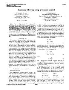
Curve Tracking Control for Legged Locomotion Fumin Zhang Department of Mechanical and Aerospace Engineering, Princeton University [email protected]

Abstract— Recent developments in legged mobile robots call for curve tracking control laws that enable safe movements in complex environment. The lateral leg spring (LLS) model captures planar locomotion dynamics that are platform independent. We derive a hybrid feedback control law for the LLS model so that the center of mass of a legged runner follows a curved path in horizontal plane. The control law enables the runner to change the placement and the elasticity of its legs to move in a desired direction. Stable motion along a curved path is achieved using curvature, bearing and relative distance between the runner and the curve as feedback. Constraints on leg parameters determine the class of curves that can be followed. These results are applicable to a wide range of legged robots.

legged locomotion modeled by the LLS model is a hybrid system. Correspondingly, the tracking control contains a discrete tracking algorithm which guarantees convergence to the desired curve and a continuous law to control the leg parameters of the LLS model. Section II serves as an introduction to the LLS model. The discrete tracking algorithm is developed in Section III. In Section IV, control laws are developed for the leg parameters to enable the discrete tracking algorithm. The constraints on the parameters and the effects on the tracking behavior are discussed in Section V. We provide simulation results in Section VI.

I. I NTRODUCTION

II. M OTION OF THE COM

From tiny ants to large elephants, legged locomotion is the dominant method that animals use to move on the ground. Although the leg structures are vastly different across species, the mechanisms for walking, jumping or running obey strikingly similar principles. These similarities are captured by mathematical models such as the spring-loaded inverted pendulum (SLIP) model, see [1], and the lateral leg spring (LLS) model in [2]–[5]. The LLS model describes motion in the horizontal plane and the SLIP model describes motion in the sagittal (vertical) plane. We use the LLS model in this paper in designing curve tracking control in the horizontal plane; the runner is modeled as a rigid body with two weightless springs attached to a point in the body called the center of pressure (COP). Each spring represents legs on one side of the body. The COP is usually not coincident with the center of mass (COM). Legged locomotions can be self-stabilized—the running or walking gaits stay close to being periodic under disturbances—without feedback control. As indicated by a recent review [6], the self-stabilized walking and running happen when the runner moves along a straight line. There are many interests in engineering practice to design and build legged robots that are versatile on rough terrains. Legged robots are greatly appreciated in applications such as searching and rescuing missions and planet exploration. In most missions, the robots must be able to move along an arbitrary path. Feedback control is needed for tracking curved path as well as stabilizing the periodic gaits. In this paper, we develop feedback control law for the LLS model so that the COM follows a curved path. The

In the horizontal plane, motion generated by the LLS model starts when the free end of one spring (or leg) is placed at a touchdown point P . At this starting moment, the spring is at its free length η0 . If the COM has a non-zero initial velocity v that is not perpendicular to the spring, then the spring will be first compressed to a minimum length and later be restored to its free length. This process, starting and ending with the spring at its free length η0 , is called a stance phase or simply a stance. The COM moves from the starting position to an ending position after a stance. Suppose that mechanical energy is conserved during each stance, then the starting and ending speed of a stance is identical. As shown in Figure 1, the end of one stance serves as the beginning of the next stance with the touchdown point P shifted from one side to the other. This allows us to distinguish left stances from right stances based on which leg is supporting the body. The rigid body moves forward as a result of switching between left and right stances. As shown in Figure 1, we use ri , i = 1, 2, ..., to denote the position of the COM in a lab fixed coordinate frame at the beginning of the ith stance. We use αi to denote the angle between the velocity vi and the spring at rest. For a right stance, the angle is measured counter-clockwise from the spring to the velocity vector. For a left stance, the angle is measured clockwise from the spring to the velocity vector. Under this convention for measuring angles, αi has to be within the interval (0, π/2) to generate forward locomotion. We can view ri as points on a curve Γ which is formed by straight line segments that connects ri−1 with ri for all i. This curve Γ is not the actual trajectory of the COM, but it intersects with the trajectory of the COM at the points ri . We then let qi = ri+1 − ri and define qi = k qi k. We also define an angle δi as the angle between the vector qi

This work was supported in part by ONR grants N00014–02–1– 0826, N00014–02–1–0861 and N00014–04–1–0534. I want to thank Philip Holmes, Justin Seipel and Naomi Leonard for discussions and suggestions.

normal vectors yi and yci as shown in Figure 2. The angle θi between xi and xci is defined by letting cos θi = xi · xci and sin θi = −xi · yci .

(2)

In Figure 2, the closest point on the boundary moves from rci to rci+1 during a stance. We then assume that each stance is short enough so that the curvature of the boundary curve detected during this period can be approximated by a finite constant κi . From Figure 2, we observe β = π2 − θi . Therefore, according to the cosine law, we have 1 2 1 1 ) = (ρi + )2 − 2(ρi + )qi sin θi + qi2 . (3) κi κi κi We can view ρi as state variables, consider qi as the control over step size, and θi as steering control. Equation (3) describes the controlled relative motion between the COM and the detected boundary curve. Suppose that the step size qi has been determined. We need to find θi such that ρi converges to a desired value ρc as i → ∞. If we can find a feedback control law fi (·) such that ρi+1 − ρi = fi (ρi − ρc ), (4) (ρi+1 +

Fig. 1. The LLS model for legged locomotion. One left stance followed by one right stance are plotted. The center of mass (COM) is translated from ri−1 to ri . The velocities of the COM at the beginning of each stance are the vectors vi−1 and vi . The angle between vi and the spring (leg) is αi . The angle between vector qi and the horizontal axis X is δi . The positive directions for all angles are as shown.

and the horizontal axis of the lab frame, measured counterclockwise from the axis. This angle describes the direction of curve Γ for the ith stance. The motion of the COM can now be described by a discrete system ri+1 = ri + [qi cos δi , qi sin δi ]T .

(1)

III. T RACKING A DETECTED BOUNDARY Suppose at the position ri , the runner is able to detect a segment of a boundary curve from sensor information, c.f., [7] and [8]. Suppose the runner is also able to estimate a point on the boundary curve that has the minimum distance to the COM. We call this point the closest point rci shown in Figure 2. By selecting two extra points on the boundary near rci , the runner can estimate the tangent vector to the boundary curve xci and the curvature of the boundary curve κi using algorithms summarized in [7]. Here we suppose all estimates are perfect.

then we can choose the function fi (·) so that ρi − ρc → 0. For example, we may let fi (ρi − ρc ) = −Ki · (ρi − ρc ) where 0 < Ki < 1. Observe that ρi+1 − ρi = ρi+1 − ρc − (ρi − ρc ),

ρi+1 − ρc = (1 − Ki )(ρi − ρc ).

(7)

Since −1 < 1 − Ki < 1, it is true that ρi → ρc as i → ∞. We now define λi = ρi + κ1i . In order to achieve (4), we replace (ρi+1 + κ1i ) with (λi + fi ) in (3). From (3), we can solve for sin θi as = =

We let ρi be the distance between the COM at ri and the closest point at rci . We also let xi = k qqii k be the unit vector in the direction of qi . We can then define two right handed frames—one at ri and the other at rci —by defining two unit

(6)

and this leads to

sin θi

Fig. 2. The movement of the COM near a boundary curve. θi is the angle between qi and xci . ρi is the distance between the COM and the closest point. κi is the curvature of the curve. γi is the center angle of the arc connecting rci and rci+1

(5)

−fi2 − 2λi fi + qi2 2λi qi qi fi f2 − − i . 2λi qi 2λi qi

(8)

When fi = 0, the solution is θi = sin−1 (qi /2λi ). This corresponds to the runner running parallel to the boundary curve. Note that when κi → 0, then λi → ∞. The limit of equation (8) is sin θi = − fqii , which is equivalent to ρi+1 − ρi = −qi sin θi . This equation indeed describes the relative motion between the COM and a straight line. Therefore, all the results that will be obtained from (8) are applicable to straight lines by letting λi → ∞. Lemma 3.1: A solution exists for θi in equation (8) if and only if fi ∈ [−(2λi + qi ), min{−qi , qi − 2λi }] or fi ∈ [max{−qi , qi − 2λi }, qi ]. Proof: A solution exists for θi if and only if −fi2 − 2λi fi + qi2 ≤1 2λi qi

(9)

and

−fi2 − 2λi fi + qi2 ≥ −1. 2λi qi One can verify that these are equivalent to

(10)

−(2λi + qi ) ≤ fi ≤ min{−qi , qi − 2λi }

(11)

max{−qi , qi − 2λi } ≤ fi ≤ qi .

(12)

or

Lemma 3.2: Suppose 0 < qi < 2λi . Let fi = −Ki (ρi − ρc ). There exists Ki ∈ (0, 2) such that (12) is satisfied and θi in (8) has a solution. Proof: If |ρi − ρc | < 21 min{qi , 2λi − qi }, we may let Ki be any value in the interval (0, 2) and (12) is satisfied. If |ρi − ρc | ≥ 12 min{qi , 2λi − qi }, we may let 0 < Ki < min{2,

2λi − qi qi , } |ρi − ρc | |ρi − ρc |

(13)

where we assume the spring has potential energy V which depends only on its length. During each stance, the dynamics can be described as a continuous nonlinear Hamiltonian system; the Hamilton equations are developed in [2]. The system is not integrable when the distance between the COM and the COP is nonzero. In this case numerical methods are necessary to compute the trajectory of the COM from knowledge of the states (η, ψ, σ). To illustrate analytical insights for the tracking problem, it is much easier to study the case when the COP and COM coincide. This is because the corresponding system is integrable. The Hamilton equations for the dynamics of the COM are 1 2 ∂V p − p˙η = mη 3 η ∂η p˙ψ = 0 (16) ˙ where pη = mη˙ and pψ = mη 2 ψ.

which satisfies (12). The condition qi < 2λi in Lemma 3.2 indicates that each step size should not be too big. The following theorem is a direct consequence of Lemma 3.2. Theorem 3.3: Suppose the step size qi satisfy 0 < qi < 2λi . Let fi = −Ki (ρi − ρc ). Select Ki ∈ (0, 2) such that θi in (8) has a solution. Then under the control qi and θi , we have ρi → ρc as i → ∞. Once θi is determined from (8), we can compute the direction of qi in the lab frame. This is because δi = ζi − θi

(14)

where ζi is the angle between the horizontal axis of the lab frame and the vector xci , measured counter clockwise from the horizontal axis. Knowing qi and δi allows us to compute the position of the COM for the next stance from the discrete system given by equation (1). IV. C ONTROL THE LLS MODEL In order to generate desired qi and δi to control the COM movement, the runner needs to change its leg placements or the elasticity of the legs. We investigate the dynamics during each stance to establish the relations between the COM motion and the leg parameters. Leg parameters for a right stance and a left stance often differ only by the sign. Since a right stance is always followed by a left stance and vice versa, we use the convention that the stance k is always a right stance and stance k + 1 is always a left stance. Therefore, stance k + 2 must be a right stance, etc. In the following, we will only show detailed derivation for a right stance; similar results for a left stance will be listed directly. We set up a polar coordinate system at the touchdown point Pk with the horizontal x-axis parallel to the horizontal X-axis of the fixed lab frame. Let (η, ψ) be the polar coordinates of the COM in this frame and let σ describe the orientation of the rigid body. Then the total energy is 1 1 1 E = mη˙ 2 + mη 2 ψ˙ 2 + I σ˙ 2 + V (η) (15) 2 2 2

Fig. 3. The LLS model with COM coincide with COP. Angle φk is the center angle swept during the stance. Angle αk is the angle between the leg and the velocity vk at the moment of touch down.

We plot one right stance in Figure 3. Let vk be the velocity of the COM at the beginning of the kth stance. This vk provides initial value for the states pη and pψ of the system (16). Because mechanical energy is conserved, the speed vk = k vk k satisfies vk+1 = vk . We let αk represent the angle measured from the leg to the velocity vk at the moment of touchdown, and we call αk the leg placement parameter. We use ϕk to measure the direction of velocity in the lab frame. By using simple geometric relationships in Figure 3, we have π φk − − αk = δk − ϕk . (17) 2 2 Therefore, using equation (14), π φk − αk − . (18) 2 2 Note that (ζk −ϕk ) is the relative angle between vk and xck : the tangent vector to the boundary curve at the closest point. We know θk is the angle between vector qk and the same tangent vector xck . Therefore, (ζk − ϕk − θk ) is the angle between vk and qk . From (18), we see that changing αk will change the direction of the COM movement qk . This is also true for a left stance where we have π φk+1 ζk+1 − ϕk+1 − θk+1 = −( − αk+1 − ). (19) 2 2 ζ k − ϕk − θ k =

Another relationship we can derive from Figure 3 is qk = 2ηk sin

φk 2

A. the constraints (20)

where ηk represents the leg length at the moment of touchdown. In (20) and (18), qk is the distance the runner wants to travel in one stance, the angle θk can be solved from (8), and the angle (ζk − ϕk ) is known. We want to solve for the leg parameters αk and ηk , but φk is still unknown. This unknown can be solved from the continuous system equations (16). At the starting position of the kth stance rk and the ending position of the kth stance rk+1 , by conservation of the angular momentum, we have pηk+1 = pηk = ηk2 ψ˙ = ηk vk sin αk .

(21)

To generate forward locomotion, the relative angle αk between the leg and the COM velocity vk should be bounded within the interval (0, π/2). Figure 4 illustrates the possible qk that can be produced by changing αk for a right stance when ηk and bk are held constant. The parameters for the plotted LLS model are m = 2.5g, vk = 0.2m/s, ηk = 1.7cm and bk = 1.05N/m which are typical for a cockroach. When αk = 0 and αk = π/2, we have qk = 0. Therefore, in order to move forward effectively, the angle αk must be within an interval [αmin , αmax ] with αmin > 0 and αmax < π/2. The solid segment in Figure 4 illustrates the possible qk between αmin = π/6 and αmax = π/3. There the maximum qk is 1.44cm. When αk is within [π/6, π/3], the minimum qk is 1.24cm. The changes in qk is not big for a wide range of αk . This is typical for LLS models.

Using the method of integration by quadrature, c.f. [9], we can compute the center swing angle φk for each stance as Z

pηk η2

ηmin

φk = 2 ηk

q ± 2E −

p2η k η2

dη

(22)

− 2V (η)

where ηmin is the shortest length of the spring during the stance. When η = ηmin , we have η˙ = 0. Thus we can solve ηmin from p2η 2E − 2 k − 2V (ηmin ) = 0 . (23) ηmin Since φk is now a known function of αk , ηk , and bk , we can solve for any two of αk , ηk , and bk from (18) and (20) when keeping the other parameter constant. For a runner, controlling αk means to find the appropriate angle between its leg and the direction of the COM motion. On the other hand, as reported by Jindrich and Full in [10], the cockroaches control the length ηk by stretching or compressing their legs when turning. We see that changing ηk will affect both pψk and V (η). This changes φk and hence controls (ζk − ϕk − θk ). Another means of steering is to change the potential energy V (η) ,e.g., change the spring constant bk , which also controls φk . If the conditions in Theorem 3.3 are satisfied, equation (8) always has a solution for θi . The equations (18), (20) and (22) can be solved to implement the control θi . Note that finding solutions for αk and ηk often requires numerical methods because φk is not a simple function of αk and ηk . V. T RACKING B EHAVIOR U NDER C ONSTRAINTS For every stance, the LLS model generates the COM movement qk by controlling parameters such as αk , ηk and bk . In practice, these parameters all have to be bounded. These bounds post constraints on the possible qk that can be generated by the LLS model. In this section, we discuss the constrained COM movement and investigate the constrained tracking behavior when a runner is running along a curve path.

Fig. 4. The possible qk generated by a right stance for an LLS model. vk is the velocity of the COM. The units are in meters. The curve (dotted and solid) illustrates the end points for vector qk starting from the origin when αk changes from 0 to π/2 while other parameters are constant. The solid segment corresponds to αk ∈ [π/6, π/3].

The above example suggests that it is possible to keep ηk , qk and φk constant for each stance. We control the spring constant bk and the leg placement angle αk . The advantage of this strategy is that the distance traveled by the COM is identical for every stance. This fact can help us analyze the tracking behavior later. For the LLS model plotted in Figure 4, in order to keep qk = 1.44cm, we plot the spring constant bk as a function of the leg placement angle αk in Figure 5. For αk ∈ [π/6, π/3], bk lies between 0.78 N/m and 1.06 N/m. This range is not difficult to implement. With qk constant for each stance, the possible movement of the COM can be depicted by a cone Ck . The two edges of the cone correspond to αk = αmin and αk = αmax . The length of both edges are qk . Figure 6 illustrates cone Ck+1 and cone Ck . Ck+1 grows from the end point of qk which lies in the circular arc of Ck . We found that Ck+1 is the mirror image of Ck with qk being the axis of symmetry. This is because the velocity vector vk+1 and vk are symmetric with respect to qk , which can be proved by solving equations (16). Therefore, as the runner moves forward, the cone will flip from side to side.

1.2

1.1

1

0.9

0.8

0.7

0.6

0.5

0.4

0.3

0.2

0

0.2

0.4

0.6

0.8

1

1.2

1.4

Fig. 5. The spring constant bk (in N/m) as a function of leg placement angle αk (in radians) to keep qk = 1.44 cm. The solid segment corresponds to αk ∈ [π/6, π/3].

Fig. 6. The cones flip from one side to another when running. On the left, the cones Ck and Ck+1 are symmetric with respect to qk which is the solid arrow. In the middle, the runner is running along a straight line. On the right, the runner is running along a curve path in the counter clockwise direction.

B. running along a curve path and robustness We use the index i for all right and left stances. When running parallel to a desired curved path, the COM movement satisfies ρi = ρc for all i. Therefore, we have fi = 0 in equation (8). The following conditions are necessary: A1) qi ∈ Ci ; A2) θi = sin−1 (qi /2λi ). Condition A1 requires that the COM movement belongs to the cone that is feasible for the constrained model. Condition A2 requires that qi is parallel to the desired curve.

B . q is the middle line of C A , and Fig. 7. The sub-cones CkA and Ck+1 k k qk+1 is the middle line of CkA . The angle difference between qk+1 and qk is γ.

If the desired curve is a straight line segment, then θi = 0 in condition A2. As the runner moving forward, the cone Ci will be flipping side to side with respect to the straight line. In this case we have αi = αi+1 . The robustness of this behavior is determined by the size of the cone and the

value of αi . If we choose the value of αi so that the COM movement qk is always in the middle of the cone, then the tracking behavior is the most robust. See the middle figure in Figure 6. If the desired curve is convex with positive curvature, then θi 6= 0. To find out θi , we study the kth and (k +1)th stance, i.e., a right stance followed by a left stance. For convenience we let qk . (24) γk = 2 sin−1 2λk Observe from Figure 2 that θk+1 − θk = −(αk+1 − αk ) + γk .

(25)

Condition A2 implies that θk+1 = θk = γk /2. Therefore, when running along a convex curve, αk+1 − αk = γk should be satisfied. We have similar relation for stance k + 1 and k + 2, i.e., a left stance followed by a right stance: αk+2 − αk+1 = −γk+1 . We can then write αi+1 − αi = ±γi for all stances. This equation requires that γi must be less than (αmax −αmin ). This implies that λi , the instantaneous radius of the curve must satisfy qi . (26) λi > min 2 sin αmax −α 2 This condition is stricter than λi > qi /2 required by Lemma 3.2. Hence the constraint on αi puts a tighter restriction on the curvature of the curve that can be traced. We divide Ci into two sub-cones. Let CiA be the cone for α ∈ [αmin , αmax − γi ]. Let CiB be the cone for α ∈ [αmin + γi , αmax ]. Because Ci flips and αi+1 − αi = ±γi , if B qi belongs to CiA , then qi+1 belongs to Ci+1 . Now consider a right stance k followed by a left stance (k+1). When running along a convex curve in the counter clockwise (CCW) B , direction, the runner must have αk ∈ CkA and αk+1 ∈ Ck+1 see Figure 7. When running in the clockwise (CW) direction, A the runner must have αk ∈ CkB and αk+1 ∈ Ck+1 . To increase the robustness of the tracking behavior, we should let the COM movement qi be close to the middle of Ci . In the case of convex curves, the best choice is to let qi and qi+1 be symmetric with respect to the middle line of Ci . The middle lines of CiA and CiB are symmetric with respect to the middle line of Ci . The angle between the middle lines of CiA and CiB is γi . If the curve has constant curvature, then γi is constant for all i. This implies that the middle lines of B CiA and Ci+1 are symmetric with respect to the middle line of Ci . Therefore, we may choose qi to be the middle line of either CiA or CiB for maximum robustness. If the curve has a changing positive curvature, then γi can be different from stance to stance. This “middle line” strategy can not be enforced. In this case one can choose qi to be as close to the middle lines as possible. If the desired curve is not convex, the tracking behavior can be viewed as switching between tracking a locally convex curve in the CCW direction and in the CW direction. The switching depends on how the curve changes from locally convex to locally concave. No general conclusions can be drawn regarding which part of the cone Ci is used

for a stance. In this case the tracking behavior is not a “steady state” . VI. S IMULATIONS We present simulation results to demonstrate tracking a circle centered at the origin with radius 0.02m. The parameters for the LLS model are the same as in section V. The desired distance to the circle is 0.03m. Initially, the runner start from (0.1, 0) outside the circle. The speed of the COM is 0.2m/s. The initial direction of the velocity is π/3. The leg placement angle αi are constrained to be within the interval (π/6, π/3). We change the spring constant bk so that qi is always equal to 1.53cm, which is 90% of the leg length at rest.The gain Ki is selected to be 0.5. When θi can not be achieved by αi , we simply use the value for αi that will minimize the differences between desired θ˜i and achievable θi ; hence implemented the approximation method. The trajectory of the COM and the distance between the COM and the circle are plotted in Figure 8. We see that the convergence is achieved after 12 stances which take less than one second.

(a) trajectory of COM

(b) distance between COM and the circle Fig. 8. Tracking a circle with radius 0.02m. In (a), the cross symbols indicate the touchdown points. The units for both horizontal and vertical axis are meters. In (b), the distance (in meters) between the COM and the circle is plotted as a function of time (in seconds). We can see it converges to the desired separation 0.03m.

VII. S UMMARY AND F UTURE W ORK We have analyzed the control of LLS model and designed a hybrid curve tracking control law for legged locomotion.

Using measurements of the curve for feedback, the discrete algorithm guarantees convergence to the desired curve path. During each stance, the controlled continuous dynamics is analyzed. The parameters of the LLS model is determined to implement the discrete algorithm at the beginning of each stance. We have also investigated the effects of parameter constraints. These constraints limited tracking ability. For straight lines and convex curves, a steady state can be reached. The robustness of these steady states depends on the range for the parameters. Interesting results regarding wall following behaviors of cockroaches are reported by Camhi and Johnson in [11]. Recently, a wall following wheeled robot using antenna like tactile sensor was reported in [8]; curve tracking for atomic force microscope is discussed in [12]; a general boundary tracking control law is derived for Newtonian particles in [13]. Our work, although intended for legged locomotion, may be adapted to handle other cases, for example, locomotions with flapping wings [14]. R EFERENCES [1] R. Full and D. E. Koditschek, “Templates and anchors: Neuralmechanical hypothesis of legged locomotion on land,” Journal of Experimental Biology, vol. 83, pp. 3325–3332, 1999. [2] J. Schmitt and P. Holmes, “Mechanical models for insect locomotion: Dynamics and stability in the horizontal plane I. Theory,” Biological Cybernetics, vol. 83, pp. 501–515, 2000. [3] ——, “Mechanical models for insect locomotion: Dynamics and stability in the horizontal plane II. Applications,” Biological Cybernetics, vol. 83, pp. 517–527, 2000. [4] ——, “Mechanical models for insect locomotion: Stability and parameter studies,” Physica D, vol. 156, pp. 139–168, 2001. [5] J. Schmitt, M. Garcia, R. Razo, P. Holmes, and R. J. Full, “Dynamics and stability of legged locomotion in the horizonatoal plane: A test case using insects,” Biological Cybernetics, vol. 86, pp. 343–353, 2002. [6] R. M. Ghigliazza, R. Altendorfer, P. Holmes, and D. Koditschek, “A simply stablized running model,” SIAM Review, vol. 47, no. 3, pp. 519–549, 2005. [7] F. Zhang, A. O’Connor, D. Luebke, and P. S. Krishnaprasad, “Experimental study of curvature-based control laws for obstacle avoidance,” in Proc. 2004 IEEE International Conf. on Robotics and Automation, New Orleans, LA, 2004, pp. 3849–3854. [8] A. G. Lamperski, O. Y. Loh, B. L. Kutscher, and N. J. Cowan, “Dynamical wall-following for a wheeled robot using a passive tactile sensor,” in Proc. 2005 IEEE International Conf. on Robotics and Automation, Barcelona, Spain, 2005, pp. 3838–3843. [9] V. Arnold, Mathematical Methods of Classical Mechanics 2nd Ed. New York: Springer, 1989. [10] D. Jindrich and R. J. Full, “Many legged maneuverability: dynamics of turning in hexapods,” Journal on Experimental Biology, vol. 202, pp. 1603–1623, 1999. [11] J. M. Camhi and E. N. Johnson, “High-frequency steering maneuvers mediated by tactile cues: Antennal wall-following in the cockroach,” Journal of Experimental Biology, vol. 202, pp. 631–643, 1999. [12] S. B. Andersson and J. Park, “Tip steering for fast imaging in AFM,” in Proc. 2005 American Control Conf., Portland, OR, June 6-10, 2005, pp. 2469–2474. [13] F. Zhang, E. Justh, and P. S. Krishnaprasad, “Boundary following using gyroscopic control,” in Proc. 43rd IEEE Conf. on Decision and Control, Atlantis, Paradise Island, Bahamas, 2004, pp. 5204–5209. [14] S. D. Ross, “Optimal flapping strokes for self-propulsion in a perfect fluid,” in Proc. 2006 American Control Conf. Minneapolis, MN: IEEE, 2006, pp. 4118–4122.