Therefore, we propose a new domain for separation of primaries and multiples via the ... have been made to address this problem by either extending move-out.
Curvelet-domain multiple elimination with sparseness constraints Felix J. Herrmann1 and Eric Verschuur2 Department of Earth and Ocean Sciences, University of British Columbia, Canada 2 Faculty of Applied Sciences, Delft University of Technology, The Netherlands 1
Abstract Predictive multiple suppression methods consist of two main steps: a prediction step, in which multiples are predicted from the seismic data, and a subtraction step, in which the predicted multiples are matched with the true multiples in the data. The last step appears crucial in practice: an incorrect adaptive subtraction method will cause multiples to be sub-optimally subtracted or primaries being distorted, or both. Therefore, we propose a new domain for separation of primaries and multiples via the Curvelet transform. This transform maps the data into almost orthogonal localized events with a directional and spatialtemporal component. The multiples are suppressed by thresholding the input data at those Curvelet components where the predicted multiples have large amplitudes. In this way the more traditional filtering of predicted multiples to fit the input data is avoided. An initial field data example shows a considerable improvement in multiple suppression.
Introduction In complex areas move-out filtering multiple suppression techniques may fail because underlying assumptions are not met. Several attempts have been made to address this problem by either extending move-out discrimination methods towards 3D complexities (e.g. by introducing apex-shifted hyperbolic transforms [9]) or by coming up with matching techniques in the wave-equation based predictive methods [see e.g. 19, 1]. Least-squares matching the predicted multiples in time and space overlapping windows, [18] provides a straightforward subtraction method, where the predicted multiples are matched to the true multiples for 2-D input data. Unfortunately, this matching procedure fails when the underlying 2D assumption are severely violated. There have been several attempts to address this issue and the proposed solutions range from including surrounding shot positions [13] to methods based on model- [16], data-driven [12] time delays and separation of predicted multiples into (in)-coherent parts [14]. Even though these recent advances in adaptive subtraction and other techniques have improved the attenuation of multiples, these methods continue to suffer from (i) a relative strong sensitivity to the accuracy of the predicted multiples; (ii) creation of spurious artifacts or worse (iii) a possible distortions of the primary energy. For these situations, subtraction techniques based on a different concept are needed to complement the processor’s tool box. The method we are proposing here holds the middle between two complementary approaches common in multiple elimination: prediction in combination with subtraction and filtering [17, 9]. Whereas the first approach aims to predict the multiples and then subtract, the second approach tries to find a domain in which the primaries and multiples separate, followed by some filtering operation and reconstruction. Our method is not distant from either since it uses the predicted multiples to non-linearly filter data in a domain spanned by almost orthogonal and local basis functions. We use the recently developed Curvelet transform [see e.g. 3], that decomposes data into basis functions that not only obtain optimal sparseness on the coefficients and hence reduce the dimensionality of the problem but which are also local in both location and angle/dip, facilitating the definition of non-linear estimators based on thresholding. Main assumption of this proposal is that multiples and primaries have locally a different temporal, spatial and dip behavior, and therefore map into different areas in the Curvelet domain. Multiples give
rise to large Curvelet coefficients in the input and these coefficients can be muted by our estimation procedure when the threshold is set according to the Curvelet transform of the predicted multiples. As such, our suppression technique has at each location in the transformed domain one parameter, namely the threshold yielded by the predicted multiple, beyond which the input data is suppressed. In that sense, our procedure is similar to the ones proposed by [20] and [17], although the latter use the non-localized FK/Radon domains for their separation while we use localized basis functions and non-linear estimation by thresholding. Non-locality and non-optimality in their approximation renders the first filtering techniques less effective because primaries and multiples will still have a considerable overlap. The Curvelet transform is able to make a local discrimination between interfering events with different temporal and spatial characteristics.
The inverse problem underlying adaptive subtraction Virtually any linear problems in seismic processing and imaging can be seen as a special case of the following generic problem: how to obtain m form data d in the presence of (coherent) noise n: d = Km + n,
(1)
in which, for the adaptive subtraction problem, K and K∗ , represent the respective time convolution and correlation with an effective wavelet Φ that minimizes the following functional [see e.g. 8] t
min = kd − Φ ∗ mkp , Φ
(2)
where d represents data with multiples; m the predicted multiples and ˆ = minΦ kd − Φ ∗ mkp the primaries only data, obtained by minin mizing the Lp -norm. For p = 2, Eq. 2 corresponds to a standard leastsquares problem where the energy of the primaries is minimized. Seismic data and images are notoriously non-stationary and nonGaussian, which may give rise to a loss of coherent events in the denoised component when employing the L2 -norm. The non-stationarity and non-Gaussianity have with some success been addressed by solving Eq. 2 within sliding windows and for p = 1 [8]. In this paper, we follow a different strategy replacing the above variational problem by m ˆ :
1 −1/2 (d − m) k22 + µJ(m). min kCn m 2
(3)
In this formulation, the necessity of estimating a wavelet, Φ has been omitted. Data with multiples is again represented by d but now m is the primaries only model on which an additional penalty function is imposed, such as a L1 -norm, i.e. J(m) = kmk1 . The noise term is now given by the predicted multiples and this explains the emergence of the covariance operator, whose kernel is given by Cn = E{nnT }.
(4)
Question now is can we find a basis-function representation which is (i) sparse and local on the model (primaries only data), m, data, d and predicted multiples n and (ii) almost diagonalizes the covariance of the model and the predicted multiples. Answer is affirmative, even
though the condition of locality is non-trivial. For instance, decompositions in terms of principle components/Karhuhnen-Lo´eve-basis (KL) or independent components may diagonalize the covariance operators but these decomposition are generally not local and not necessary the same for both multiples and primaries. By selecting a basis-function decomposition that is local, sparse and al2 most diagonalizing (i.e. Cn ˜ ≈ diag{Cn ˜ } = diag{Γn ˜ }), we find a solution for the above denoising problem that minimizes (mini) the maximal (max) mean-square-error given the worst possible Bayesian prior for the model [15, 7]. This minimax estimator minimizes j/2
m ˆ0 :
� � 1 ˜−m ˜ k22 min kΓ−1 d n ˜ m 2
c2
(5)
2-j
basis functions
by a simple diagonal non-linear thresholding operator -j/2
� � � ˜ . m ˆ = B† ΓΘλ Γ−1 Bd = B† ΘλΓ d
c2
(6)
The threshold is set to λdiag{Γ} (we dropped the subscript n ˜ ) with λ an additional control parameter, which sets the confidence interval (e.g. the confidence interval is 95 % for λ = 3) (de)-emphasizing the thresholding. This thresholding operation removes the bulk of the multiples by shrinking the coefficients that are smaller then the noise to zero. The symbol † indicates (pseudo)-inverse, allowing us to use Frames rather then orthonormal bases. Before applying this thresholding to actual data, let us first focus on the selection of the appropriate basis-function decomposition that accomplishes the above task of replacing the adaptive subtraction problem given in Eq. 2 by its diagonalized counterpart (cf. Eq. 6).
The basis functions
2-j wavelet
curvelet
Fig. 1: Top left: Curvelet partitioning of the frequency plane [modified from [5]]. Bottom right: Comparison of non-linear approximation rates Curvelets and Wavelets [modified from [6]].
Curvelets live in a wedges of the 2-D Fourier plane and become more directional selective and anisotropic for the higher frequencies. They are localized in both the space (or (x, t)) and spatial KF-domains and have, as consequence of their partitioning, the tendency to align themselves with curves/wavefronts. As such they are more flexible then a representation yielded by high-resolution Radon [as described by e.g. 17] because they are local and able to follow any piece-wise smooth curve. In Figure 1, a number of Curvelet properties are detailed [adapted from [5, 3, 6]].
Curvelets as proposed by [3], constitute a relatively new family of non-separable wavelet bases that are designed to effectively represent seismic data with reflectors that generally tend to lie on piece-wise smooth curves. This property makes Curvelets suitable to represent events in seismic whether these are located in shot records or time slices. For these type of signals, Curvelets obtain nearly optimal sparseness, because of (i) the rapid decay for the reconstruction error as a function of the largest coefficients; (ii) the ability to concentrate the signal’s energy in a limited number of coefficients; (iii) the ability to map noise and signal to different areas in the Curvelet domain. So how do Curvelets obtain such a high non-linear approximation rate? Without being all inclusive [see for details 4, 2, 3, 6], the answer to this question lies in the fact that Curvelets are
As the examples in the next section clearly demonstrate, the optimal denoising capabilities for incoherent noise carry over to coherent noise removal provided we have reasonable accurate predictions for the noise, the multiples in this case. By choosing a threshold defined by the predicted multiples, i.e. Γ = λ|Bn|, (7)
• multi-scale, i.e. they live in different dyadic corona (see for more detail [3] or the other contributions of the first author to the proceedings of this conference) in the FK-domain.
The above methodology is tested on a field dataset from offshore Scotland. This is a 2D line, which is known to suffer from strong surfacerelated multiples. Because the geology of the shallow sub-bottom layers is laterally complex, multiples have been observed to exhibit 3D characteristics. Applying surface-related multiple elimination to this data gives only an attenuation of surface multiples, but not a complete suppression. This lack of suppression can be observed for a shot record shown in Fig. 2. When comparing the predicted multiples with the input data a good resemblance is observed in a global sense. However, when a matching filter is calculated, it appears that the predicted multiples do not coincide well enough with the true multiples, mainly due to 3D effects. Locally the temporal and spatial shape of the predicted multiples - especially for the higher order multiples - differs from the true events. Estimating shaping filters in spatially and temporally varying, overlapping windows, as described by [18] can not resolve this mismatch completely. The adaptive subtraction result is displayed in Fig. 2 in the third panel. To improve this result, more freedom can be incorporated in the subtraction process. However, note that the more the predicted multiples
• multi-directional, i.e. they live on wedges within these corona. See Fig. 1. • anisotropic, i.e. they obey the following scaling law width ∝ length2 . • directional selective with # orientations ∝
√1 . scale
• local both in (x, t)) and KF. • almost orthogonal, they are tight frames with a moderate redundancy. Contourlets implement the pseudo-inverse in closed-form while Curvelets provide the transform and its adjoint, yielding a pseudo-inverse computed by iterative Conjugate Gradients.
we are able to awe are able to adaptively decide whether a certain event belongs to primary or multiple energy. The n contains the predicted multiples and λ represents an additional control parameter which sets the confidence interval (de)-emphasizing the thresholding.
Results of SRME with thresholding
can adapt to the input data, the higher the chance that primary energy will be distorted as well, as the primary and multiple energy are not orthogonal to each other in the least-squares sense. Multi-gather subtraction using 9 surrounding multiple panels gives better suppression of the multiples but leaves a lot of multiple remnants to be observed, especially for the large offset at large travel times. The output gather of the Curvelet method (see fourth panel in Fig. 2) looks much cleaner. Furthermore, clear events have been restored from interference with the multiples in the lower left area. Also note the good preservation of a primary event around -1000 meter offset and 1.1 seconds. The amplitudes seem to be identical to the ones in the input data, whereas the adaptive subtraction has distorted these amplitudes to some extend. For the Curvelet-domain procedure, the threshold value can be set by the user, thus creating more or less suppression. Too weak thresholding leaves too much multiples in the data and that a too strong thresholding procedure seems to remove too much energy. The filtering via the Curvelet domain can also be applied within each 2D cross-section through the seismic data volume. Time slices at t = 1.48 through the prestack shot-offset data and predicted-multiple volumes are displayed in Fig. 3 (top row). Results after application of the adaptive subtraction per shot record and the time-slice only Curvelet subtraction are included in Fig. 3 (bottom row). Again, the Curvelet results look much cleaner than the least-squares subtraction result. Much of the noisy remnants at small offsets in the least-squares subtraction result have been removed. Notice also the improved suppression of the higher order peglegs in the area around shot 900 and offset 1500 meter.
Conclusions In this paper a new concept related to multiple subtraction has been described, based on the Curvelet transform. The Curvelet transform is an almost orthogonal transformation into local basis functions parameterized by their relate temporal- and spatial-frequency content. Because of their anisotropic shape, Curvelets are directional selective, i.e. they have local angle-discrimination capabilities. Our method uses the predicted multiples from the surface-related multiple prediction method, as a guide to suppress the Curvelet coefficients related to the multiple events directly in the original data. Therefore, the multiples are not actually subtracted, but areas in the Curvelet domain related to multiple energy are muted. The success of this method depends on the assumption that primaries and multiples map into different areas in the Curvelet domain. Based on a field data example, we can conclude that the Curvelet-based multiple filtering is effective and is able to suppress multiples, while preserving primary energy. Especially in situations with clear 3D effects in the 2D seismic data, it appears to perform better than the more traditional least-squares adaptive subtraction methods. This success does not really come as a surprise given the successful application of these techniques to the removal of noise colored by migration [10, 11] and to the computation of 4D difference cubes (see for details in both other contributions of the first to proceedings of this conference). Leaves us to hope for future higher dimensional implementation of the Curvelet transform possibly supplemented by constraint optimization imposing sparseness constraints (see the migration paper in these proceedings).
Acknowledgments The authors thank Elf Caledonia Ltd (now part of Total) for providing the field data and Emmanuel Cand´es and David Donoho for making an early version of their Curvelet code (Digital Curvelet Transforms via Unequispaced Fourier Transforms, presented at the ONR Meeting, University of Minnesota, May, 2003) available for evaluation. This work was in part financially supported by a NSERC Discovery Grant.
References [1] A. J. Berkhout and D. J. Verschuur. Estimation of multiple scatter-
[2]
[3]
[4]
[5]
[6] [7]
ing by iterative inversion, part I: theoretical considerations. Geophysics, 62(5):1586–1595, 1997. E. J. Cand`es and David Donoho. New tight frames of curvelets and optimal representations of objects with smooth singularities. Technical report, Stanford, 2002. URL http://www.acm. caltech.edu/˜emmanuel/publications.html. submitted. E. J. Cand`es and F. Guo. New multiscale transforms, minimum total variation synthesis: Applications to edgepreserving image reconstruction. Signal Processing, pages 1519–1543, 2002. URL http://www.acm.caltech.edu/ ˜emmanuel/publications.html. Emmanual J. Cand`es and David L. Donoho. Curvelets – a surprisingly effective nonadaptive representation for objects with edges. Curves and Surfaces. Vanderbilt University Press, 2000. Emmanual J. Cand`es and David L. Donoho. Recovering Edges in Ill-posed Problems: Optimality of Curvelet Frames. Ann. Statist., 30:784–842, 2000. M. Do and M. Vetterli. Beyond wavelets, chapter Contourlets. Academic Press, 2002. David L. Donoho and Iain M. Johnstone. Minimax estimation via wavelet shrinkage. Annals of Statistics, 26(3):879–921, 1998. URL citeseer.nj.nec.com/donoho92minimax.html.
[8] A. Guitton. Adaptive subtraction of multiples using the l1 -norm. Geophys Prospect, 52(1):27–27, 2004. URL http://www.blackwell-synergy.com/links/doi/ 10.1046/j.1365-2478.2004.00401.x/abs. [9] N. Hargreaves, B. verWest, R. Wombell, and D. Trad. Multiple attenuation using apex-shifted radon transform. pages 1929–1932, Dallas, 2003. SEG, Soc. Expl. Geophys., Expanded abstracts. [10] Felix J. Herrmann. Multifractional splines: application to seismic imaging. In Andrew F. Laine; Eds. Michael A. Unser, Akram Aldroubi, editor, Proceedings of SPIE Technical Conference on Wavelets: Applications in Signal and Image Processing X, volume 5207, pages 240–258. SPIE, 2003. URL http://www.eos. ubc.ca/˜felix/Preprint/SPIE03DEF.pdf. [11] Felix J. Herrmann. Optimal seismic imaging with curvelets. In Expanded Abstracts, Tulsa, 2003. Soc. Expl. Geophys. URL http: //www.eos.ubc.ca/˜felix/Preprint/SEG03.pdf. [12] L. T. Ikelle and S. Yoo. An analysis of 2D and 3D inverse scattering multiple attenuation. pages 1973–1976, Calgary, 2000. SEG, Soc. Expl. Geophys., Expanded abstracts. [13] H. Jakubowicz. Extended subtraction of multiples. Private communication, Delft, 1999. [14] M. M. N. Kabir. Weighted subtraction for diffracted multiple attenuation. pages 1941–1944, Dallas, 2003. SEG, Soc. Expl. Geophys., Expanded abstracts. [15] S. G. Mallat. A wavelet tour of signal processing. Academic Press, 1997. [16] W. S. Ross. Multiple suppression: beyond 2-D. part I: theory. Delft Univ. Tech., pages 1387–1390, Dallas, 1997. Soc. Expl. Geophys., Expanded abstracts. [17] D. O. Trad. Interpolation and multiple attenuation with migration operators. Geophysics, 68(6):2043–2054, 2003. [18] D. J. Verschuur and A. J. Berkhout. Estimation of multiple scattering by iterative inversion, part II: practical aspects and examples. Geophysics, 62(5):1596–1611, 1997. [19] D. J. Verschuur, A. J. Berkhout, and C. P. A. Wapenaar. Adaptive surface-related multiple elimination. Geophysics, 57(9):1166– 1177, 1992. [20] B. Zhou and S. A. Greenhalgh. Wave-equation extrapolation-based multiple attenuation: 2-d filtering in the f-k domain. Geophysics, 59(10):1377–1391, 1994.
300
400
500
600
shot number 700 800
900
1000
1100
1200
300
400
500
600
shot number 700 800
900
1000
1100
1200
300
400
500
600
shot number 700 800
900
1000
1100
1200
300
400
500
600
shot number 700 800
900
1000
1100
1200
500
offset (m) -3000-2500-2000-1500-1000 -500 0
0.2
0.2
0.5
0.5
0.8
0.8
1.0
1.0
offset (m)
1000
offset (m) -3000-2500-2000-1500-1000 -500 0
1500 2000 2500 3000
500
1.2 1000
1.5
1.5
1.8
1.8
2.0
2.0
2.2
2.2
2.5
2.5
offset (m)
1.2
time (s)
time (s)
3500
1500 2000 2500 3000 3500
offset (m) -3000-2500-2000-1500-1000 -500 0
0.2
0.2
0.5
0.5
0.8
0.8
1.0
1.0
500 1000
offset (m)
offset (m) -3000-2500-2000-1500-1000 -500 0
1500 2000
1.2
time (s)
3000
1.2
3500
1.5
1.5
1.8
1.8
500
2.0
2.0
1000
2.2
2.2
2.5
2.5
offset (m)
time (s)
2500
1500 2000 2500
Fig. 2: Comparison between adaptive least-squares (using time and space varying least-squares filters)and Curvelet subtraction of predicted multiples for one shot record. Input data (left), predicted multiples (second), least-squares subtraction (third) and the results by thresholding Curvelet (right).
3000 3500
Fig. 3: Time slice through the prestack data volume of all shot records. Top: Time slice through the input data with all multiples. Second: Slice through the 2D predicted surface-related multiples. Third: Time slice through the shot records after adaptive subtraction per shot record of the predicted multiples. Bottom: The Curvelet equivalent of the adaptive subtraction computed for a single time horizon.