Deep Feature Selection: Theory and Application to ... - Semantic Scholar

Deep Feature Selection: Theory and Application to Identify Enhancers and Promoters Yifeng Li, Chih-Yu Chen, and Wyeth W. Wasserman Centre for Molecular Medicine and Therapeutics University of British Columbia 950 West 28th Avenue, Vancouver, BC V5Z 4H4 Canada {yifeng,juliec,wyeth}@cmmt.ubc.ca

Abstract. Sparse linear models approximate target variable(s) by a sparse linear combination of input variables. The sparseness is realized through a regularization term. Since they are simple, fast, and able to select features, they are widely used in classification and regression. Essentially linear models are shallow feed-forward neural networks which have three limitations: (1) incompatibility to model non-linearity of features, (2) inability to learn high-level features, and (3) unnatural extensions to select features in multi-class case. Deep neural networks are models structured by multiple hidden layers with non-linear activation functions. Compared with linear models, they have two distinctive strengths: the capability to (1) model complex systems with non-linear structures, (2) learn high-level representation of features. Deep learning has been applied in many large and complex systems where deep models significantly outperform shallow ones. However, feature selection at the input level, which is very helpful to understand the nature of a complex system, is still not well-studied. In genome research, the cis-regulatory elements in non-coding DNA sequences play a key role in the expression of genes. Since the activity of regulatory elements involves highly interactive factors, a deep tool is strongly needed to discover informative features. In order to address the above limitations of shallow and deep models for selecting features of a complex system, we propose a deep feature selection model that (1) takes advantages of deep structures to model non-linearity and (2) conveniently selects a subset of features right at the input level for multi-class data. We applied this model to the identification of active enhancers and promoters by integrating multiple sources of genomic information. Results show that our model outperforms elastic net in terms of size of discriminative feature subset and classification accuracy. Key words: deep learning, feature selection, enhancer, promoter

1

Introduction

Sparse regularized linear models are widely used in machine learning and bioinformatics for classification and regression. These models are shallow feed-forward neural networks which approximate the response variable by a sparse superposition of input variables (or features), that is y ≈ f (x) = xT w + b. From a

2

Y. Li, C.-Y. Chen, and W.W. Wasserman

maximum a posteriori (MAP) estimation (or regularization) perspective, its optimization can be generally formulated to minw,b f (w, b) = l(w, b) + λr(w), where l(w, b) is a loss function corresponding to the negative log-likelihood of data, and r(w) is a sparse regularization term corresponding to the prior of model parameter. Typical loss functions include 0-1 loss, hinge loss, logistic loss (for classification), squared loss (for both classification and regression), εsensitive loss (for regression), etc. A regularization term aims to reduce model complexity, thus avoids overfitting. Also, a sparse regularization can help to select features by taking features with nonzero weights in w. Commonly used sparse regularization terms include l1 -norm (LASSO) [24], non-negativity [16], and SCAD [5]. Perhaps LASSO and its variant, elastic net [28] (as formulated in Equation (1)), are the most popularly used techniques. ( LASSO: r(w) = kwk1 (1) 2 elastic net: r(w) = 1−α 2 kwk2 + αkwk1 LASSO is a special case of elastic net by setting α = 1. The popularity of sparse linear models is due to the reasons as follows. First, their concept is easy to understand. Second, variables can be selected. Third, the learning of model parameter θ is often convex in the parameter landscape, thus many fast implementations are available. However, linear models have three main limitations. (1) Non-linear correlation among variables can not be considered (except by handcrafted features or a kernel extension). (2) High-level representation of features can not be learned due to the shallow structure. (3) There does not exist a “natural” way to extend a two-class linear model to multi-class case in classification and feature selection. Two common multi-class extensions are one-versus-one and one-versus-rest. The corresponding feature selection is accomplished by taking the union of results generated by two-class linear models. For instance, given C classes, softmax regression (a one-versus-rest multi-class extension of logistic regression, see Fig. 1a) with LASSO will produce C subsets of class-specific features. These subsets are then pooled as the final result. Since the final subset of features depends on one specific strategy of multi-class extension, different strategies may yield different results. Through piling up hidden layers, deep neural networks are able to model nonlinearity of features. Fig. 1c is an example of such a deep model called multilayer perceptrons (MLP) which is a deep feed-forward neural network. The techniques of learning deep models and their inferences fall into an active research frontier – deep learning [10], which has four attractive strengths for applying it to complex intelligent systems: First, deep models often dramatically increase prediction accuracy. Second, they can model processes of complex systems. Third, they can generate structured high-level representation of features which can help the interpretation of data. Fourth, (convolutional) deep learning models are robust to temporal or spatial variation. But the learning of such models are usually non-convex in optimization, and the back-propagation algorithm (a first-order method) does not perform well on deeper structures. The optimization strategy using greedy layer-wise unsupervised pretraining and finetuning, proposed

Deep Feature Selection

3

in [10], is considered as a breakthrough. While high-level feature extraction and representation have been intensively studied in the surge of deep learning research [3], feature selection at the input level is still not well-studied. However, in bioinformatics and other studies on complex systems, selecting key input features are crucial to understand the mechanisms of the systems. Thus, existing models mentioned above do not meet this need. In our current bioinformatics research, we are committed to devising a deep learning model for the identification and understanding of cis-regulatory elements in the human genome. Genome researchers have discovered that non-coding DNA sequences (previously viewed as junk DNA) are composed of many regulatory elements [22]. These elements (including enhancers and promoters) precisely control the expression level of genes. Promoters are cis-acting DNA sequences that switch on or off the expression of genes, while enhancers are generally cis-acting DNA sequences that tune the expression level of genes [21]. A promoter resides closely to its target gene, while an enhancer is distal to its target gene(s) making it difficult to identify. The identification of active enhancers and promoters in a genome is of key importance, as it can help to elucidate the regulatory mechanism in the genome, and interpret disease-causing variants within cis-regulatory elements. However, since the regulatory landscapes of DNA are quite different among cell types, and the regulatory events are precisely and dynamically controlled by multiple factors, including epigenetic marks, transcription factors, microRNAs, and their interactions, it is a difficult task to identify active enhancers and promoters in a given cell type. The emergence of both deep sequencing and deep computing techniques casts light on this problem. In order to select key input features for the identification and understanding the regulatory events, we propose a deep feature selection model that enables variable selection for deep neural networks. In this model, a sparse one-to-one layer, where each input feature is weighted, is added between the input and the first hidden layer, giving two advantages: (1) a single subset of features for multiple classes (multiple output nodes) can be conveniently selected, which addresses the challenge of multi-class extension of linear models; (2) through selecting features at the input level of the deep structure, we are able to identify informative features that have non-linear behaviours.

2 2.1

Method Deep Feature Selection

We focus our research on feature selection for multi-class data using deep neural networks. We propose a deep feature selection (DFS) model that can select features at the input level of a deep network. An example of such a model is illustrated in Fig. 1d. Our main idea is to add a sparse one-to-one linear layer between the input layer and the first hidden layer of a MLP. In this one-to-one layer, the input feature xi only connects to the i-th node with linear activation function. Thus, the output of the one-to-one layer becomes w ∗ x, where ∗ is element-wise multiplication. In order to select input features, w has to be sparse,

4

Y. Li, C.-Y. Chen, and W.W. Wasserman

and only the features corresponding to nonzero weights are selected. Although we can resort to any  sparse regularization  term on w. In our current study, we 1−λ2 2 use elastic-net λ1 2 kwk2 + λ2 kwk1 [28]. Such a DFS model can be called deep elastic net. As in regular MLP, the activation function in the hidden layers of DFS is also nonlinear (e.g. sigmoid or tangent). The output layer is a softmax (K+1) T

layer, where the output of unit i is defined as p(y = i|x) =

e−wi PC

c=1

h(K)

(K+1) T (K) h e−wc

,

(K+1)

where wi is the i-th column of weight matrix W (K+1) from the last hidden layer (that is the K-th hidden layer) to the softmax layer. Our DFS model has at least two distinctive advantages. First, given a parameter setting, it always selects a single subset of features for multi-class problems. It overcomes the limitation of linear models for multi-class data making feature selection more convenient. Second, by using a deep nonlinear structure, it can automatically identify non-linear features, which is superior over shallow linear models.

o

Output Layer

o

Output Layer

W Weighted Input (Layer)

W

w*x

w

x

Input (Layer)

(a) Elastic Net

x

Input (Layer)

(b) Shallow DFS o

Output Layer

o

Output Layer

W(3) h(2)

Hidden Layer

W(3)

W(2)

h(2)

Hidden Layer

h(1)

Hidden Layer (2)

W

W(1)

h(1)

Hidden Layer

Weighted Input (Layer) (1)

W

w*x

w

x

Input (Layer)

(c) MLP

x

Input (Layer)

(d) Deep DFS

Fig. 1: A structural comparison of our DFS models and previous ones.

2.2

Learning Model Parameter

Suppose there are K hidden layers in a DFS model. Its model parameter can be denoted by θ = {w, W (1) , b(1) , · · · , W (K+1) , b(K+1) }, where W (k) is the

Deep Feature Selection

5

weight matrix connecting the k − 1-th layer to the k-th layer, and b(k) is the corresponding biases in the k-th layer. The size of W (k) is nk−1 × nk , where nk is the number of units in the k-th layer. In order to learn the model parameter, we minimize the objective function below, min f (θ) = l(θ) + λ1

1 − λ

2

2

θ

+ α1

1 − α

2

2

K+1 X

kW

2

kwk2 + λ2 kwk1

(k) 2 kF

+ α2

K+1 X

k=1



kW

(k)

 k1 ,

(2)

k=1

which is explained as follows. 1. l(θ) is the log-likelihood of data. Recall that the top layer of our model is a softmax regression model with a multinoulli distribution for the probability of targets:   p(y = 1|h(K) , θ)   .. h(h(K) , θ) =  . . p(y = C|h(K) , θ) Therefore, l(θ) in Equation (2) is l(θ) = −

N X i=1

(K) log p(yi |hi )

=−

N X i=1

(K+1) T

e−wyi

log P C

c=1 e

(K)

hi

(K+1) −by i

(K+1) T (K) (K+1) −wc hi −bc

,

(3)

(K)

where hi is the output of the K-th hidden layer given input sample xi , K+1 (K+1) thus, it is a function of θ/{W ,b }.   1−λ2 2 2. Regularization term λ1 is an elastic-net-like term, 2 kwk2 + λ2 kwk1 where user-specified parameter λ2 ∈ [0, 1] controls the trade-off between smoothness and sparsityof w.  PK+1 PK+1 (k) 2 (k) 2 + α kW k kW k is an3. Regularization term α1 1−α 2 1 F k=1 k=1 2 other elastic-net-like term that helps to reduce the model complexity and speed up the optimization. Another effect of this term is to avoid the shrinking of w in the one-to-one layer causing the swelling of W (k) in the upper layers (that is, wi is very small, but its downstream weights are very large). In the neural network community, it is well-known that Equation (2) is nonconvex, and gradient descent method (back-propagation) converges only to a local minimum of the weight space. Practically, it performs fairly well with a small number of hidden layers. However, as the number of hidden layers increases, this algorithm would deteriorate, because gradient information disperses in lower layers. So for a small number of hidden layers, we directly use a back-propagation algorithm to train our DFS model. For a large value of K, if back-propagation does not perform well, we resort to stacked contractive autoencoder (ScA) or deep belief network (DBN). The ScA and DBN based DFS models are pretrained in a greedy layerwise way, and then finetuned by back-propagation.

6

Y. Li, C.-Y. Chen, and W.W. Wasserman

Although the objective f (θ) in Equation (2) is non-differentiable everywhere, it is semi-differentiable. This is the reason that back-propagation can still be used for our DFS model. However, it is indeed a practical challenge to explicitly derive the first-order derivative with respect to the parameter of a complex model. Thanks to the Theano package [4] which is a symbolic expression compiler, we are able to escape the explicit derivation of gradients. The Deep Learning Tutorials [17] is a well documented Python package including the example implementations of softmax regression, MLP, stacked autoencoders [9], restricted Boltzmann machine (RBM) [1], DBN [10], and convolutional neural network (CNN) [13]. It aims to teach researchers how to build deep learning models using Theano. We implemented our DFS model on top of Theano and Deep Learning Tutorials. We also substantially modified the Deep Learning Tutorials in the following points in order to allow users to apply it in their fields conveniently. We add training and test functions for each method. Learning rate can decay as the number of epochs increases. Momentum is added for faster and stable convergence. These methods result in a deep learning package, which is publicly available at [15]. 2.3

Shallow DFS is not Equivalent to LASSO

Is the result of a shallow DFS model (Fig. 1b) equivalent to that of LASSO (Fig. 1a)? If so, there is no need to build the DFS model except for a practical reason; features could be simply selected by making W (1) sparse in the model as illustrated in Fig. 1c. Fortunately, the answer is “no”. It is because the sparse weight matrices W produced by both models are different. To prove this, we simplify both models but without hurting the nature of this question, and formulate the corresponding optimizations below: min f (θ) = l(θ) + λkW k1 θ

(LASSO),

min f (θ) = l(θ) + λ1 kwk1 + λ2 kW k1 θ

(4) (Shallow DFS).

(5)

The optimal solution to Equation (4) is not equivalent to that to Equation (5). Proof. The parameter of LASSO in Equation (4) is θ = {W , b}, and the parameter of the shallow DFS in Equation (5) is θ = {w, W , b}. We can combine ¯ , where its i-th row is wi ∗ W i,: . Obparameter {w, W } of Equation (5) to W ¯ is a matrix with a row-wise sparseness, while, from the property of viously, W l1 -norm, all elements of W in LASSO follow the same Laplace distribution. If we could rewrite Equation (5) to the following form ¯ , b) = l(W ¯ , b) + βkW ¯ k1 , min f (W ¯ ,b W

(6)

then Equation (5) wouldPbeP equivalent to Equation (4). However, we cannot. This ¯ k1 = β is because βk W i j |wi wij | in Equation (6) and λ1 kwk1 + λ2 kW k1 = P P P λ1 i |wi | + λ2 i j |wij | in Equation (5). Therefore, we cannot find a value ¯ k1 = λ1 kwk1 + λ2 kW k1 + constant. The only exception of β to guarantee βkW being if w is a nonzero constant.

Deep Feature Selection

3

7

Applying DFS to Enhancer-Promoter Classification

We applied the DFS model in the challenging problem of enhancer-promoter classification. In order to assess the performance of this model, we compared four models, including our deep DFS model having two hidden layers (Fig. 1d), our shallow DFS model having no hidden layer (Fig. 1b), elastic-net based softmax regression (Fig. 1a), and random forest [7]. We shall first describe the genomic data we used. Then, we compare the prediction accuracy and computing time. Finally, we provide new insights into the features selected. 3.1

Data

We compared the models on our processed data sampled from annotated DNA regions of GM12878 cell line (a lymphoblastoid cell line). This data set has 93 features and three classes, each of which contains 2,156 samples. Based on the FANTOM5 promoter and enhancer atlases [23,2], each sample comes from one of the three classes of annotated DNA regions including active enhancer regions, active promoter regions, and background. The background class is a pool of inactive enhancers, inactive promoters, active exons, and unknown regions. The features include cell-ubiquitous characteristics such as CpG-islands and evolutionary reservation Phastcons score, and cell-specific events including DNA-accessibility, histone modifications, and transcription factor binding sites captured by the ENCODE consortium using ChIP-seq techniques [22]. For a fair comparison, we split our data set equally into training set, validation set, and test set. All models were trained on the same training set. The validation accuracy is used to monitor the training of the DFS models to avoid overfitting. The same test set was blinded in the training of all three models, so the test accuracy was used to examine the quality of feature subsets. 3.2

Comparing Test Accuracy and Computing Time

In our deep DFS model, we take the structure of {93 → 93 → 128 → 64 → 3} by a manual rough model selection, due to a concern about the efficiency of automatic model selection for deep models. We set the minbatch size to 100, the maximum number of epochs to 1000, the initial learning rate s = 0.1, the coefficient of momentum α = 0.1, λ2 = 1, α1 = 0.0001, and α2 = 0. We conducted feature selection for values of λ1 from the range of [0, 0.03] by a step of 0.0002. Our shallow DFS model has a structure of {93 → 93 → 3}. For this model, we tried values of λ1 from [0, 0.07] by a step of 0.0005. The rest of the user-specified parameters were kept the same as the deep DFS above. Elastic-net based softmax regression simply has a structure of {93 → 3}. We tried different values of α. We used the glmnet package for it, thus the full regularization path with a fixed value of α was produced by a cyclic coordinate descent algorithm [8]. For random forest, we applied the randomForest package in R.

8

Y. Li, C.-Y. Chen, and W.W. Wasserman

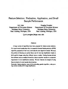
The test accuracies versus the sizes of feature subsets are illustrated in Fig. 2(A). From a feature selection context, we focus the comparison on the critical region as highlighted by a rectangle in this plot. In this region, the paired Wilcoxon signed-rank test was conducted to check whether a classifier significantly outperforms another one (see Fig. 2(B)). In addition to accuracy, the confusion matrices of different models, when selecting 16 features, are given in Fig. 2(C). First of all, with the comparison between our shallow DFS model and elastic net, it can be seen that our shallow model has a significantly higher test accuracy than elastic net for the same number of selected features. From a computational viewpoint, it hence corroborates that adding a sparse one-to-one layer is a better technique than the tradition of simply combining the feature subsets selected for each class. Second, from the comparison of our deep and shallow DFS models, it shows that a significantly better test accuracy can be obtained by our deep model. It hence supports that considering the non-linearity among the variables can contribute to the improvement of prediction capability. Third, it is interesting to see that random forest with certain top-ranked features performs better than the deep learning model. This may be because the structure and parameter of the deep model was not optimized. Finally, from the confusion matrices as shown in Fig. 2(C), we highlight that some active promoters tend to be classified as active enhancers. 0.90

p-value

Shallow DFS LASSO

Deep DFS 0.85

2.33e-4

Shallow DFS

8.30e-6

1.21e-2

5.96e-5

LASSO

1.32e-4

B Deep DFS

0.65

5

10 15 20 25 30 35 40 45 50 55 60 65 70 75 80 85 90 Number of Selected Features

A

LASSO A-E A-P BG

Predicted A-E A-P BG 587 75 56 63 641 15 50 50 619

Shallow DFS

Predicted A-E A-P BG 549 124 45 58 652 9 77 78 564

A-E A-P BG

Random Forest Actual

0.60 0

A-E A-P BG

Shee

Actual

0.70

Actual

Deep DFS Shallow DFS Elastic Net (alpha=1) Elastic Net (alpha=0.8) Elastic Net (alpha=0.5) Elastic Net (alpha=0.3) Elastic Net (alpha=0) Random Forest

Actual

Test Accuracy

0.80

0.75

Random Forest

9.82e-4

A-E A-P BG

Predicted A-E A-P BG 582 64 72 50 648 21 56 53 610 Predicted A-E A-P BG 622 50 46 59 640 20 45 34 640

C

Fig. 2: (A) The number of selected features by different methods and corresponding test accuracy. The critical region is highlighted by the orange rectangle. (B) p-value of the paired Wilcoxon signed-rank test in the critical region. (C) Confusion matrices when selecting 16 features by different models, respectively. A-E: Active Enhancer, A-P: Active Promoter, BG: Background.

We recorded the training times of the four models on the same computer. The shallow DFS, elastic net, and random forest took only 3.32, 6.56, and 2.68

Deep Feature Selection

9

seconds, respectively, to learn from data. However, the deep DFS model “unsurprisingly” consumed around 69.10 seconds. 3.3

Feature Analysis

We analyzed the features selected by the DFS models, LASSO, and random forest. We used a heatmap, as shown in Fig. 3, to visualize the regularization path in the sparse models. Since LASSO is supposed to have three (each for a class) heatmaps, we combined them by taking the corresponding maximal absolute values of its coefficients. That is, for a value of λ, we convert matrix W to a vector wnew by winew = max{|wi1 |, |wi2 |, |wi3 |}. First, we can see that the heatmaps of our shallow and deep DFS models are much sparser than that of LASSO. This implies that our scheme using a sparse one-to-one weighting layer is able to select a small subset of features along the regularization path, while LASSO tends to select more features, because it fuses all class-specific feature subsets. Second, comparing the result of the shallow DFS and LASSO, we can see many differences. For example, LASSO emphasizes CpG islands, TBLP1, and TBP, while they are not selected by the shallow DFS until later in the process. Instead, the heatmap of the shallow DFS indicates that ELF1, H2K27ac, Pol2, RUNX3, etc, are important features. From GeneCards [20] and literature, we surveyed the known functionality of features selected by the deep and shallow DFS in an early phase. The functionality and specificity of these features are given in Table 1, where the last column is our conclusion about the binding specificity of the features based on the box-plots (not given due to page limit) of our data. First, the table shows that deep DFS identifies more key features earlier than shallow DFS, such as BCL11A, HeK27me3, H3K4me1, H4K20me1, NRSF, TAF1, and TBP. Interestingly, the deep DFS found a non-linear relation: TAF1 and TBP are actually components of TFIID functioning as RNA polymerase II locator. Second, we can see that the known functionality of the majority of selected features, as highlighted in bold in Table 1 (i.e. ELF1, H3K27ac, Pol2, BATF, EBF1, H3K36me3, H3K4me2, NFYB, RUNX3, BCL11A, H3K27me3, H3K4me1, and NRSF), are consistent with the binding specificity drawn from our data. From the box-plots (not given) of our data, we are also able to identify novel enrichment of some features (emphasized by italic type in Table 1) in enhancers and inactive elements. For example, H3K9ac is thought to be enriched in actively transcribed promoters [12], our result show that it is also enriched in active enhancers. H4K20me1 is reported to be enriched in exons [25], our result also show that both inactive enhancers and inactive promoters are enriched with H4K20me1. TAF1 and TBP is known as a promoter binder, our result shows that they are also associated with active enhancers. Finally, it has to be mentioned that some cell-specific features can be identified by the DFS models. From Table 1, we can see that ELF1 [6], BATF [11], EBF1 [18], and BCL11A [14] are specific to lymphoid cells (recall that GM12878 is a lymphoblastoid cell line from blood). This thus further confirms that the selected features are highly informative.

Lambda

ATF2 ATF3 BATF BCL11A BCL3 BCLAF1 BHLHE40 BRCA1 CEBPB C−FOS(FOS) CHD1 C−MYC(MYC) COREST CPGISLANDS CTCF DNASE E2F4 EBF1 EGR1 ELF1 ELK1 ETS1 EZH2 FAIRE FOXM1 GABP(GABPA) GCN5 H2A.Z H3K27AC H3K27ME3 H3K36ME3 H3K4ME1 H3K4ME2 H3K4ME3 H3K79ME2 H3K9AC H3K9ME3 H4K20ME1 IKZF1 IRF3 IRF4 JUND MAX MAZ MEF2A MEF2C MTA3 MXI1 NFATC1 NFE2 NFIC NFKB NFYA NFYB NRF1 NRSF(REST) P300(EP300) PAX5 PBX3 PHASTCONS PML POL2(POLR2A) POL3(POLR3G) POU2F2 PU.1(SPI1) RAD21 RFX5 RUNX3 RXRA SIN3A SIX5 SMC3 SP1 SPT20(SUPT20H) SRF STAT1 STAT3 STAT5A TAF1 TBLR1(TBL1XR1) TBP TCF12 TCF3 TR4(NR2C2) USF1 USF2 WHIP(WRNIP1) YY1 ZBTB33 ZEB1 ZNF143 ZNF274 ZZZ3 −2 2

Feature

Value

Lambda

ATF2 ATF3 BATF BCL11A BCL3 BCLAF1 BHLHE40 BRCA1 CEBPB C−FOS(FOS) CHD1 C−MYC(MYC) COREST CPGISLANDS CTCF DNASE E2F4 EBF1 EGR1 ELF1 ELK1 ETS1 EZH2 FAIRE FOXM1 GABP(GABPA) GCN5 H2A.Z H3K27AC H3K27ME3 H3K36ME3 H3K4ME1 H3K4ME2 H3K4ME3 H3K79ME2 H3K9AC H3K9ME3 H4K20ME1 IKZF1 IRF3 IRF4 JUND MAX MAZ MEF2A MEF2C MTA3 MXI1 NFATC1 NFE2 NFIC NFKB NFYA NFYB NRF1 NRSF(REST) P300(EP300) PAX5 PBX3 PHASTCONS PML POL2(POLR2A) POL3(POLR3G) POU2F2 PU.1(SPI1) RAD21 RFX5 RUNX3 RXRA SIN3A SIX5 SMC3 SP1 SPT20(SUPT20H) SRF STAT1 STAT3 STAT5A TAF1 TBLR1(TBL1XR1) TBP TCF12 TCF3 TR4(NR2C2) USF1 USF2 WHIP(WRNIP1) YY1 ZBTB33 ZEB1 ZNF143 ZNF274 ZZZ3 −6 6

Feature

Value

H3K4ME1 POL2(POLR2A) TAF1 H3K4ME2 H3K27ME3 CPGISLANDS EBF1 TBP NRSF(REST) IKZF1 H3K79ME2 H3K27AC SRF BATF ZZZ3 H3K36ME3 RUNX3 BCL11A GCN5 H4K20ME1 H3K9AC PHASTCONS SIX5 SIN3A TR4(NR2C2) GABP(GABPA) SPT20(SUPT20H) NFIC BRCA1 ZNF274 NRF1 FAIRE MEF2A PML SP1 H2A.Z DNASE PU.1(SPI1) NFKB H3K4ME3 MXI1 SMC3 P300(EP300) STAT1 NFATC1 CTCF ELF1 CEBPB H3K9ME3 STAT3 MTA3 ATF2 E2F4 IRF4 ZBTB33 BHLHE40 IRF3 WHIP(WRNIP1) TBLR1(TBL1XR1) ETS1 BCL3 ATF3 C−MYC(MYC) EZH2 NFE2 TCF12 USF1 NFYB RXRA JUND TCF3 BCLAF1 PAX5 RAD21 POL3(POLR3G) RFX5 FOXM1 ZEB1 YY1 COREST C−FOS(FOS) NFYA MEF2C POU2F2 STAT5A MAZ USF2 ELK1 ZNF143 PBX3 MAX CHD1 EGR1

ATF2 ATF3 BATF BCL11A BCL3 BCLAF1 BHLHE40 BRCA1 CEBPB C−FOS(FOS) CHD1 C−MYC(MYC) COREST CPGISLANDS CTCF DNASE E2F4 EBF1 EGR1 ELF1 ELK1 ETS1 EZH2 FAIRE FOXM1 GABP(GABPA) GCN5 H2A.Z H3K27AC H3K27ME3 H3K36ME3 H3K4ME1 H3K4ME2 H3K4ME3 H3K79ME2 H3K9AC H3K9ME3 H4K20ME1 IKZF1 IRF3 IRF4 JUND MAX MAZ MEF2A MEF2C MTA3 MXI1 NFATC1 NFE2 NFIC NFKB NFYA NFYB NRF1 NRSF(REST) P300(EP300) PAX5 PBX3 PHASTCONS PML POL2(POLR2A) POL3(POLR3G) POU2F2 PU.1(SPI1) RAD21 RFX5 RUNX3 RXRA SIN3A SIX5 SMC3 SP1 SPT20(SUPT20H) SRF STAT1 STAT3 STAT5A TAF1 TBLR1(TBL1XR1) TBP TCF12 TCF3 TR4(NR2C2) USF1 USF2 WHIP(WRNIP1) YY1 ZBTB33 ZEB1 ZNF143 ZNF274 ZZZ3 −2 2

Feature

Value

Importance Lambda

(c) LASSO

14 12 10 8 6 4 2 0

Y. Li, C.-Y. Chen, and W.W. Wasserman 10

0.0282 0.0262 0.0242 0.0222 0.0202 0.0182 0.0162 0.0142 0.0122 0.0102 0.0082 0.0062 0.0042 0.0022 0.0002

(a) Deep DFS 0.0655 0.0605 0.0555 0.0505 0.0455 0.0405 0.0355 0.0305 0.0255 0.0205 0.0155 0.0105 0.0055 0.0005

(b) Shallow DFS 0.1247

0.0492

0.0194

0.0077

0.0030

0.0012

0.0005

0.0002

0.0001

Feature

(d) Random Forest

Fig. 3: Coefficients heatmaps of the DFS and LASSO models, and the importance of features ranked by random forest. In the heatmaps, as the value of λ decreases vertically down, more and more coefficient becomes nonzero. The strength of the colors indicates the involvement of features in classification. The higher a bar is, the earlier the corresponding feature affects the classification. Eventually, all features turn to nonzero, affecting the classification. A pink horizontal line in (a) is due to a failure of the stochastic gradient descent algorithm, which can be overcome by a different initial solution. In (d), the key features listed in Table 1 is coloured in red.

Deep Feature Selection

11

Table 1: Key features selected by the deep and shallow DFS models. The last column is the binding specificity of these features based on box-plots (not given) of our data. Features consistent between known functions and binding specificity are highlighted in boldface. Features having novel enrichment are emphasized in italic type. A: Active, I: Inactive, P: Promoter, E: Enhancer, Ex: Exon. Feature ELF1

Known Functions Specificity Primarily expressed in lymphoid cells. Bind to promoters A-P, A-E and enhancers [6]. Act as both activator and repressor. H3K27ac Enriched in the flanking regions of active enhancers and A-P, A-E active promoters [21]. Pol2 Encode RNA polymerase II to initialize transcription. A-P A-E BATF From AP-1/ATF superfamily. A negative regulator of AP-1/ATF transcriptional events. Interact with Jun family to recognize immune-specific regulatory element. Bind to enhancers [11]. EBF1 Bind to enhancers of PAX5 for B lineage commitment A-E [18]. H3K36me3 Enriched in transcribed gene body. A-E H3K4me2 Define TF binding regions [26]. P, A-E H3K9ac Enriched in transcribed promoters [12]. A-P, A-E NFIC Promoter binding transcription activator [19]. A-P, A-E NFYB Bind specifically to CCAAT motifs in the promoter reA-P gions. RUNX3 Serve as both activator and repressor. Bind to a core A-P, A-E DNA sequence of a number of enhancers and promoters. BCL11A Involved in lymphoma pathogenesis, leukemogenesis, and A-E, A-P hematopoiesis. Bind to promoters and enhancers [14]. H3K27me3 Enriched in closed or poised enhancers [21] and poised I-P, I-E promoters [27]. H3K4me1 Enriched in enhancer regions [21]. A-E H4K20me1 Enriched in exons [25]. A-Ex, I-P, I-E NRSF/RESTRepresses neuronal genes in non-neuronal tissues. With A-P corepressors, recruit histone deacetylase to the promoters of REST-regulated genes. TAF1 TAFs serve as coactivators. TAFs and TBP assemble A-P, A-E TFIID to position RNA polymerase II to initialize transcription. TBP TATA-binding Protein. Interact with TAFs. Bind to core A-P, A-E promoters.

Random forest is suitable for multi-class data. It can return the importance of each feature by measuring the decrease of out-of-bag error by permuting the values of this feature [7]. We compared the features selected by our models with the ones ranked by random forest, as shown in Fig. 3d. The majority of the key features selected by the DFS models are top-ranked in random forest, except that NFKB and ELF1 are scored as less important. It may be because

12

Y. Li, C.-Y. Chen, and W.W. Wasserman

our DFS model considers the dependency of the features, while random forest independently measures the impact of removing each feature from the model.

4

Conclusion

Linear methods do not model the non-linearity of variables and can not be extended to multi-class in a natural way for feature selection, while deep models learn non-linearity and high-level representation of features. In this paper, we propose the deep feature selection model for selecting input features in a deep structure, especially for multi-class data. We applied this model to distinguish active promoters and enhancers from the rest of the genome. Our result shows that our shallow and deep DFS models are able to select a smaller subset of features than LASSO with comparable accuracy. Furthermore, our deep DFS can select discriminative features that may be overlooked by the shallow DFS. Through looking into the genomic features selected, we find that the features selected by DFS are biological plausible. Furthermore, some selected features have novel enrichment in regulatory elements. In future work, we will evaluate the new model on simulated data in order to further understand its behaviour. New sparse regulators and efficient model selection methods will be investigated to improve the performance of our model. Acknowledgments. Dr. Anthony Mathelier (UBC) and Wenqiang Shi (UBC) provided valued suggestions. Dr. Anshul Kundaje (Stanford) provided valuable instruction during the processing of ChIP-seq data from ENCODE.

References 1. Ackley, D., Hinton, G., Sejnowski, T.: A learning algorithm for Boltzmann machines. Cognitive Science pp. 147–169 (1985) 2. Andersson, R., Gebhard, C., Miguel-Escalada, I., et al.: An atlas of active enhancers across human cell types and tissues. Nature 507, 455–461 (2014) 3. Bengio, Y., Courville, A., Vincent, P.: Representation learning: A review and new perspectives. IEEE Transactions on Pattern Analysis and Machine Intelligence 35(8), 1798–1828 (2013) 4. Bergstra, J., Breuleux, O., Bastien, F., Lamblin, P., Pascanu, R., Desjardins, G., Turian, J., Warde-Farley, D., Bengio, Y.: Theano: a CPU and GPU math expression compiler. In: The Python for Scientific Computing Conference (SciPy) (Jun 2010) 5. Bradley, P., Mangasarian, O.: Feature selection via concave minimization and support vector machines. In: International Conference on Machine Learning. pp. 82–90. Morgan Kaufmann Publishers Inc. (1998) 6. Bredemeier-Ernst, I., Nordheim, A., Janknecht, R.: Transcriptional activity and constitutive nuclear localization of the ETS protein Elf-1. FEBS Letters 408(1), 47–51 (1997) 7. Breiman, L.: Random Forests. Machine learning 45, 5–32 (2001) 8. Friedman, J., Hastie, T., Tibshirani, R.: Regularization paths for generalized linear models via coordinate descent. Journal of Statistical Software 33, 1–22 (2010)

Deep Feature Selection

13

9. Hinton, G., Salakhutdinov, R.: Reducing the dimensionality of data with neural networks. Science 313, 504–507 (2006) 10. Hinton, G., Osindero, S., Teh, Y.: A fast learning algorithm for deep belief nets. Neural Computation 18, 1527–1554 (2006) 11. Ise, W., Kohyama, M., Schraml, B., Zhang, T., Schwer, B., Basu, U., Alt, F., Tang, J., Oltz, E., Murphy, T., Murphy, K.: The transcription factor BATF controls the global regulators of class-switch recombination in both B cells and T cells. Nature Immunology 12(6), 536–543 (2011) 12. Kratz, A., Arner, E., Saito, R., Kubosaki, A., Kawai, J., Suzuki, H., Carninci, P., Arakawa, T., Tomita, M., Hayashizaki, Y., Daub, C.: Core promoter structure and genomic context reflect histone 3 lysine 9 acetylation patterns. BMC Genomics 11, 257 (2010) 13. LeCun, Y., Bottou, L., Bengio, Y., Haffner, P.: Gradient-based learning applied to document recognition. Proceedings of the IEEE 86(11), 2278–2324 (1998) 14. Lee, B., Dekker, J., Lee, B., Iyer, V., Sleckman, B., Shaffer, A.I., Ippolito, G., Tucker, P.: The BCL11A transcription factor directly activates rag gene expression and V(D)J recombination. Molecular Cell Biology 33(9), 1768–1781 (2013) 15. Li, Y.: Deep learning package, https://github.com/yifeng-li/deep_learning 16. Li, Y., Ngom, A.: Classification approach based on non-negative least squares. Neurocomputing 118, 41–57 (2013) 17. LISA Lab: Deep learning tutorials, http://deeplearning.net/tutorial 18. Nechanitzky, R., Akbas, D., Scherer, S., Gyory, I., Hoyler, T., Ramamoorthy, S., Diefenbach, A., Grosschedl, R.: Transcription factor EBF1 is essential for the maintenance of B cell identity and prevention of alternative fates in committed cells. Nature Immunology 14(8), 867–875 (2013) 19. Pjanic, M., Pjanic, P., Schmid, C., Ambrosini, G., Gaussin, A., Plasari, G., Mazza, C., Bucher, P., Mermod, N.: Nuclear factor I revealed as family of promoter binding transcription activators. BMC Genomics 12, 181 (2011) 20. Rebhan, M., Chalifa-Caspi, V., Prilusky, J., Lancet, D.: Genecards: Integrating information about genes, proteins and diseases. Trends in Genetics 13(4), 163 (1997) 21. Shlyueva, D., Stampfel, G., Stark, A.: Transcriptional enhancers: From properties to genome-wide predictions. Nature Review Genetics 15, 272–286 (2014) 22. The ENCODE Project Consortium: An integrated encyclopedia of DNA elements in the human genome. Nature 489, 57–74 (2012) 23. The FANTOM Consortium, The RIKEN PMI, CLST (DGT): A promoter-level mammalian expression atlas. Nature 507, 462–470 (2014) 24. Tibshirani, R.: Regression shrinkage and selection via the Lasso. Journal of the Royal Statistical Society. Series B (Methodological) 58(1), 267–288 (1996) 25. Vakoc, C., Sachdeva, M., Wang, H., , Blobel, G.: Profile of histone lysine methylation across transcribed mammalian chromatin. Molecular and Cellular Biology 26(24), 9185–9195 (2006) 26. Wang, Y., Li, X., Hua, H.: H3K4me2 reliably defines transcription factor binding regions in different cells. Genomics 103(2-3), 222–228 (2014) 27. Zhou, V., Goren, A., Bernstein, B.: Charting histone modifications and the functional organization of mammalian genomes. Nature Review Genetics 12, 7–18 (2011) 28. Zou, H., Hastie, T.: Regularization and variable selection via the elastic net. J. R. Stat. Soc. Series B Stat. Methodol. 67(2), 301–320 (2005)