Junsik Kim and Takeo Kanade, “Degeneracy of the Linear Seventeen-Point Algorithm for Generalized Essential Matrix,” Journal of Mathematical Imaging and Vision, Vol. 37, No. 1, May 2010, pp. 40-48. J Math Imaging Vis (2010) 37: 40-48 DOI 10.1007/s10851-010-0191-9 Authors’s version. The final publication is available at www.springerlink.com.
Degeneracy of the Linear Seventeen-Point Algorithm for Generalized Essential Matrix Jun-Sik Kim · Takeo Kanade
c °Springer Science+Business Media, LLC 2010
Abstract In estimating motions of multi-centered optical systems using the generalized camera model, one can use the linear seventeen-point algorithm for obtaining a generalized essential matrix, the counterpart of the eight-point algorithm for the essential matrix of a pair of cameras. Like the eight-point algorithm, the seventeen-point algorithm has degenerate cases. However, mechanisms of the degeneracy of this algorithm have not been investigated. We propose a method to find degenerate cases of the algorithm by decomposing a measurement matrix that is used in the algorithm into two matrices about ray directions and centers of projections. This decomposition method allows us not only to prove degeneracy of the previously known degenerate cases, but also to find a new degenerate configuration. Keywords Motion Estimation · Generalized Essential Matrix · Degenerate Case · Matrix Decomposition · Rank Deficiency · Null space 1 Introduction Non-conventional optical imaging, such as an omnidirectional mirror system and a multiple-camera system, has been used in a wide range of computer vision applications [2, 4–6, 11]. One benefit of using such optical systems is to have a wider field of view, which reduces ambiguities between translation and rotation in estimating motions of the cameras [1]. Jun-Sik Kim · Takeo Kanade Robotics Institute, Carnegie Mellon University, 5000 Forbes Avenue, Pittsburgh, PA, 15213, USA Tel.: +1-412-268-5622 E-mail:
[email protected] Takeo Kanade E-mail:
[email protected]
Image formation or projection models of these systems, not describable by a conventional pin-hole camera model, is nonlinear, each different from others depending on the mirror and camera configurations. The classical linear epipolar constraint for the pin-hole model is not applicable here, and thus the motion estimation between frames becomes a highly nonlinear problem. To deal with non-conventional imaging, a general model of cameras has been proposed by regarding any optical system as a set of multi-centered linear projections [6]. In this generalized camera model, an epipolar constraint can be expressed in a linear form [10], which has resulted in the seventeen-point linear algorithm for motion estimation. The 17-point algorithm has degenerate cases. Sturm [14] first gives a list of the degenerate cases together with the corresponding generalized essential matrices. However, the paper does not provide the reason why those cases are degenerate, or whether there are other degenerate cases of the algorithm. Later, Mouragnon et al. [9] and Li et al. [8] give analysis about the degenerate cases and the ranks of the measurement matrices. In both papers, they show the degeneracy on the given specific cases which have been verified by example. In this paper, we aim to find the complete set of degenerate configurations by deduction, not by examples. We show that by decomposing a measurement matrix of the 17-point algorithm, we can systematically identify degeneracy of the algorithm, revealing the reasons of how the degeneracy occurs. 2 Epipolar Constraint of Generalized Cameras We derive a linear constraint that exists between a pair of corresponding points in two frames taken by a mov-
2
J Math Imaging Vis (2010) 37: 40-48
ing generalized camera, similar to the classical epipolar constraint in the case of a projective camera [10, 14]. 2.1 Generalized Camera
where [ ]× denotes a skew-symmetric matrix of a vector [10, 14]. Note the similarities of this form (4) to the epipolar constraint of pin-hole cameras [7]. First, the upperleft submatrix of the matrix is − [t]× R, which is the same form with an essential matrix of a projective camera. Second, Eq. (4) is a bilinear form on Pl¨ ucker coordinates, as the epipolar constraints of pin-hole cameras is on image coordinates. To emphasize these similarities, we can define Eg by using the essential matrix E of the epipolar constraint of a projective camera.
One method to describe image formation of a multicentered imaging system is to assign a 3D ray of light to each pixel. Because determining the 3D ray is not based on the optical model of the imaging system, this generalized camera model can be used for an arbitrary optical system. E , [t]× R To represent a light ray in the 3D space, a Pl¨ ucker ¸ · coordinate is used. This representation uses two 3-vectors: −E R 0 Eg , . a direction vector q and a moment vector q defined as R 03×3 q0 = q × O
(1)
where O is an arbitrary point on the ray, for which in our case, the projection center can be conveniently selected. Obviously, the relation q> q0 = 0 holds, and thus Pl¨ ucker coordinates are defined up to scale. Calibration of a generalized camera is to map a 3D ray to each pixel, for which Ramalingam et al. [12] present a method. In this paper, we assume a calibrated generalized camera as in the previous work [10, 14]. 2.2 Generalized Essential Matrix We are now ready to derive the epipolar constraint for multi-centered optical systems by using the generalized camera model [1]. Suppose that a calibrated generalized camera moves with rotation R and translation t, and that we have a pair of 3D ray correspondences < q1 , q01 > and < q2 , q02 >. The first 3D ray < q1 , q01 > is transformed due to the camera motion into < Rq1 , Rq01 − (t × R) q1 > .
(2)
This should intersect with < q2 , q02 >, which generates the following constraint1 . >
q2 > (Rq01 − (t × R) q1 ) + q02 Rq1 = 0. This constraint equation is rewritten as >
0 q2 > Rq1 0 − q> 2 [t]× Rq1 + q2 Rq1 = 0,
or in a matrix form, · ¸> · ¸· ¸ − [t]× R R q2 q1 = 0, q02 q01 R 03×3 1
(3)
(4)
In the Pl¨ ucker coordinate representation, if two rays < m1 , m01 > and < m2 , m02 > intersect, they satisfy m1 > m02 + m01 > m2 = 0.
(5) (6)
The matrix Eg is called a generalized essential matrix, and Eq. (3) or (4) is known as a generalized epipolar constraint for given measurements < q1 , q01 > and < q2 , q02 >. 3 Seventeen-point Algorithm for Generalized Essential Matrix The generalized essential matrix Eg depends on the motion parameters R and t, and it has only 6 degrees of freedom (DOF). However, 6-DOF parameterization of Eg is so nonlinear that it is hard to find the parameters from 3D-ray correspondences. The simplest solution is to make it linear by increasing the number of unknowns, as in the 8-point algorithm for a projective essential matrix. The matrix Eg has two unknown matrices E and R. If we assume as if all of the 18 elements of the two matrices are independent, Eq. (4) becomes a linear equation as · ¸ > e =0 (7) a (q1 , q01 , q2 , q02 ) r where a (q1 , q01 , q2 , q02 ) is a measurement vector from the corresponding rays, and 9-vectors e and r are vectorized E and R, respectively. Because this constraint equation (7) is defined up to scale, this system has 17 DOFs in total. The minimum number of correspondences required for a solution is 17, because one pair of correspondences gives one constraint equation. By stacking the measurement vectors a (q1 , q01 , q2 , q02 ) of n correspondences, one can build a measurement matrix A as ´ ³ 1 1 a q11 , q01 , q12 , q02 ´ ³ a q2 , q0 2 , q2 , q0 2 1 1 2 2 A= (8) .. . ¡ n n¢ a qn1 , q01 , qn2 , q02
J Math Imaging Vis (2010) 37: 40-48
X2 X1
3 >
X3
¢¢¢
q2 = [q2x q2y q2z ] , the 9-vector aE (q1 , q2 ) is a vectorized q2 q> 1 expressed as
Xn
aE (q1 , q2 )9×1 = [q1x q2x q1x q2y q1x q2z ...
O 002 O001
O02
q1y q2x q1y q2y q1y q2z ...
O000 2
q1z q2x q1z q2y q1z q2z ]
O01
O000 1 Fig. 1 Motion of a multi-camera system. The center O1 is transformed to O2 by a rigid body motion R and t. Note that the superscript in the text refers to an index of corresponding rays. For example, the centers O21 and O22 of the corresponding rays for the point X2 in the text are O01 and O00 2 in this case, respectively.
where superscripts denote the indices of the corresponding rays. In general, the one-dimensional null space of A to be found by singular value decomposition is a solution for e and r defined up to scale. The scale can be determined by adjusting the norm of the estimated rotation matrix R to be one. As in the 8-point algorithm, once e and r are determined in this way, one can use them as the initial estimates to obtain the improved solution of Eg by solving the nonlinear equations. The degeneracy of the 17-point algorithm occurs when the null space of A has two or more dimensions, and thus the solution is not unique. In the next section, we will derive the conditions of the measurement matrix A that causes such degeneracy.
Similarly, we will obtain the form of aR . By using > 0 (1), the term q02 Rq1 +q> 2 Rq1 in Eq. (3) can be rewritten as q2 > ([O2 ]× R − R[O1 ]× ) q1
(11)
where O1 and O2 are the centers of the corresponding rays < q1 , q01 > and < q2 , q02 >, respectively. Note that, just like q> 2 Eq1 , term (11) is also a bilinear form of q1 and q2 as a whole. Thus, (11) can be rewritten in the form of > aE (q1 , q2 ) v(R, O1 , O2 ) where v(R, O1 , O2 ) is a vectorized [O2 ]× R − R[O1 ]× , which is a linear combination of r. Therefore, a> R in Eq. > (9) should be a linear transformation of aE (q1 , q2 ) to be expressed as >
a> R = aE (q1 , q2 ) C (O1 , O2 )
(12)
where C (O1 , O2 ) is a 9 × 9 block-structured matrix:
[O2 ]× C (O1 , O2 ) = O1z I3×3 −O1y I3×3
−O1z I3×3 [O2 ]× O1x I3×3
O1y I3×3 −O1x I3×3 [O2 ]× (13)
4 Mechanisms of Degeneracy of Seventeen-Point Algorithm
>
To study the degeneracy, we will first show that the matrix A is decomposable into two matrices: one about the direction vectors of rays and the other about the projection centers. Then, we can study how the degeneracy can occur by looking into only the second matrix. Fig.1 shows the motion of a multi-camera system and the transformation of camera centers O1 and O2 . 4.1 Decomposition of Measurement Matrix A Eq. (7) can be rewritten in the form > a> E e + aR r = 0.
(10)
>
(9)
where the measurement 18-vector a (q1 , q01 , q2 , q02 ) is divided into the two 9-vectors aE and aR . From q> 2 Eq1 in (3) and (5), we see that aE is dependent only on > q1 and q2 , and if we denote q1 = [q1x q1y q1z ] and
>
and O1 = [O1x O1y O1z ] , O2 = [O2x O2y O2z ] . As the matrix C (O1 , O2 ) depends only on the projection centers O1 and O2 , we call it a center matrix. It is skew-symmetric; it is a sum of a block-diagonal matrix of skew-symmetric matrices, and a block-skewsymmetric matrix of three diagonal matrices. According to Jacobi’s theorem2 [3], therefore, this center matrix (13) should be rank-deficient. By using the center matrix, Eq. (7) is now rewritten as · ¸ ¤ e >£ aE (q1 , q2 ) I9×9 C (O1 , O2 ) = 0. (14) r 2 Any skew-symmetric matrix of odd order has determinant equal to 0.
4
J Math Imaging Vis (2010) 37: 40-48
The measurement matrix A is therefore decomposed into two matrices Ad and Ac . > ¢ > ¡ a1E a1E C O11 , O12 2 > 2 > ¡ 2 2 ¢ aE aE C O1 , O2 A= .. .. . . n> n> n n aE aE C (O1 , O2 ) > ¡ ¢ a1E 0 ··· 0 I9×9 C ¡O11 , O12 ¢ I9×9 C O21 , O22 0 a2E > · · · 0 = . .. .. .. . . .. . . .. . . . n n n> I C (O , O ) 9×9 0 0 · · · aE 1 2 9n×18 n×9n
, Ad Ac (15) where superscripts denote the indices of the corresponding rays, as in (8). The first n × 9n matrix Ad depends only on the ray directions, and the second 9n × 18 matrix Ac on the positions of projection centers. Because the ray directions can be different on the different scene features, we are interested in the degenerate cases relating only on the Ac , which gives information about the configurations of a generalized camera.
For each case, the null space of the center matrix is found as follows. Proposition 2 If |O1 | 6= |O2 |, the null space of the center matrix C(O1 , O2 ) is £ ¤ > > > O1x O> 2 O1y O2 O1z O2
(17)
which is the vectorized rank-1 matrix O2 O> 1.
(18)
Proof This is proved by substituting O2 O> 1 for X in the original equation (16). u t Proposition 3 If |O1 | = |O2 |, a vector in the 3-D null space of the rank−6 center matrix is expressed in the matrix form with scalars a, b and θ as ¡ ¢ ¯ 1 ) + bO ¯ 1O ¯> RO aR(θ; O (19) 1 where RO is a rotation which satisfies O2 = RO O1 , ¯ 1 , O1 /|O1 |. R(θ; O ¯ 1 ) represents a rotation around and O ¯ 1 by angle θ. the axis O If O1 = O2 , the null space includes I3×3 in a matrix form.
4.2 Null Space of the Center Matrix C(O1 , O2 ) The null space of a center matrix plays a key role in the remainder of this paper, so we will investigate the nullity and the null space of a center matrix. Finding the null space of the center matrix C(O1 , O2 ) is equivalent to solving the equation [O2 ]× X − X[O1 ]× = 03×3 ,
three eigenvalues are common. Therefore, the nullity of the center matrix is three and the rank is 6. u t
(16)
Proof Since |O1 | = |O2 |, O1 can be appropriately rotated to O2 , i.e., O2 = RO O1 . By adopting this rotation matrix, Eq. (16) becomes [RO O1 ]× X − X[O1 ]× = 03×3 .
(20)
One can see the three matrices RO , RO O1 O> 1 , and RO [O1 ]×
which is a Sylvester equation AX + XB = C [13] with C = 03×3 . Because the dimension of the solution space of the equation AX + XB = 0 is the same with the number of the common eigenvalues of A and B, we can prove the following proposition.
satisfy Eq. (20). By Gram-Schmidt orthogonalization, we can construct these orthogonal bases as ¡ ¢ ¯ 1 ]× , RO I3×3 − O ¯ 1O ¯ > and RO O ¯ 1O ¯> RO [O 1 1
Proposition 1 If |O1 | 6= |O2 |, that is, the lengths of the vector O1 and the vector O2 are not the same, the nullity of the center matrix is one; its rank is eight. Otherwise, the nullity becomes three; its rank is six.
¯ 1 , O1 /|O1 |. A vector in the where the unit vector O null space of a rank-6 center matrix is expressed in the matrix form using the orthogonal bases as ¡ ¡ ¢ ¢ ¯ 1O ¯ > + γO ¯ 1O ¯> RO α[O¯1 ]× + β I3×3 − O 1
Proof The skew-symmetric matrix [O1 ]× has the three eigenvalues: zero, and two imaginary values, 0, i|O1 | and − i|O1 |. Therefore, if |O1 | 6= |O2 |, [O1 ]× and [O2 ]× have one common eigenvalue, and the null space of the center matrix is one-dimensional. Thus, the rank of the 9 × 9 center matrix is 8. Otherwise, i.e. |O1 | = |O2 |, all the
1
with scalars α, β and γ. By using the fact that a rotation by angle θ around the unit axis vector u is expressed in general as R(θ; u) = sin θ[u]× + cos θ(I3×3 − uu> ) + uu> , this 3-D null space can be written in the form of ¡ ¢ ¯ 1 ) + bO ¯ 1O ¯> RO aR(θ; O 1
with scalars a, b, and θ. u t
J Math Imaging Vis (2010) 37: 40-48
4.3 Rank Analysis of the Measurement Matrix A We have shown that the measurement matrix A of the 17-point algorithm can be decomposed as A = Ad Ac . Using the decomposition, we can show the following propositions. Proposition 4 The rank of the measurement matrix A is invariant to the selection of coordinate systems of a generalized camera. Proof A measurement matrix A is constructed from a set of corresponding rays. Suppose that the rays are represented in different coordinate systems: coordinate of the system before the motion is transformed by {R1 , t1 }, and that after the motion by {R2 , t2 }. The directions and centers of the rays in the new coordinates are represented ˆ ˆ 1 = R> q 1 q1 and O1 = R1 O1 + t1 ˆ ˆ 2 = R> q 2 q2 and O2 = R2 O2 + t2 . In these different coordinate systems, another measureˆ is constructed as ment matrix A 1> 1> ˆE a ˆR a .. .. . ˆ A= . (21) . n> ˆ n> ˆR a E a
The vector aE for A is a vectorized q2 q> 1 in (10). > ˆ ˆ ˆ ˆ The vector aE for A is a vectorized q2 q1 which is equal > ˆE should be a linear combinato R> 2 q2 q1 R1 . Thus, a tion of aE as > ˆ> a E = aE T(R1 , R2 ).
where T(R1 , R2 ) is a 9×9 transformation matrix equal to R1 ⊗ R2 , which is the Kronecker product of R1 and R2 . ˆR is derived from (11), Similarly, a
5
Proposition 5 If Ac has a null space, the 17-point algorithm is degenerate. Proof Assume that the 17-point algorithm is not degenerate, that is, the nullity of the matrix A is only one. We will show that this assumption will lead to that the nullity of Ac is zero. Because A = Ad Ac , the null space of Ac , if exists, should be in the null space of A. The nullity of A should be greater than or equal to the nullity of Ac . Therefore, since the nullity of A is assumed to be one, the nullity of Ac should be one or zero. Assume that the nullity of Ac is one, then its null space should be the same as A. Let {E0 , R0 } denote the unique solution of the 17-point algorithm and e0 and r0 are vectorized E0 and R0 , respectively. From the definition of Ac in Eq. (15), ¢ ¡ e0 + C Oi1 , Oi2 r0 = 0 (23) for all i. Thus, for all i and j, r0 should satisfy ³ ´ ¡ ¢ C Oi1 , Oi2 r0 = C Oj1 , Oj2 r0 .
(24)
This be in the null space of ´ ³ means that r0 should j j i i C O1 − O1 , O2 − O2 . Let us divide the cases depending on the lengths of Oi1 − Oj1 and Oi2 − Oj2 . If |Oi1 − Oj1 | 6= |Oi2 − Oj2 | for some i and j, the ´> ´³ ³ matrix form of r0 , R0 = Oi2 − Oj2 Oi1 − Oj1 , and its rank is one from Proposition 2. Because the rank of a valid rotation matrix R0 should be three, the assumed solution {E0 , R0 } can not be a legitimate solution of the 17-point algorithm. If |Oi1 − Oj1 | = |Oi2 − Oj2 | for all i and j, the valid rotation R0 should satisfy that (Oi2 − Oj2 ) = R0 (Oi1 − Oj1 )
for all i and j, from Proposition 3. This is satisfied if and only if there exist a 3-vector ∆O such as Oi2 = ˆ 2 ]× R ˆ − R[ ˆ O ˆ 1 ]× )ˆ ˆ> q ([ O q 1 2 R0 Oi1 + ∆O for all i. According to the Proposition 4, > ˆ ˆ = q> R ([R O + t ] R − R[R O + t ] )R q the rank of this measurement matrix is equal to that 2 2 2 2 × 1 1 1 × 2 1 1 © ª > > of the measurement matrix in case that Oi1 = Oi2 for = q> [O ] R − R[O ] + [R t ] R − R[R t ] q 2 × 1 × 1 2 2 2 × 1 1 × all i. Because C(Oi1 , Oi1 ) has a vectorized I3×3 as a > ˆ common null space, from Proposition 3, the nullity of ˆ R is expressed where R = R2 RR1 . Thus, the vector a ˆ c is greater than one. This shows that the measureA as ment matrix A has two or more dimensional null space, ˆ> a R = which contradicts the assumption. © ª > aE (q1 , q2 )> C(O1 , O2 ) + C(R> t , R t ) T(R , R ). In total, if the measurement matrix A has an one1 2 1 2 1 2 dimensional null space, the nullity of Ac should be zero. ˆ is expressed as Eq. (22). The measurement matrix A Inversely, if Ac is rank-deficient, the solution can not Because the 18×18 matrix M is full-rank, the rank of be uniquely determined. t u ˆ is same with that of A. t A u
6
J Math Imaging Vis (2010) 37: 40-48
1> ¡ ¢ ¡ ¢ > > aE T(R1 , R2 ) a1E {C O11 , O12 + C R> 1 t1 , R2 t2 }T(R1 , R2 ) a2 > T(R , R ) a2 > {C ¡O2 , O2 ¢ + C ¡R> t , R> t ¢}T(R , R ) 1 2 1 2 1 2 1 1 2 2 E ˆ = E A .. .. . . ¡ n n¢ ¡ > ¢ > > n n > aE T(R1 , R2 ) aE {C O1 , O2 + C R1 t1 , R2 t2 }T(R1 , R2 ) ¡ ¢ · ¸ > T(R1 , R2 ) C R> 1 t1 , R2 t2 T(R1 , R2 ) , AM. = Ad Ac 0 T(R1 , R2 )
Proposition 6 If all the center matrices have a common null space, Ac has its null space. Inversely, if Ac has its null space, it is always possible to select the appropriate camera coordinate system such that all the center matrices have a common null space. Proof (⇒) If all the center matrices in Ac have a com£ ¤ > > mon null space N, the vector 0> should be a 9 N non-zero null vector of Ac from the form of (15). (⇐) Assume that the one-dimensional null space of Ac is composed with two 9-vectors x1 and x2 . Thus, for all i, x1 and x2 satisfy ¡ ¢ x1 + C Oi1 , Oi2 x2 = 09×1 (25) According to Proposition 4, changing the camera coorˆ = AM, and the center matrix C ˆ dinate system gives A in the newly selected coordinate system is represented by ¡ ¢ ˆ Oi , Oi = C 1 2 ¡ ¡ ¢ ¡ ¢¢ > T(R1 , R2 )−1 C Oi1 , Oi2 + C R> T(R1 , R2 ) 1 t1 , R2 t2 ˆ 2 = T(R1 , R2 )−1 x2 . Thus, and the vector x ¡ ¢ ˆ Oi , Oi x C 1 2 ˆ2 = ¢¢ ¢ ¡ ¡ ¡ > x2 . T(R1 , R2 )−1 C Oi1 , Oi2 + C R> 1 t1 , R2 t2 From Eq. (25), these center matrices have the common exists ¢ a matrix ¡ null space ¢ if and only ¡if there > > > t such that C R t , R t t , R C R> 1 1 2 2 x2 − x1 = 2 2 1 1 09×1 . We can always find the matrix that satisfies this condition by selecting R1 = R2 = I3×3 , t1 = −Oi1 and t2 = −Oi2 for any i. t u This proposition shows that we can find the degeneracy by checking only whether all the center matrices of the corresponding rays have a common null space. 5 Various Degenerate Configurations of Seventeen-point Algorithm We have shown that if all the center matrices have a common null space, the 17-point algorithm is degenerate: it can not have a unique solution. We identify those degenerate cases by investigating the center matrices.
(22)
To identify the degeneracy, we categorize the configurations into three cases with the rank of the center matrices as follows. 1. The rank of the center matrix is 8 for all the corresponding rays i. 2. The rank of the center matrix is less than 8 for all the corresponding rays i. 3. The rank of the center matrix is 8 for some corresponding rays i. Note that all the configurations relating to the projection centers are in these three categories, and thus, the analysis here gives the complete list of the degenerate cases about the camera configurations. 5.1 Case 1: The rank of the center matrix is 8 for all the corresponding rays. We have shown in Proposition 2 that if |Oi1 | 6= |Oi2 |, the rank of the 9 × 9 center matrix C(Oi1 , Oi2 ) is 8 and its null space has a form of (17) in a 9-vector or a form of (18) in a matrix form. All the center matrices of corresponding rays have a common null space, if and only if, for each pair of corresponding rays i, there exists a scalar ki to satisfy that i i> O12 O1> 1 = ki O2 O1 .
(26)
This condition is satisfied if and only if there exist scalars ki1 and ki2 for each i such that Oi1 = ki1 O11 and Oi2 = ki2 O12 .
(27)
Eq. (27) means that all the projection centers Oi1 before the motion are on a line, and all the centers Oi2 are aligned on a line after the motion. The 17-point algorithm becomes degenerate, if all the rays pass through a line before and after the motion of the rig. Fig. 2(a) illustrates this degenerate case. 5.2 Case 2: The rank of the center matrix is less than 8 for all the corresponding rays. We have shown in Proposition 1 that the rank of the center matrix C(Oi1 , Oi2 ) is less than 8 if and only if
J Math Imaging Vis (2010) 37: 40-48
7
|Oi1 | = |Oi2 |; in other words, there is a rotation matrix RiO that rotates Oi1 to Oi2 such that Oi2 = RiO Oi1 . From Proposition 3, the null space Ni of the center matrix of the corresponding rays i is expressed as ¢ ¡ ¯ i ) + bi O ¯iO ¯ i> (28) Ni = RiO ai R(θi ; O 1 1 1
Case 2-3: ai 6= 0 and bi = 0. Eq. (30) becomes a form of a Sylvester equation,
¯ i = Oi /|Oi |. There is the common null space where O 1 1 1 of the two center matrices of corresponding rays i and j, if and only if the null space Ni is a solution of the original Sylvester equation of the ray j, that is,
¯ i )> Ri> Rj R(θj ; O ¯ j ) = I3×3 , R(θi ; O 1 O 1 O
¯ j ]× Ni = Ni [O ¯ j ]× . [RjO O 1 1
(29)
By substituting (28), separating terms that include ai and bi into the left and the right sides, respectively, ¯ i )> Ri> Rj from the left, this and multiplying R(θi ; O 1 O O becomes ³ ´ ¯ i )> Ri> Rj O ¯j ¯j ai [R(θi ; O 1 O O 1 ]× − [O1 ]× = ´ ³ ¯ i )> [Ri> Rj O ¯ j ]× O ¯iO ¯ i> − O ¯iO ¯ i> [O ¯ j ]× . − bi R(θi ; O 1 O 1 1 1 1 1 O 1 (30) The left-hand side of Eq. (30) is skew-symmetric, but the right-hand side is not. Therefore, this equation can hold if and only if the both sides are 0-matrices. Let us divide the possible conditions into four subcases based on ai and bi . Case 2-1: ai = bi = 0. The null space Ni becomes zero, which is a trivial solution. Case 2-2: ai = 0 and bi 6= 0. Eq. (30) becomes a form of a Sylvester equation, j ¯j ¯ i ¯ i> ¯ i ¯ i> ¯ j [Ri> O RO O1 ]× O1 O1 − O1 O1 [O1 ]× = 0.
¯iO ¯ i> From Proposition 3, we obtain a condition O 1 1 = i> j ¯ j ¯ j> RO RO O1 O1 as its rank-1 solution, and further from the definition of RiO and RjO , it becomes ¯ i = ±O ¯ j and O ¯ i = ±O ¯ j. O 1 2 1 2
(31)
¯ i = Oi /|Oi |, these conditions become Eq. Because O 1 1 1 (27), which means that all the projection centers Oi1 before the motion are on a line, and all the centers Oi2 after the motion are also aligned on a line, as in Section 5.1. As a subcase of (31), if the conditions are Oi1 = O1 and Oi2 = O2 , that is, if all the rays pass through one point in each time step (as shown in Fig. 2(b)), it means that, in practice, a single pinhole camera or an optical mirror system having a single focal point is degenerate.
¯ i )> Ri> Rj O ¯j ¯j [R(θi ; O 1 O O 1 ]× − [O1 ]× = 0. From Proposition 3, we can find a condition
or ¯ i ) = Rj R(θj ; O ¯ j) RiO R(θi ; O 1 1 O
(32)
¯ i )Oi , Eq. (32) shows that there Because Oi1 = R(θi ; O 1 1 exists a common rotation Rc for all i such that Oi2 = Rc Oi1 .
(33)
By rotating the center Oi2 to Oi1 using a common rotation Rc , the center matrix C(Oi1 , Oi2 ) becomes C(Oi1 , Oi1 ), whose null space includes a vectorized I3×3 common to i. Therefore, if each corresponding ray pair passes through the same point in the local coordinate system before and after the motion, as shown in Fig. 2(c), the 17-point algorithm becomes degenerate regardless of the positions of the centers. This situation usually occurs when using multiple cameras with nonoverlapping FOVs in which case correspondences are often tracked only between frames in the same cameras, thus causing the 17-point algorithm to be degenerate. Case 2-4: ai 6= 0 and bi 6= 0. In this case, the both (31) and (32) should be satisfied. Thus, physically, all the camera centers are aligned on a line before and after the motion, respectively, and the corresponding rays should pass through the same point in the local coordinate before and after the motion. Fig. 2(d) shows this degeneracy. Although the null space of a center matrix is 3dimensional in (28), the degeneracy occurs only dependent on the values of ai and bi , not on θi . This is because the term θi is a parameter of a rotation matrix whose axis is the direction to the center position. As in deriving (33), the rotation matrix does not change the coordinate of the centers at all, and does not affect the degeneracy. 5.3 Case 3: The rank of the center matrix is 8 for some corresponding rays, but not all. With the two previous cases, we have investigated when rank(C(Oi1 , Oi2 )) = 8 for all i, and when rank(C(Oi1 , Oi2 )) < 8 for all i. The only remaining case is that rank(C(Oi1 , Oi2 )) = 8 for some i. In this case, there are two sets of center matrices: one of the rank-8 matrices, and the other of the rank 1 . This should be a solution of the Sylvester equation of the rank RO O1 × O2 O> 1 − O2 O1 O1 × = 0. Thus, there should be a scalar ki for all i such that i i i O2 O> 1 = ki RO O1 O1
>
= ki Oi2 Oi> 1 .
This is the same with Eq. (26) in Case 1. Thus, if all the centers are aligned on a line before and after the motion respectively as in Case 1, the 17-point algorithm is degenerate. 6 Conclusion We have systematically identified the degenerate configurations of the 17-point algorithm that estimates a generalized essential matrix. We have shown that a measurement matrix is expressed as a multiplication of two matrices about directions and centers of 3D corresponding rays. To have a unique solution, the center measurement matrix must have full-rank. Therefore, degeneracy of the algorithm can be investigated by analyzing the rank of the center measurement matrix. The center measurement matrix contains identity matrices and center matrices built with positions of centers for each ray pair, and it is possible to find degeneracy by checking the null space of the center matrices. If all of the center matrices have a common null space, the 17-point algorithm becomes degenerate. By checking the rank of the center matrices algebraically, we have identified the degenerate cases. When the rank of some center matrices are eight, we have shown that there is a degenerate case if there is a line which all the corresponding rays pass through before
and after the motion. We also have shown that the 17point algorithm can be degenerate when the rank of the every center matrix is less than 8. This degeneracy occurs not only in multiple cameras sharing a single center point or with collinear centers, but also in a system containing multiple centers in general position where there are no corresponding rays which come from the different centers before and after the motions in using the linear 17-point algorithm.3 In practice, this second situation often occurs in a multi-camera system with non-overlapping field of views, where features are tracked only in the sequences from the same cameras. The rank analysis in this paper reveals only the sufficient conditions of the 17-point algorithm, and thus there could be more degenerate cases caused by the direction vectors. References 1. Baker, P., Fermuller, C., Aloimonos, Y., Pless, R.: A spherical eye from multiple cameras (makes better models of the world). In: CVPR, vol. 1, pp. 576583 (2001) 2. Chang, P., Hebert, M.: Omni-directional structure from motion. In: IEEE Workshop on Omnidirectional Vision, pp. 127-133, (2000) 3. Eves, H.: Elementary Matrix Theory. Dover Publications (1980) 4. Geyer, C., Daniilidis, K.: Properties of the catadioptric fundamental matrix. In: ECCV, pp. 140-154 (2002) 5. Gluckman, J., Nayar, S.K.: Ego-motion and omnidirectional cameras. In: ICCV, pp. 999-1005 (1998) 6. Grossberg, M.D., Nayar, S.K.: A general imaging model and a method for finding its parameters. In: ICCV, pp. 108-115 (2001) 7. Hartley, R.I., Zisserman, A.: Multiple View Geometry in Computer Vision. Cambridge (2003) 8. Li, H. D., Hartley, R. I, Kim, J. H.: A linear approach to motion estimation using generalized camera models. In: CVPR, pages 1-8 (2008) 9. Mouragnon, E., Lhuillier, M., Dhome, M., Dekeyser, F., Sayd, P.: Generic and real-time structure from motion. In: BMVC (2007) 10. Pless, R.: Using many cameras as one. In: CVPR, vol 2. pp. 587-593 (2003) 3 Under the linear 17 point algorithm, this is degenerate, which is a less favorite situation than [1], but this is a cost of linearity of the 17-point algorithm.
J Math Imaging Vis (2010) 37: 40-48 11. Ramalingam, S., Lodha, S., Sturm, P.: A generic structurefrom-motion framework. Comput. Vis. Image Underst., 103(3):218–228 (2006) 12. Ramalingam, S., Sturm, P., Lodha, S.: Towards complete generic camera calibration. In: CVPR, pp.1093-1098 (2005). 13. Stewart, G. W.: Matrix Algorithms, vol. II, SIAM (2001) 14. Sturm, P.: Multi-view geometry for general camera models. In CVPR, vol. 1, pp. 206-212 (2005)
9