International Journal of Computer Applications (0975 â 8887). Volume 6â No.2, ... Keywords. PID tuning, Modeling, Process Control, Evolutionary algorithm,. SA.
International Journal of Computer Applications (0975 – 8887) Volume 6– No.2, September 2010
Design of Controller using Simulated Annealing for a Real Time Process S.M GirirajKumar
Bodla Rakesh
N.Anantharaman
School of Electrical and Electronics Engineering SASTRA University Tanjore-613402, India
School of Electrical and Electronics Engineering SASTRA University Tanjore-613402, India
Department of Chemical Engineering National Institute of Technology Tiruchirapalli-620015, India
ABSTRACT The Proportional Integral Derivative Controllers have dominated the industries for nearly a century owing to their simplicity, flexibility and efficiency. The demand for developing new algorithms for designing these controllers to cope up with the complexities of the constantly evolving industries have turned the attention of the designers towards evolutionary algorithms like Simulated Annealing(SA). This paper compares the tuning of the PID controllers using SA and traditional methods. The results obtained reflect that using SA tuned controllers improve the performance of the process in terms of time domain and frequency domain specifications. Further the disturbance rejection as well as set-point tracking is being improved with a considerable enhancement in stability of the process.
Keywords PID tuning, Modeling, Process Control, Evolutionary algorithm, SA
1. INTRODUCTION Ever since they came to existence (in 1910), the PID controllers have surpassed the rest and are applied in almost 90% of the industries due to their simplicity, flexibility and efficiency [16]. However, the constantly evolving industries have also increased in their complexity, which was not successfully accommodated by the traditionally tuned controllers [14,13]. Since there are changes in the gain and phase margins, due to the increased complexity, it calls for frequent tuning changes. This has forced the designers to search for better tuning techniques. Intelligent techniques like neural networks attracted the designers [12,11] however real time implementation became rather tedious and often unyielding. The research and industrial community then changed their focus to optimization techniques [9]. Their simplicity and competitive efficiency made them a better choice compared to the intelligent techniques. Optimal control deals with the problem of finding a control law for a given system such that a certain optimality criterion is achieved. A control problem includes a cost functional that is a function of state and control variables. An optimal control is a set of differential equations describing the paths of the control variables that minimize the cost function [8,7]. Evolutionary computation is a typical example of a family of meta-algorithms: it needs a model of the search space, a model of solution quality, an algorithm for initialization, an algorithm to evolve new attempts from old attempts and an algorithm for termination, all of which are problem-dependent but conform to the general architecture of evaluating a succession of tentative solutions somehow related to previous attempts. Evolutionary algorithms are powerful optimization algorithms that work on a
set of potential solutions, which is called population, and find the optimal solution through cooperation and competition among the potential solutions. These algorithms are highly relevant for industrial applications, because they are capable of handling problems with non-linear constraints, multiple objectives, and dynamic components – properties that frequently appear in realworld problems [6]. Simulated Annealing is a derivative-free stochastic search method for determining the optimum solution in an optimization problem. Ever since the method evolved, it has been used extensively to solve large-scale problems of combinatorial optimization [5]. The SA evolves a single solution in the parameter space with certain guiding principles that imitate the random behavior of molecules during annealing process.[3] It is similar to the physical process of heating up a solid until it melts, followed by cooling it down slowly until it crystallizes into a perfect lattice. The objective function here corresponds to the energy of the states of a solid .An attractive feature of SA is that it is easy to program and the algorithm typically has few parameters that require tuning[2]. This has led to its vast application in industries and research in recent years [1]. The objective of this paper is to use the SA algorithm in order to obtain optimal PI controller settings for a spherical tank process. Every possible controller setting represent a particle in the search space which changes its parameters ,proportionality constant, Kp, integral constant, Ki, in order to minimize the error function (objective function in this case). The error function used here is Integral of Absolute errors (IAE). In section 2, we have discussed in detail about the development of the mathematical model for the spherical tank process. The tuning results of conventional techniques are discussed in section 3. Section 4 and 5 deal with the explanation of the SA algorithm and its implementation. The comparative studies and results are given in Section 6. The conclusions that was arrived, based on the results is given in Section 7.
2. DEVELOPMENT OF MATHEMATICAL MODEL FOR THE REAL TIME PROCESS The spherical tank system, which exhibits the property of nonlinearity, is considered as the real time model. The process dynamics are analyzed in a single segment, so as obtain effective model for the operating range with level variation from 0 – 48 cm.
2.1 Experimental Setup The experimental setup consists of a spherical tank, a water reservoir, pump, rotameter, a differential pressure transmitter, a current to pressure converter (I/P converter), a pneumatic control valve, an interfacing ADAM’s module and a personal computer 20
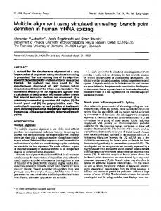
International Journal of Computer Applications (0975 – 8887) Volume 6– No.2, September 2010 (PC). The differential pressure transmitter is been calibrated to read the level of 0-43 cm in the conical tank in terms of 4-20 mA and this current output from the DPT is passed through 100 ohms resistance and thus converted into 0.4 – 2 V. This voltage at the input of ADC of ADAM module is interfaced with computer through the RS-232 port of the PC. The output current signal of the DAC is given to a current to pressure (I/P) converter which is connected to the pneumatic control valve. The inflow rate is thus adjusted by changing the stem position of the control valve from fully open to fully close. The control signal from the PC is transmitted to the I/P converter in the form of current signal (420) mA, which converts it to corresponding 3-15 psi of compressed air; further given as input to the pneumatic control valve. The pneumatic control valve is actuated by this signal to produces the required flow rate of water in the conical tank to maintain its level. The ADAM’s module has 8 analog input and 4 analog output channels with the voltage range of ±10 volt. The sampling rate of the module is 18 samples per sec and baud rate is 9600 bytes per sec with 16-bit resolution. The programs written in m-file of MATLAB software is then linked via ADAM’s module with the sampling time of 60 milliseconds. The photograph of the experimental setup is given in the figure.1,and its technical details is given in table.1.
2.2 Step Testing Method Step response based methods are most commonly used for system identification, especially in process industries. To get an effective and accurate mathematical model, this method requires the conical tank level response, assumption of a suitable model and estimates of model parameters. The selection of the model could be based on the shape of the open-loop step response. The open loop step response is obtained by varying the manual mode output from the controller with the optimal value of flow through the control valve so that the response can be validated for the entire range. A large number of graphical methods are available in literature and they have been used effectively in real time applications to obtain the model. In this project we are implementing the SunderasanKumaraswamymethod[15] to validate the model from the obtained response. As per the structure of the curves, we predict the model to be of the form similar to first order plus time delay (FOPTD), and hence the model is given by Ke-
G(s) =
ds
s+1 where K = process gain first order time constant d
= delay time
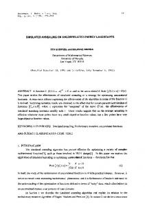
From the response of the real time system we obtain the mentioned constants and thereby we get the FOPTD models for the real time spherical tank process as G(s) = 6.86e-4.73s 219.76s+1 For the obtained FOPTD model the step change of similar magnitude is given and simulated using MATLAB. The response of the model was compared and it was found that the simulation for the proposed model had a response that was close to the real time response and is as shown in figure.2. real time
Fig.1. Photograph of Experimental Setup Table.1. Technical details of the various transducers in the experimental setup
model
60 50 40
PART NAME
DETAILS
Spherical tank Stainless Steel, Diameter - 48 cm Differential pressure transmitter
Capacitance type, Range 2.5 - 250mbar, Output4 - 20mA
Pump
Centrifugal 0.5 HP
Control valve
Size ¼“ Pneumatic actuated, Type: Air to close, Input 3 - 15 psi
Rotameter
Range 0 - 18 lpm
Air regulator
Size 1/4" BSP,Range 0 - 2.2 bar
I/P converter
Input 4-20 mA, Output 0.2 - 1 bar
30 20 10 0 -10
Pressure gauge Range 0 - 30 psi
0
200
400
600
800
1000
1200
Fig .2. Comparison of real time and simulated responses for proposed model
2.3 CONVENTIONAL DESIGN TECHNIQUES The basic PI controller parameters are given as, proportional gain, Kp and integral gain Ki. Over the last fifty years, numerous methods have been developed for setting the parameters of a PID controller [10]. In this paper it is considered to proceed the tuning with traditional tuning methodology, using Internal Model Control 21
International Journal of Computer Applications (0975 – 8887) Volume 6– No.2, September 2010 (IMC) tuning technique proposed by Skogestad [4] for PI tuning The IMC technique is one of the recent traditional tuning techniques that yields better values among the techniques available for conventional methods. For a FOPTD model of the mentioned form in equation (1) the IMC tuning values based on Skogestad proposal is given as Kp= 1 ( c + d ) where c = d as per Skogestad, K and integral time constant Ti is given as ,Ti = Applying the technique we get the IMC tuning parameters as Kp= 3.2904 ,Ki = 0.015 for the proposed model.
the Metropolis algorithm, there is some finite probability of selecting the point x(t+1) even though it is a worse than the point x (t) .The principle is represented in figure.3.The new stateK1is accepted, but the new state K2is only accepted with a certain probability.
3. SA based controller 3.1 Simulated Annealing: SA is a numerical optimization technique based on the principles of thermodynamics. The Simulated Annealing method resembles the cooling process of molten metals through annealing. At high temperature, the atoms in the molten metal can move freely with respect to each another. But, as the temperature is reduced, the movement of the atoms gets reduced. The atoms start to get ordered and finally form crystals having the minimum possible energy. However, the formation of the crystal depends on the cooling rate. If the temperature is reduced at a very fast rate, the crystalline state may not be achieved at all; instead the system may end up in a polycrystalline state, which may have a higher energy state than the crystalline state. Therefore in order to achieve the absolute minimum state, the temperature needs to be reduced at a slow rate. The process of slow cooling is known as annealing in metallurgical parlance. SA simulates this process of slow cooling of molten metal to achieve the minimum function value in a minimization problem. The cooling phenomenon is simulated by controlling a temperature-like parameter introduced with the concept of the Boltzmann probability distribution. According to the Boltzmann probability distribution, a system in thermal equilibrium at a temperature T has its energy distributed probabilistically according to
Fig.3. Selection of new states in SA The probability of accepting a worse state is high at the beginning and decreases at the temperature decreases. For each temperature, the system must reach an equilibrium i.e., a number of new states must be tried before the temperature is reduced typically by 10 %. It can be shown that the algorithm will find, under certain condition, the global minimum and not get stuck in local minima. Figure 4.iIllustrates the flowchart of SA algorithm.
P (E) = exp (- ∆E / kT), where k is the Boltzmann constant. This expression suggests that a system at a high temperature has almost uniform probability of being at any energy state, but at a low temperature it has a small probability of being at a high energy state. Therefore, by controlling the temperature T and assuming that the search process follows the Boltzmann probability distribution, the convergence of an algorithm can be controlled using the Metropolis algorithm. At any instant the current point is x (t) and the function value at that point is E (t) = f (x(t)). Using the Metropolis algorithm, the probability of the next point being at x (t+1) depends on the difference in the function values at these two points or on E = E(t+1)–E(t) and is calculated using the Boltzmann probability distribution: P ( E (t+1) ) = min [1, exp ( - E/kT)]. If E 0, this probability is one and the point x (t+1) is always accepted. In the function minimization context, this makes sense because if the function value at x (t+1) is better than that at x(t), the point x (t+1) must be accepted. When E > 0, which implies that the function value at x(t+1) is worse than that at x(t). According to
Fig. 4. Flowchart for SA algorithm 22
International Journal of Computer Applications (0975 – 8887) Volume 6– No.2, September 2010
4. IMPLEMENTATION OF SA ALGORITHM
5
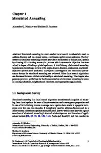
Distribution of Kp
The optimal values of the conventional PI controller parameters Kp and Ki,is found using SA. All possible sets of controller parameter values are particles whose values are adjusted so as to minimize the objective function, which in this case is the error criterion, which is discussed in detail.For the PI controller design, it is ensured the controller settings estimated results in a stable closed loop system.
6
3 2 1 0
4.1 Selection of SA parameters
0
20
40
0.045
0.03
0.015
0 0
20
40
4.2 Performance Index for the SA Algorithm The objective function considered is based on the error criterion. The performance of a controller is best evaluated in terms of error criterion. A number of such criteria are available and in this paper, controller’s performance is evaluated in terms of Integral of Absolute Errors (IAE ) criterion, given by
60
80
100
initial iteration
Fig 6. Distribution of Ki in first iteration For each iteration the best among the 100 particles considered as potential solution are chosen. Therefore the best values for 100 iterations is sketched with respect to iterations for Kp and Ki, and are as shown in figure 7 & 8. 6 5 4
Kp
Multiplication Factor – (Ti - Td)/ Ti = 0.995
100
0.06
Initial Temperature- 1500 Termination temperature- 0.001
80
Fig 5. Distribution of Kp in first iteration
Population size – 100 Decrement Temperature- 10
60
initial iteration
Distribution of Ki
To start up with SA, certain parameters need to be defined. It includes initial temperature (Ti), decrement temperature (Td), population size, terminating temperature (Tt), multiplication factor etc. Selection of these parameters decides to a great extent the ability of global minimization. The initial temperature and decrement factor, through the multiplication factor decides the number of iterations that affect the ability of escaping from local optimization and refining global optimization. In this work the parameters are so selected to have 100 iterations. The population size balances the requirement of global optimization and computational time. The range of the tuning parameters is considered in the range of 0-10.Initializing the values of the parameters for this paper is as follows:
4
3 2 1 0
The IAE weights the error with time and hence emphasizes the error values over arrange of 0 to T, where T is the expected settling time
0
20
60
80
100
Fig.7. Best solutions of Kp for 100 iterations.
4.3 Termination Criteria 0.06 0.05 0.04 0.03
Ki
Termination of optimization algorithm can take place either when the maximum number of iterations gets over or with the attainment of satisfactory fitness value. Fitness value is nothing but reciprocal of the magnitude of the objective function, since we consider for a minimization of objective function. In this paper the termination criteria is considered to be the attainment of satisfactory fitness value which occurs with the maximum number of iterations as 100.Application of the SA algorithm with IAE error criterion for 100 iterations gives us the variation of the PI parameters. For each iteration the best of the 100 solutions chosen is considered . The variation of the values for the first iteration for Kp and Ki are given below for the model as shown in Figure 5 & 6. It is clearly seen that the values are distributed.
40
number of iterations
0.02 0.01 0 -0.01
0
20
40
60
80
100
number of iterations
Fig.8. Best solutions of Ki for 100 iterations. The PI controller were formed based upon the respective 23
International Journal of Computer Applications (0975 – 8887) Volume 6– No.2, September 2010 parameters for 100 iterations, and the gbest (global best) solution was selected for the set of parameters, which had the minimum error. A sketch of the error based on IAE criterion for 100 iterations is as given in figure.9.
Table.2.Comparison of time domain specifications for the real time response. IMC controller SA controller
700 600 500
IAE
The real time results clearly infer that the SA tuned controller performs better than the IMC tuned controller for a set of 15 cm.The time domain specifications for the real time responses is given in table.6.
400
Rise time (seconds)
200
149
Peak time (seconds)
256
183
Overshoot (%)
9.13
2.87
Settling time (seconds)
289
208
300 200 100 0 0
20
40
60
80
100
number of iterations
Fig.9. IAE values for 100 iterations It was seen that the error value tends to decrease for a larger number of iterations. As such the algorithm was restricted to 100 iterations for beyond which there was only a negligible improvement. Based on SA algorithm for the application of the PI tuning we get the PI tuning parameters for model 1 as Kp=4.416,Ki = 0.0158
5. RESULTS AND COMPARISON The tuned values through the traditional as well as the proposed techniques are analysed for their responses to a unit step input, with the help of simulation and then the real time application for the spherical tank is presented. A tabulation of the time domain specifications comparison and the performance index comparison for the obtained models with the designed controllers is presented. Further robustness investigation is done by varying the model parameters by twenty percent.
5.1 Real time response of the experimental setup for set point conditions
SA
16 12
level(cm)
The PI controllers tuned by the PSO based method should not be compared only with their time domain responses but also with its performance index from the four major error criterion techniques of Integral Time of Absolute Error(ITAE) ,Integral of Absolute Error(IAE) ,Integral Square of Error(ISE )and Mean Square Error (MSE).Robustness of the controller is defined as its ability to tolerate a certain amount of change in the process parameters without causing the feedback system to go unstable. In order to investigate the robustness of the proposed method in the face of model uncertainities, the model parameters were altered. Here the value of gain constant K, time constant, , and delay time d is deviated by as much as ±20% of its nominal values. In the proposed models for the experimental setup the value of K is incremented by 20 %, the value of , is incremented by 20 % and that of d is reduced by 20%.Thus the model with the proposed uncertainities is G(s) = 8.228e-3.89s
The most important aspect of the paper is presented in this section.The real time response of the system were observed by giving a set point of 15 cm, and the corresponding variation of level from a reference value of zero was recorded .The outflow valve from the tank was kept partially open and the position was retained for the various trials of controller settings. The response of the spherical tank for set point of 15 cm with various controller settings are presented as shown in figure.10. IMC
5.2 Robustness Investigation:
263.71s+1 For the proposed model the comparison of performance index were done and are listed as per the given table Table.3 Comparison of performance index for 20% changes in model parameters IMC controller SA controller ITAE
562.69
261.11
IAE
97.36
70.81
ISE
73.41
60.15
MSE
0.1465
0.1201
8
6. CONCLUSION
4 0 0
50
100
150
200
250
time(seconds)
Fig.10.Real time response for a set point of 15 cm
300
The various results presented prove the betterness of the SA tuned PI settings than the IMC tuned ones. The simulation responses for the models validated reflect the effectiveness of the SA based controller in terms of time domain specifications. The performance index under the various error criterions for the proposed controller is always less than the IMC tuned controller. 24
International Journal of Computer Applications (0975 – 8887) Volume 6– No.2, September 2010 Above all the real time responses confirms the validity of the proposed SA based tuning for the spherical tank. SA presents multiple advantages to a designer by operating with a reduced number of design methods to establish the type of the controller, giving a possibility of configuring the dynamic behavior of the control system with ease, starting the design with a reduced amount of information about the controller (type and allowable range of the parameters), but keeping sight of the behavior of the control system. These features are illustrated in this paper by considering the problem of designing a control system for a plant of first-order system with time delay and deriving the possible results. The future scope of the work is aimed at providing an on-line self tuning PI controller with the proposed algorithm so as solve complex issues for real time problems.
7.
8.
9. 10. 11.
7. REFERENCES 1.
2. 3.
4. 5.
6.
Hsien-Yu Tseng and Chang-Ching Lin, "A simulated annealing approach for curve fitting in automated manufacturing systems", Journal of Manufacturing technology management, Vol 18, No.2 pp. 202-216, 2007 PierpaoloCaricato and Antonio Grieco, “Using simulated annealing to design a material handling system”, IEEE intelligent systems, 2005. Li-Sun Shu, Shinn-Ying Ho and Shinn-Jang Ho, “A novel orthogonal simulated annealing algorithm for optimization of electromagnetic problems.”, IEEE transactions on Magnetics, Vol.40, No. 4, July 2004. SigurdSkogestad, “Simple analytic rules for model reduction and PID controller tuning”, Journal of Process Control 13 (2003) 291–309,2003. L.R.Varela, R.A.Ribeiro and F.M.Pires, “Simulated annealing and fuzzy optimization”, Proceedings of the 10th Mediterranean conference on control and automation- MED2002,Portugal, July 9-12, 2002. JavedAlam Jan and BohumilSulc, “Evolutionary computing methods for optimizing virtual reality process models”, International Carpathian control conference ICCC’2002, Malenovice Czech republic, May 27-30, 2002.
12.
13.
14.
15.
16.
S.Chen, R.H. Istepanian and J.Wu, “ Optimizing stability bounds of finite-precision PID controllers using adaptive simulated annealing”, Proceedings of the American control conference ,San Diego, California ,June 1999. S. Chen and B.L.Luk, "Adaptive simulated annealing for optimization in signal processing applications", Journal of Engineering and electronics, Vol. 79,pp. 117128, 1999. Yan Tian, Li Erxue and Yang Shiyou, “Improved simulated annealing algorithm and its application in fault-location of power transmission lines”, IEEE 1998. Luyben, W.L and M.L Luyben, “Essentials of process control”, McGraw-Hill, New York (1997). Simon Fabri and VisakanKadirkamanathan, “Dynamic structure neural networks for stable adaptive control of nonlinear systems”, IEEE transactions on neural networks, Vol 7, No. 5, September1996. Sanjay I. Mistry, Shao-liang Chang and Satish S. Nair, “Indirect control of a class of nonlinear dynamic systems”, IEEE transactions on neural networks Vol 7, No. 4, July 1996. Mehrdad Salami and Greg Cain, “An adaptive PID controller based on Genetic algorithm processor”, Genetic algorithms in engineering systems:Innovations and applications 12-14 September 1995, Conference publication No. 414, IEE 1995. Su Whan Sung, In-Beum Lee and Jitae Lee,“ Modified Proportional-Integral Derivative (PID) Controller and a New Tuning Method for the PID Controller”,Ind. Eng.Chem. Res.,34, 4127-4132, 1995. Sundaresan,K.R.,Krishnaswamy,R.R.,“Estimation of time delay, time constant parameters in Time, Frequency and Laplace Domains”, Journal of Chemical Engineering.,56,257,1978. J. G. Ziegler and N. B. Nichols, “Optimum settings for automatic controllers,” Trans. Amer. Soc. Mech. Eng., vol. 64, pp. 759–768, 1942
25