Downloaded By: [Brown University] At: 04:47 3 April 2007
Cybernetics and Systems: An International Journal, 38: 187–202 Copyright Q 2007 Taylor & Francis Group, LLC ISSN: 0196-9722 print=1087-6553 online DOI: 10.1080/01969720601139058
DESIGN OF DECISION TREE VIA KERNELIZED HIERARCHICAL CLUSTERING FOR MULTICLASS SUPPORT VECTOR MACHINES
ZHAO LU Department of Naval Architecture and Marine Engineering, University of Michigan, Ann Arbor, MI, USA FENG LIN HAO YING Department of Electrical and Computer Engineering, Wayne State University, Detroit, MI, USA
As a very effective method for universal purpose pattern recognition, support vector machine (SVM) was proposed for dichotomic classification problem, which exhibits a remarkable resistance to overfitting, a feature explained by the fact that it directly implements the principle of structural risk minimization. However, in real world, most of classification problems consist of multiple categories. In an attempt to extend the binary SVM classifier for multiclass classification, decision-tree-based multiclass SVM was proposed recently, in which the structure of decision tree plays an important role in minimizing the classification error. The present study aims at developing a systematic way for the design of decision tree for multiclass SVM. Kernel-induced distance function between datasets was discussed and then kernelized hierarchical clustering was developed and used in determining the structure of decision tree. Further, simulation results on satellite image interpretation show the superiority of the proposed classification strategy over the conventional multiclass SVM algorithms. Address correspondence to Hao Ying, Department of Electrical and Computer Engineering, Wayne State University, Detroit, MI 48202. E-mail:
[email protected]
188
Z. LU ET AL.
Downloaded By: [Brown University] At: 04:47 3 April 2007
INTRODUCTION Most of the learning algorithms proposed in the past 20 years had been based, to a large extent on heuristics or on loose analogies with natural learning systems, such as the concept of evolution, or models of nervous systems. As a new generation of learning algorithms, kernel methods utilize techniques from optimization, statistics, and functional analysis to achieve maximal generality, flexibility, and performance. These algorithms have more in common with statistical methods than with classical artificial intelligence, and are quite different from earlier techniques used in machine learning in many respects. For example, they are explicitly based on a theoretical model of learning rather than on loose analogies with natural learning systems or other heuristics. They come with theoretical guarantees about their performance and have a modular design that makes it possible to separately implement and analyze their components. They are not plagued with the problem of local minima because their training amounts to convex optimization. As a result, there is a trend in recent machine learning community to construct a nonlinear version of linear algorithm using the ‘‘kernel method’’ (Mu¨ller et al. 2001; Scho¨lkopf and Smola 2002), such as SVM (Vapnik 1998; Cristianini and Shawe-Taylor 2000), kernel principal component analysis (KPCA) (Scho¨lkopf et al. 1998), kernel fisher discriminant (KFD) (Roth and Steinhage 1999; Baudat and Anouar 2000) and the recent kernel clustering algorithm (Girolami 2002; Zhang and Chen 2004). The kernel allows high-dimensional inner product computations to be performed with very little overhead and brings all the benefits of linear estimation. The beauty of the result is its simplicity and ease of application that makes it attractive to practitioners. The SVM, pioneered by Vapnik, is known as an excellent tool for classification and regression problems with a good generalization performance. Contrary to the neural networks, which followed a more heuristic path, SVM started with fundamental theoretical framework and then evolved to their implementation and experimental work. An SVM is intrinsically a binary classifier, which constructs the discriminant function from a set of labeled patterns called training examples. Let ðXi ; yi Þ 2 Rn # f$1g; i ¼ 1; . . . ; l be such a set of training examples. The purpose is to select a function f : Rn ! f$1g from a given class of functions ffa : a 2 Kg such that f will correctly classify test examples ðX ; yÞ. If the decision surface f was estimated by only using the empirical
Downloaded By: [Brown University] At: 04:47 3 April 2007
MULTICLASS SUPPORT VECTOR MACHINES
189
risk minimization, even a function that performs well with training data may not generalize well to unseen data. Hence, just minimizing the training error does not imply a small test error averaged over test data. Adding an additional requirement that the optimal hyperplane should have good generalization properties can help choose the best hyperplane. The structural risk minimization principle imposes structure on the optimization process by ordering the hyperplanes based on the margin. The optimal hyperplane is the one that maximizes the margin while minimizing the empirical risk. This indirectly ensures better generalization. On the other hand, in real world, most of classification problems consist of multiple categories, such as handwritten character recognition, face detection, and so on. Hence, how to extend the binary SVM classifier for multiclass classification is an important issue. To this end, a variety of approaches have been proposed (Weston and Watkins 1999; Hsu and Lin 2002). These approaches fall into two categories. The first approach denoted as all-in-one is to directly consider all data in one optimization formulation, which is a straightforward generalization of the support vector concept to more than two classes. The second one denoted as divideand-combine is to decompose the multiclass problem into several subproblems that can be solved by binary SVMs. The output of these SVMs are incorporated together to produce the final output. The main problem associated with the all-in-one approach is that it may result in solving a quadratic programming problem with a large number of variables, which requires prohibitively expensive computing resources for many real-world problems. Within the ‘‘divide-and-combine’’ approach, two widely used methods are to divide the problem. One of them is called one-against-all method. Suppose we have a k-class pattern employed recognition problem. Then, k independent SVMs are constructed and each of them is trained to separate one class of samples from all others. When testing the system after all the SVMs are trained, a sample is chosen as input to all the SVMs. If this sample belongs to class p, then ideally only the SVM trained to separate class p from the others should have a positive response. But in many practical applications, there may be multiple positive responses and in those cases we choose the SVM with the largest output. The major drawback of this heuristic is that, it does not yield optimal decision boundaries which could be obtained by simultaneous optimization of all borders. Moreover, by this formulation unclassifiable regions exist.
Downloaded By: [Brown University] At: 04:47 3 April 2007
190
Z. LU ET AL.
Another method is called pairwise method, in which a k-class problem is converted into kðk & 1Þ=2 two-class problems which cover all pairs of classes. SVMs are constructed and each of them is trained to separate one class from another class, and then the classification decision for a test sample is based on the aggregate of output magnitudes. In most cases, the pairwise method outperforms the one-versusothers. However, by this method also, unclassifiable regions exist. For multiclass classification, top-down induction of decision trees is a simple and powerful method of inferring classification rules from a set of labeled examples. Recently, binary-tree-based multiclass SVM was proposed (Cheong et al. 2004; Abe 2005), which can be viewed as a new member in the family of ‘‘divide-and-combine’’ methods. This approach takes advantage of both the efficient computation of the hierarchical tree architecture and the high classification accuracy of SVMs. The binary tree based multiclass SVM has several aspects superior to the conventional methods. For k-class problem, only k & 1 hyperplanes need to be calculated, i.e., the number of dichotomic SVMs to be trained is less than that in one-against-all and pairwise methods. Moreover, as learning proceeds, the number of data involved in dichotomic SVM training decreases rapidly, hence shorter training time can be expected. In the testing phase, all decision functions need to be computed in the conventional methods. In contrast, only log2 k decision functions need to be calculated in the binary tree based multiclass SVM. Particularly, the problem of unclassified region was completely surmounted in this approach. At each node of the binary tree, the decision is made to assign the input pattern into one of two groups, which consist of multiple classes. There exist many ways to divide the multiple classes into two groups. Hence, the structure of the binary tree, which determines how to partition the multiple classes at each nonleaf node, is critical to the overall classification performance of the algorithm. In this article, it is from the perspective of the dissimilarity of classes that the distance functions between datasets are discussed. Particularly, given the fact that SVMs implement classification implicitly in the feature space, the kernelized hierarchical clustering algorithm was developed and used in constructing the binary tree for multiclass SVM. This paper is organized as follows. In the next section, a brief review about binary SVM classification is given. Following that, the kernel-induced distances between datasets are investigated; and then
Downloaded By: [Brown University] At: 04:47 3 April 2007
MULTICLASS SUPPORT VECTOR MACHINES
191
the algorithm for design of decision tree via kernelized hierarchical clustering is developed. Finally, the simulation study on satellite image data is demonstrated with the concluding remarks. SUPPORT VECTOR MACHINES FOR BINARY CLASSIFICATION Basically, the SVM is a linear machine working in the highly dimensional feature space formed by the nonlinear mapping of the n-dimensional input vector X into a m-dimensional feature space (m > n) through the use of a mapping of UðX Þ. The equation of the hyperplane separating two different classes is given by the relation f ðX Þ ¼ W T UðX Þ þ b ¼ 0; where UðX Þ ¼ ½u1 ðX Þ; u2 ðX Þ; . . . ; um ðX Þ)T and W ¼ ½w1 ; w2 ; . . . ; wm )T . W and b are the weights of the support vector network. The SVM approach consists in finding the optimal hyperplane that maximizes the distance between the closest training sample and the separating hyperplane. It is possible to express this distance as equal to 1=kW k with a simple rescaling of the hyperplane parameters W and b such that min
i¼1;2;...;l
yi ðW * UðXi Þ þ bÞ + 1
The geometrical margin between the two classes is given by the quantity 2=kW k. The concept of margin is central in the SVM approach, since it is a measure of its generalization capability. The larger the margin, the higher is the expected generalization capability. Accordingly, it turns out that the optimal hyperplane can be determined as the solution of the following convex quadratic programming problem: (
minimize : 12 kW k2
subject to : yi ðW * UðXi Þ þ bÞ + 1; i ¼ 1; 2; . . . ; l
Further, to accommodate the dataset, which are not linearly separable in the feature space, the slack variables ni were introduced into the primal optimization formulation, which result in the following soft margin
Downloaded By: [Brown University] At: 04:47 3 April 2007
192
Z. LU ET AL.
SVM classifier: 8 l P > 2 > 1 > ni < minimize : 2 jjW jj þ C i¼1
> > subject to : yi ðW * UðXi Þ þ bÞ + 1 & ni ; > : ni + 0; i ¼ 1; 2; . . . ; l
ð1Þ
where C is a parameter that determines the tradeoff between the maximum margin and the minimum classification error. Here, the separability constraints were relaxed and each exceeding of the constraints will be punished by a misclassification penalty (i.e., an increase in the primal objective function). Using the Lagrangian, the classical linearly constrained optimization problem (1) can be reduced to the following dual problem by introducing the Lagrange multiplier ai : 8 l P l l P 1P > > > < minimize: 2 i¼1 j¼1 ai aj yi yj hUðXi Þ; UðXj Þi & i¼1 ai l > P > > : subject to : ai yi ¼ 0 and 0 , ai , C; i¼1
i ¼ 1; 2; . . . ; l
which is a quadratic programming problem. The Lagrange multiplier ai ’s ði ¼ 1; 2; . . . ; lÞ in the expression above can be estimated using quadratic programming methods, and the kernel function was defined in the form of inner product KðXi ; Xj Þ ¼ hUðXi Þ; UðXj Þi that allows a dot product to be computed in a higher dimensional feature space without explicitly mapping the data into these spaces. The feature space has the structure of a reproducing kernel Hilbert space and hence minimization of jjW jj2 can be understood in the context of regularization operators. The kernel-based decision surface can be expressed by an equation depending both on the Lagrange multipliers and on the training samples, i.e., ! X f ðX Þ ¼ sign ai yi KðXi ; X Þ þ b i2S
where S is the subset of training samples corresponding to the nonzero Lagrange multipliers ai ’s. It is worth noting that the Lagrange multipliers effectively weight each training sample according to its importance in determining the
Downloaded By: [Brown University] At: 04:47 3 April 2007
MULTICLASS SUPPORT VECTOR MACHINES
193
decision surface. The training samples associated to nonzero weights are called support vectors. These lie at a distance exactly equal to 1=kW k from the optimal separating hyperplane. The threshold b can be computed by means of the Karush-Kuhn-Tucker (KKT) conditions, and averaging over the support vectors Xj with aj < C (the training examples Xj with nonzero slack variables correspond to aj ¼ C) yields a numerically stable solution: ! X 1 X b¼ yj & ai yi KðXi ; Xj Þ jSj j2S i2S where j*j denotes the size of set. KERNEL-INDUCED DISTANCE BETWEEN DATASETS In order to pave the way for the kernelized hierarchical clustering algorithm, the distance measure characterizing the dissimilarity between classes needs to be defined beforehand. Firstly, let us recall the notion of metric. A distance measure d is called a metric when the following conditions are fulfilled: . . . .
reflectivity, i.e., dðX ; X Þ ¼ 0 positivity, i.e., dðX ; Y Þ > 0 if X is distinct from Y symmetry, i.e., dðX ; Y Þ ¼ dðY ; X Þ triangle inequality, i.e., dðX ; Y Þ , dðX ; ZÞ þ dðZ; Y Þ for every Z
Reflectivity and positivity are crucial to define a proper dissimilarity measure (Pekalsak et al. 2001). The function d is a distance function if it satisfies reflectivity, positivity and symmetry. Given that the SVMs calculate the separate hyperplane implicitly in the feature space, it is necessary and natural to define the measure of dissimilarity in the feature space. For the points X and Y in the input space, the Euclidean distance between them in the feature space was defined as: dðX ; Y Þ ¼ kUðX Þ & UðY Þk
ð2Þ
where k*k is the Euclidean norm, and U is the implicit nonlinear map from the data space to feature space. As seen above, by using the kernel K, all computations can be carried out implicitly in the feature space that U maps into, which can have a very high (maybe infinite) dimensionality.
194
Z. LU ET AL.
Downloaded By: [Brown University] At: 04:47 3 April 2007
Three commonly used kernel functions in literature are: . Gaussian radial basis function (GRBF) kernel: & kX & Y k2 KðX ; Y Þ ¼ exp r2
!
. Polynomial kernel: KðX ; Y Þ ¼ ð1 þ hX ; Y iÞq . Sigmoid kernel: KðX ; Y Þ ¼ tanh ðahX ; Y i þ bÞ where r, q, a, b are the adjustable parameters of the above kernel functions. For the sigmoid function, only a set of parameters satisfying the Mercer theorem can be used to define a kernel function. The kernel function provides an elegant way of working in the feature space avoiding all the troubles and difficulties inherent in high dimensions, and this method is applicable whenever an algorithm can be cast in terms of dot products. In light of this, we expressed the distance (2) in the entries of kernel (Pekalsak 2001; Scho¨lkopf 2001), kUðX Þ & UðY Þk2 ¼ ðUðX Þ & UðY ÞÞT ðUðX Þ & UðY ÞÞ
¼ UðX ÞT UðX Þ & UðY ÞT UðX Þ & UðX ÞT UðY Þ þ UðY ÞT UðY Þ
¼ KðX ; X Þ þ KðY ; Y Þ & 2KðX ; Y Þ
ð3Þ
Consequently, the distance (2) can be computed without explicitly using or even knowing the nonlinear mapping U, and it can be defined as the kernel-induced distance in the input space. Below we confine ourselves to the Gaussian RBF kernel, so KðX ; X Þ ¼ 1. Thus, we arrive at kUðX Þ & UðY Þk2 ¼ 2 & 2KðX ; Y Þ
ð4Þ
Further, for the sake of measuring the dissimilarity between classes in the feature space, a kernel-induced distance between datasets in the input space needs to be defined. The best known metric between subsets of a metric space is the Hausdorff metric, which is defined as the maximum distance between any point in one shape and the point that
Downloaded By: [Brown University] At: 04:47 3 April 2007
MULTICLASS SUPPORT VECTOR MACHINES
195
is closest"to !it in the other. #That is, for point sets A ¼ fai ji ¼ 1; 2; . . . ; pg and B ¼ bj ! j ¼ 1; 2; . . . ; q , it is % & $ $ $ $ dh ðA; BÞ ¼ max max min$ai & bj $; max min$ai & bj $ ai 2A bj 2B
bj 2B ai 2A
This metric is trivially computable in polynomial time, and it has some quite appealing properties. However, it is evident that Hausdorff metric is not very well suited for some classification applications because the Hausdorff distance does not take into account the overall structure of the point sets. In an attempt to surmount this problem, we employed the sum of minimum distances function dmd as follows (Eiter and Mannila 1997) 0 1 $ $ X $ $ 1 @X dmd ðA; BÞ ¼ min$ai & bj $ þ min$ai & bj $A ai 2A 2 a 2A bj 2B b 2B i
j
For measuring the degree of dissimilarity between two datasets in the feature space, we consider the kernel-induced sum of minimum distance function d~md 0 1 X X $ $ $ $ 1 d~md ðA; BÞ ¼ @ min$Uðai Þ & Uðbj Þ$ þ min$Uðai Þ & Uðbj Þ$A ai 2A 2 a 2A bj 2B b 2B i
j
ð5Þ
Obviously, by the formulation of Eq. (3), the distance Eq. (5) can also be expressed only in the entries of kernel. If Gaussian RBF kernel was chosen as the kernel function, by using Eq. (4) d~md can be recast into 0 1 qffiffiffiffiffiffiffiffiffiffiffiffiffiffiffiffiffiffiffiffiffiffiffiffiffiffiffiffi X qffiffiffiffiffiffiffiffiffiffiffiffiffiffiffiffiffiffiffiffiffiffiffiffiffiffiffiffi X 1 d~md ðA; BÞ ¼ @ min 2 & 2Kðai ; bj Þ þ min 2 & 2Kðai ; bj ÞA ai 2A 2 a 2A bj 2B b 2B i
j
which implies that it can be calculated without knowing the nonlinear mapping U DESIGN OF DECISION TREE VIA KERNELIZED HIERARCHICAL CLUSTERING
For the purpose of utilizing the training algorithm of dichotomic SVM, the binary decision tree was used in solving the k-class pattern recognition problem.
Downloaded By: [Brown University] At: 04:47 3 April 2007
196
Z. LU ET AL.
Figure 1. Binary tree-based multiclass support vector machines.
As shown in Figure 1, each node of the binary tree implements a binary discrimination with an SVM that splits the examples into two partitions. The region of each class hinges on the structure of a decision tree; hence, it is necessary to determine the structure of the binary tree before the training of each SVM classifier so that the classification error is minimized. Given the hierarchical architecture of binary decision tree, if the classification performance degrades at the upper node of the binary tree, the overall classification performance becomes worse. Therefore, the structure of binary tree plays an important role in minimizing the classification error, and classes that are more separable should be partitioned at the upper node of the decision tree. Thus, an unsupervised learning problem arises in constructing the binary tree. As a principal approach to unsupervised learning, hierarchical clustering (Theodoridis and Koutroumbas 1998; Webb 2002) was adopted in determining the architecture of decision tree. In hierarchical clustering the data are not partitioned into a particular cluster in a single step. Instead, a series of partitions take place, which may run from a single cluster containing all objects to k clusters, each containing a single object. Hierarchical clustering is subdivided into agglomerative methods, which proceed by series of fusions of the n objects into groups, and divisive methods, which separate n objects successively into finer groupings.
Downloaded By: [Brown University] At: 04:47 3 April 2007
MULTICLASS SUPPORT VECTOR MACHINES
197
In this article, taking into account the fact that the discrimination hyperplane in SVM was computed implicitly in the feature space by kernel trick, the kernelized hierarchical divisive clustering was developed and exploited in determining the structure of the binary tree. By means of the kernel-induced distance function between datasets, which measures the dissimilarity between classes, the algorithm was described as follows: First, choose the kernel functions to be used for dichotomic SVM and for computing the kernel-induced distance in every node. This provides a chance to use different kernels in different nodes, which enhance the flexibility of the multiclass classifier. Then, starting from the root node and successively for every nonleaf node by traversing the tree, the kernelized hierarchical divisive clustering was used in partitioning the datasets for a specified nonleaf node: compute the kernel-induced sum of minimum distance function d~md between all pairs of the datasets in the corresponding nonleaf node; partition the datasets pair between which the distance is maximal into the left node and right node as the prototype dataset of the child node, respectively. Subsequently, assign the remaining datasets into the corresponding child node whose prototype dataset is the closest to it in the sense of kernel-induced distance function. Repeat this procedure until every leaf-node was reached. Thus, the overall structure of binary decision tree was determined, which is easily interpretable and can provide insight into the data structure. Based on the structure of the binary decision tree, on each nonleaf node, the samples from the datasets in its left child node and its right child node can be relabeled as þ1 and &1, respectively. Then, the multiclass SVM classifier can be obtained by training the binary SVM for every nonleaf node, which implements a decision rule that separate the samples belonging to the datasets in its left node from those belonging to the datasets in its right node. For an k-class problem, the number of hyperplanes to be calculated is k & 1. It is less than that of the conventional methods. As learning proceeds, the number of data involved in training becomes smaller, so the shorter training time can be expected. For classification of the unlabeled data by making use of the obtained multiclass SVM, the procedure starts from the root node of the decision tree; the value of the decision function for input data Xi can be calculated and then according to the sign of the value we determine which node to go to. We iterate this procedure until we reach a leaf node and classify the input into the class associated with the node.
Downloaded By: [Brown University] At: 04:47 3 April 2007
198
Z. LU ET AL.
Contrary to the conventional methods, in which the values for all the decision functions need to be calculated at the stage of classification, the values of all the decision functions are not necessarily calculated in the proposed method, though it depends on the structure of the decision tree. LANDSAT SATELLITE IMAGE DATA CLASSIFICATION In this section, the proposed method was applied on the recognition of satellite image data (King et al. 1995). The experimental result was compared with those acquired from other pattern classification methods and conventional multiclass SVM algorithms by making use of the statistical pattern recognition toolbox (Franc and Hlavac 2004). A recommended test dataset was provided, thus making fair comparison with other algorithms feasible. The satellite image database was generated by taking a small section from the original Landsat multi-spectral scanner (MSS) image data from a part of western Australia. The interpretation of a scene by integrating spatial data of diverse types and resolutions including multispectral and radar data, maps indicating topography, land use, etc. is expected to assume significant importance with the onset of an era characterized by integrative approaches to remote sensing. One frame of Landsat MSS imagery consists of four digital images of the same scene in different spectral bands. Two of these are in the visible region (corresponding approximately to green and red regions of the visible spectrum) and two are in the (near) infra-red. Each pixel is a 8-bit binary word, with 0 corresponding to black and 255 to white. The spatial resolution of a pixel is about 80 m # 80 m. Each image contains 2340 # 3380 such pixels. The database is a (tiny) subarea of a scene, consisting of 82 # 100 pixels. Each line of data corresponds to a 3 # 3 square neighborhood of pixels completely contained within the 82 # 100 subarea. Each line contains the pixel values in the four spectral bands (converted to ASCII) of each of the nine pixels in the 3 # 3 neighborhood and a number indicating the classification label of the central pixel. Hence, each sample was featured by 36 attributes, which are numerical in the range 0–255. Namely, the input space is of 36 dimensions. Totally, we have 4435 samples in the training dataset, and 2000 samples in the testing dataset. There are six classes of different soil conditions to be classified as shown in Table 1.
MULTICLASS SUPPORT VECTOR MACHINES
199
Downloaded By: [Brown University] At: 04:47 3 April 2007
Table 1. Distribution of training samples in Landsat satellite image dataset No. 1 2 3 4 5 6
Description Red soil Cotton crop Grey soil Damp grey soil Soil with vegetation stubble Very damp grey soil
Train 1072 479 961 415 470 1038
(24.17%) (10.80%) (21.67%) (09.36%) (10.60%) (23.40%)
Test 461 224 397 211 237 470
(23.05%) (11.20%) (19.85%) (10.55%) (11.85%) (23.50%)
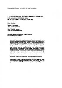
In previous literature (King et al. 1995), without special preprocessing, the testing error rates acquired by using other pattern classification methods are reported, such as 16.3% from logistic discrimination, 15.5% from quadratic discrimination, 12.1% from RBF neural networks and 9.4% from k-nearest-neighbor method and so on. The complete description can be referred to (King et al. 1995). To confirm the validity of the multiclass SVM algorithm proposed in this article, the decision tree needs to be constructed for dividing the training datasets firstly. The Gaussian radial basis function kernel with parameter r ¼ 64 was chosen as the kernel function for every node in the binary tree, and then performing the algorithm addressed in last
Figure 2. Binary tree constructed by using Landsat satellite image datasets.
200
Z. LU ET AL.
Downloaded By: [Brown University] At: 04:47 3 April 2007
Table 2. Comparison on error rates of different multiclass SVM algorithms on the Landsat satellite image testing datasets Multiclass SVM algorithm Testing error rate
One-to-others
Pairwise
All-in-one
Method in this article
9.65%
9.20%
9.15%
9.05%
section yields the topological structure of binary decision tree as shown in Figure 2. After determining the structure of the decision tree, the training for the multiclass SVM can be executed. In our experiment, the soft margin SVM with C ¼ 2 was trained in every nonleaf node by using the training datasets without any special preprocessing. Next, we calculated the test error rate on the testing datasets, and compared with those obtained from conventional multiclass SVMs, where the exactly same kernel and parameters were adopted. The results were listed in Table 2. In general, the multiclass SVM algorithms achieve higher accuracy than other pattern classification methods used in (King et al. 1995). On the other hand, at the lower cost of computational complexity in both phases of training and testing as discussed in the first section, the decision tree based SVM algorithm proposed in this article outperforms the conventional multiclass SVM algorithms in terms of accuracy.
CONCLUSION An innovative method of designing the structure of decision tree for multiclass SVM to improve its performance in both computational complexity and classification accuracy was presented in this study and concurrently the problem of unclassified region was overcome. Based on a new kernel-induced distance function, it is from the perspective of dissimilarity between classes in the feature space that the kernelized hierarchical clustering was developed and used in designing the decision tree. Simulation results on Landsat satellite image dataset support our findings. In the future work, we will delve into the theoretical underpinning of the distance function used in our method in more detail and extend it to more classification and recognition tasks.
MULTICLASS SUPPORT VECTOR MACHINES
201
Downloaded By: [Brown University] At: 04:47 3 April 2007
REFERENCES Abe, S. 2005. Support vector machines for pattern classification. London: Springer Verlag. Baudat, G. and F. Anouar. 2000. Generalized discriminant analysis using a kernel approach. Neural Computation, 12:2385–2404. Cheong, S., S. H. Oh, and S. Y. Lee. 2004. Support vector machines with binary tree architecture for multi-class classification. Neural Information Processing – Letters and Reviews, 2(3):47–51. Cristianini, N. and J. Shawe-Taylor. 2000. An introduction to support vector machines and other kernel-based learning methods. Cambridge, UK: Cambridge University Press. Eiter, T. and H. Mannila. 1997. Distance measures for point sets and their computation. Acta Informatica, 34:109–133. Franc, V. and V. Hlavac. 2004. Statistical pattern recognition toolbox for MATLAB. Prague, Czech: Center for Machine Perception, Czech Technical University. Girolami, M. 2002. Mercer kernel-based clustering in feature space. IEEE Tranactions. on Neural Networks, 13(3):780–784. Hsu, C. W. and C. J. Lin. 2002. A comparison of methods for multiclass support vector machines. IEEE Transactions on Neural Networks, 13(2):415–425. King, R., C. Feng, and A. Shutherland. 1995. Statlog: Comparison of classification algorithms on large real-world problems. Applied Artificial Intelligence, 9:289–333. Mu¨ller, K. R., S. Mika, G. Ratsch, K. Tsuda, and B. Scho¨lkopf. 2001. An introduction to kernel-based learning algorithms. IEEE Transactions on Neural Networks, 12(2):181–202. Pekalsak, E., P. Paclik, and R. P. W. Duin. 2001. A generalized kernel approach to dissimilarity-based classification. Journal of Machine Learning Research, 2:175–211. Roth, V. and V. Steinhage. 1999. Nonlinear discriminant analysis using kernel functions. In Advances in neural information processing systems 12, edited by S. A. Solla, T. K. Leen, and K.-R. Mu¨ller. Cambridge, MA: MIT Press, pp. 568–574. Scho¨lkopf, B. 2001. The kernel trick for distances In Advances in neural information processing systems 13, edited by T. K. Leen, T. G. Diettrich, and V. Tresp. Cambridge, MA: MIT Press, pp. 301–307. Scho¨lkopf, B. and A. J. Smola. 2002. Learning with kernels: Support vector machines, regularization, optimization, and beyond. Cambridge, MA: MIT Press. Scho¨lkopf, B., A. Smola, and K. R. Mu¨ller. 1998. Nonlinear component analysis as a kernel eigenvalue problem. Neural Computation, 10(5):1299–1319.
Downloaded By: [Brown University] At: 04:47 3 April 2007
202
Z. LU ET AL.
Theodoridis, S. and K. Koutroumbas. 1998. Pattern recognition. San Diego, CA: Academic Press. Vapnik, V. N. 1998. Statistical learning theory. New York: John Wiley & Sons. Webb, A. R. 2002. Statistical pattern recognition. England: John Wiley & Sons. Weston, J. and C. Watkins. 1999. Support vector machines for multi-class pattern recognition. In Proceedings of the 7th European Symposium on Artificial Neural Networks, Bruges, Belgium. Zhang, D. Q. and S. C. Chen. 2004. A novel kernelized fuzzy C-means algorithm with application in medical image segmentation. Artificial Intelligence in Medicine, 32:37–50.