Design of neural networks model for transmission ... - Springer Link

Journal of Mechanical Science and Technology ( KSME Int. J.), Vol. 19, No. 10, pp. 1873--1884, 2005 1875

Design of Neural Networks Model for Transmission Angle of a Modified Mechanism ~ahin Yddlnm*, Selquk Erkaya, Siikrii Su, Ibrahim Uzmay Erciyes University, Engineering Faculty, Department o f Mechanical Engineering Kayseri / TUR K E Y

This paper discusses Neural Networks as predictor for analyzing of transmission angle of slider-crank mechanism. There are different types of neural network algorithms obtained by using chain rules. The neural network is a feedforward neural network. On the other hand, the slider-crank mechanism is a modified mechanism by using an additional link between connecting rod and crank pin. Through extensive simulations, these neural network models are shown to be effective for prediction and analyzing of a modified slider-crank mechanism's transmission angle.

Key Words : Transmission Angle, Neural Network, Slider-crank Mechanism, Learning Algorithms

Nomenclature TDC BDC tl

rc l r~ e 0 q~i q (.)

ydi yi O w r/ a &" b~ -t

: Top dead center : Bottom dead center : Transmission angle : Crank arm length : Connecting rod length : Radius of pinion gear : Distance of eccentricity : Crank rotation angle : Weighted sum : Non-linear dynamic function : i th desired outputs : t~h outputs of the network : Unknown parameters : Network weight : Learning rate : Momentum constant " Error signal of the i TM neuron in the rn th layer " Bias input to neuron i in layer m - - I .

* Corresponding Author, E-mail : sahiny@ erciyes.edu+tr Erciyes University, Engineering Faculty, Department of Mechanical Engineering Kayseri/TURKEY. (Manuscript Reeeived December 8, 2004; Revised August 18. 2005)

ni nj n~ N RMSE

: : : : :

Number of neurons Number of neurons Number of neurons Training numbers Root Mean Square

in the input layer in the hidden layer in the output layer Error

I. Introduction There has been considerable interest in the past few years in exploring the applications of artificial neural networks (ANNs) for analyzing and prediction mechanisms. Also, modeling applications of neural networks received increasing attention due to their versatility, such as non-linear mapping, linear adaptability and parallel processing. A neural network has been employed as a case-based approach for analyzing dimensions of a planar linkage (Vasiliu and Yannou, 2001). In addition to neural network approach, various classical method schemes have been studied to achieve good tracking performance of the slidercrank mechanism. Soylemez has analyzed slidercrank mechanism using complex algebra method (S5ytemez, 2002). The complex algebra has employed to solve classical problem. The solution was obtained as the root of cubic equation within

1876

v~ahin Yd&r#n, Selquk Erka.va, ~tikrii Su and lbrah#~ 65may

a defined range. Shrin[vas and Satish have proposed importance of the transmission angle for most effective force transmission. In their paper, 4, 5, 6 and 7 bar linkages of the mechanisms were investigated (SErinivas and Sa:ish, 2002). Kim and Jung have investigated the theoretical mechanism for driving the tapered pistons by using of che geometric method (Kirn and Jung, 2003). In their research, the driving area of the tapered pistons was analyzed by measuring the strain of a cylinder forced against a tapered piston using an electric strain gauge and a slip ring. The forces applied to tapered pistons were also investigated wfih the change of discharge pressure and the rotational speed. Atria has analyzed a numerical algorithm for kinematic analysis of a multi-Iink five-point suspension mechanism (Atria, 2003). In his paper, geometric constraints for the system were introduced to fix the relative positions between the points belonging to the same rigid body. Position, velocity and acceleration analyses were carried out and the presented results were discussed. Choi has also investigated kinematic analysLs and optimal desig~ of a 3-PPR planar parallel manipulator, which consisted of three active prismatic joints, three passive prismatic joints, and three passive rotational joints (Cho[, 2003), In his research, [or the kinematic analysis, direct and inverse kinematics, and inverse Jacobian of the manipulator were derived. Also, for the optimal design of the manipulator, an optimal design procedure was carried out using Min-Max theory. Lee et al. have investigated a constraint operator tbr the kinematic calibration of a parallel mechanism (Lee et al., 2003). They constrained the movement between two poses by adopting the concept of a constraint operator. Also, a cost function was derived by the errors between the theoretical movemen~ and the actual movement. FinalIy, the parameters that minimize the cost function were estimated and substituted into the kinematic model for a kinematic calibration. The paper is organized in the foLlowing manher, Section 2 describes the theory of transmission angle of the modfl'ied slider crank mechanism. Some details of :he neural networks and learning

algorithms are outlined in section 3. Simulation results are given in section 4 and the paper is concluded within section 5.

2. Modified Slider-crank M e c h a n i s m Modified slider--crank mechanism, as shown in Fig, 1, has an additional extra link between

~ ~ 3.....

O

~ ~ " JLr'".l

"

...-.6

"

"

O Rototion cemer of the crank shaft A Crank-pill center C Piston pin center l Crank shaft bearing 2 Crank arm 3 Eccentric connector 4 Connecting rod 5 Piston 6 7 8 9 : Elemcnt~ of the cpicyclic gear mechanism Is~ transmission line : 4-3-2 2nd transmission [me : 4-3-6-7-8-9-2 Fig. 1 Schematic represent,'ttion of the modified slider crank mechvnism

Design of Neura~t Net~rks ModeI.for TransmisSiOn Angle of a .M~diJTedMechanism connecting rod and crank pin as distinct from well-known slider-crank mechanism. The new extra link may be called eccentric Connector and transmits gas forces to the crank and also drives a plan.eta~ gear mechanism. In order to d r i ~ planetary gear train, a pinion fixed to the eccentric conne~tor in a paraUei plane is used. So, there are two transmission lines in this new system, One of them eal!ed direct transmission line consists of eontaecting rod-eccentric c0nnect.mrcrank arm and the other called indirect transmission line consists :of connecting rod-eccentric connector-gear mechanism. When the motion characteristic of the mechanism in Fig, i is outlined. carefully, a kinematicbased scheme in Fig. 2 is obtained. Referring to Fig. 2, i.t 6a:n .be ,m~n that the modified mechanism has. one degree ~f freedom, that is, this model is a ~onstrained .mechanism. The eccentric .conneetor has a eurvilincar translation because of the particula~ :choice o.f gear ratio

+.

,'"

II..

:i/ ~

,

,I

;

'

%t~ "/

x

k.t-

" '

,4,

;

'

-I--

J,- -~,-.

I

~,.

,

.

q"

#-

!

% \

I

~ ----j ,,,

I [-

~

-r

/

.

-

-

s,

-

/

I P

Eig, 2 Working scheme of the modified mechanism on X¥ ptane

Table I

1877

Kinemad¢ parameters: 0fthe modified m~hanism

P.arametexs

Values (ram)

•re

50 2~9

•

r~

5O

e

35 ~ 65

between pinion a.nd ring gear. St>, it has no. a relative motion with respect to crank pin. The kinematic parameters and values of the modified mechanism are given in Table 1. 2.1

T r a n s m i s S i o n a n g l e of m ~ e h a n i s m

The transmission ~tngiv (t.t) is an important eriteri'on for design of the mechanisms, which denotes the quality of motion ~ansmission in a mechanism. It helps, to. decide the "BesC among a family o.f possible meckanisms for most Offee.tire force transmission ,(Shrinivas and Satish, 2002). U~ually, traasmission angle iS used to obtain better results for vario~.s linkage app.lica: tions. The mechanism designed with cosine of :maximum transmission angle criterion will have minimum force acting along .the coupler and on the be.arings. Although agood transmjssian annie is not a cure-all for every design problem, for many mechanical applieati0ns it earn guarantee for the performance of linkage at higher speed without unfavorable vibrations. When /z=90 ~, most effe~eti.veforce transmission: takes piaee and the accuracy of output motion is less sensitive to manufacturing tol~.ances of link lengths and ¢learance between joints and change of dimensions due to thermal expartsion~ Meeh~nisms having transmissi:on angle too much deviated from 90~, ex.hiSit poor operational characteristics like noise and jerk. at high speed~. If ,u~0 °, self-tockigg takes pl.aee; Transmission angel in a mechanism provides a very good of the quality of motio~ expected no~se output .and its. costs in general. In other words,, it is a simple, and u~eful coefficient of perle:finance in me,ehanisms for non-uniform mO~ion transmission. The transmission .angte does not consider the dyn.amie forces due to velocity and acceleration.

~ahin rddmm, ~e!~k grkaya, ~kr~ Su and tbmhtm Uzmay

i878

aJ .~" m. •

.'.,

• • . ~ }

./, '%

" ,I

I

-

. ,

' "~ " ' -% "" .% ~

I b:i;-:::i.:

%%. " ' " %

,

•

II

'%"

,"--' ..". ?-.

1I.

. ....

~t

;0

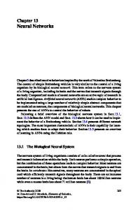
Ng. 3 The tr.ansmissi~n a.n#e varimi.ons of the modified system ~ecaus:e of this reason, it is widely u s ~ i.n kinematic ~synthesis .stage duri:ng which the lengths and mass properties ..of the tlnk~ are unknown. K~nematieally expregsed transmission angle .dnes not reflect theaeti0n of gravity or dynamic forees. 80, for the determination of transmission characteristics of the linkage, it is not neCeSsary to analyze the forces and torque acting at each joint of the Whole meehanism. Referring to Fig. 2, the transmission -angle equation for the modified mechanism can be..described as~; l ¢ ~ tz=r¢.sin O.+r~,- e

(1)

.,a=:c~s_~( r,..sin 8+.e~- e l )

(::~)

From Eq. ~2~, th.o transmission .~ugi~ depends on mainly two variables : :eccentricity ~alu~: and crank rotation angle..that i~,/z=f.(~., e~. The other parameter~ ; re., r~ and ../.are.co.nstant terms. The relationship between eccentricity value, and transmission angle during one cycle is outlined .in

Fig.,

3.

3.

Feedforward

Neural

Network:

The arohiteeture of the neural network is ;shown in Figure .4. The structure i.s the same as.a feed-forward ANN except for the learning algorithms. As it can be seen from Figure 4, neural network eo~sists of three layerg, which are input, hidcten a-rid output layers. The input tayer with

O

x~,~ rll k'-J' "!.'~,q,*r

] ~nea, n e u l ~ r "

•e : ~eeentriefty .value of me¢hanism n~ : Numl~er ofneurons in: the inpt~t layer (~= i) n~ : Numbe~'.ofueurons in the hldde_n.layer (j=l, .,-, tO) n~ : Number of neurons in the Output layer ~k=l, ...,. 37) Fig, 4 A Feedfor~ard NN for kinematic analysis of modified mechanism one neuron, the hidden layer with i0 neurons a~ad the output layer with 3.7 ttcumus are emp!~yed ~s a predictor o f ~he m~chanism. The network .architecture is defined by the basic pr0eessing etement8 and the way in which they are imer¢:o:nneeted. The :basic pr0ee.s~ing element of the e0nneerionizt architecture, is often a i l e d .a u~uro.n by analogy with neuroph~siology. Many of the basic processing elements may be .considered to have three components; ( ~ A weighted sumea(2) A linear dynamic single in~pnt.single .Output (S~SO~ (3) A non-tin.ear d y ~ m i e funetiorl These elements are considered in turn in the following section. The. weig.hted .~umer is describedby N

M

q~,.(t):~a.e-y,.(t) =~b~u~(t.)=. +w,

(3)

giving a weighted :sum q~; in terms of the outpu~ :of all elements y~., external inputs -u, a.nd corresponding weights a~ a~d b~ together with constants w~-.N of these ~veighted sumer elements

Design of Neural Networks Model for Transmission Angle of a Modified Mechanism can be conveniently expressed in vector-matrix notation. Stacking N weighted sums ~ into a column vector p, the N outputs ye into a vector y and M inputs u~ into a vector u and the N constants w~ into a vector w, equation (3) may be rewritten in vector matrix form as : g,(t) = A y (t) + B u (t) + w

(4)

where the ij ~ element of the N X N matrix A is and the element of the N X M matrix B is b~,. The constants w~ could be incorporated with the inputs u~, but it is useful to represent them explicitly. The linear dynamic SISO system has input cp and output x¢. In transfer function form, it is described by

x~(s) = H ( s ) ~o,(s)

a]

c7

_ ~l

0 W,~

Oy,

(10)

~y, a W,7

From equation (8) OJ_ ~y~

( y a , _ y , ) = _ e~

(11)

where ~ is called the error signal of the i th neuron in the TK~th layer. From Equation (10)

(5) Oy, 0 WiY

xr_t

(12)

Thus, (6)

31

where H ( s ) and h(t) form are a Laplace transform pair. The non-linear dynamic function g ( . ) gives the element output y, in terms of the transfer function output x~:

y,=g(x,)

(9)

Although the one-hidden layer model is used in the present application, it is useful to derive the gradient of ] for the general case, and the result for the one-hidden-layer model can readily be obtained as a special case. Starting from the output layer m of the network and setting 0~= W~', the application of the chain rule gives rise to

In the time domain ; above equation becomes :

x,(t) =f[h(t-t')~,(t')dr"

1879

(7)

OW,7

-

3,'x7

'

(t3)

Next consider the ( m - - I)th layer. Using the chain rule yields : ~.~

no

m- 1

- ' ~ ~] x Oy~ × Ox~'-~ OW.,.7-~ ~-~ Oy, 3xT -~ Oz'p-1

×

~z~ -~ 3W,~ -~ (I4)

Then

3.1 Learning algorithms The learning algorithm topology, which was employed for the neural network updating the weight can be described as follows; define the error function as (Canbulut et al., 2004)

J=~(yd,(t)

-y,(t) )2

(8)

where y d i ( t ) are the i TM desired outputs and y i ( t ) are the i TM outputs of the network. This error function is to be minimized with respect to all the unknown parameters q). In the steepest descent approach the parameter vector ~ = [ 0 L , 8z, "', On]T is adjusted using the increment vector [A01, Ate, ..., AOn] ~ defined along the negative gradient direction of J

and

9 ~ . 7 -1

g'(z) =

o~g(z)

~2-

(17)

and g(zi) is the activation of neuron i. By defining the error signal for the i th neuron of the ( m - - 1) th layer as : ~tO

8?-'=g'(z';-') k~= l at w~'~

(18)

Equation (8) can be rewritten a s : aJ

0 W~-'

_

~?_]xp_2

(19)

~880

~akin Ytldtnm, Sel q:utt Erkaya, ~;~tkrft Su and i brahim Uzmay

Sim.ilarly it can be .shown that

aJ _ _ ~_~

networks according tO

(20~

w ~ t l =w,~ ( t - 1) +A w#.(t.)

(27)

b/~(t). = b~ ( t - r9 +/xb~'(.t)

(2~)

and where b~ -j is the bias i.nput to neuron .:i in layer m--r. By c:~rrying on this procedure, Eqt~ations (18) (20) can be .used as a general algorithm for updating weights in o:ther layers. Equations (i8):-(20I indicate how the error Si~als propagate backwards from the output Iay~r af the net~ork ~hrough tb.Chj.dd.~n: ta~er to the input [a.yer, hence the name '"BP'. The steepestdescent minimization of theerror funct[ondefined in Equation (8) produe~ the following inere, ments: for updating..@ : A W~: (t) ~w.d~'(tlXY'~(t)

(21)

where the increments AW~ (t) and Abe(t) are: given in equations in (25) and (26). The neural network was trained and tested by using, five types, o f Iearning algorithms: The algorithms can be described in the following forms.

Onlfne-haekpropagation algorithm (Case 1)

3,1.I

Online Backp.ropagation which updates the 'weights after each .pattern is presented to the network. Back-propagation is the most commonly used training, algorithm for neural networks. The weights: are .updated as fOllOWS

where in .the output Ia)~er

, ~ (t) =y~, (t) -y,~:t)

:(~3)

and in ~ther layers.

b P, •

p

•

.

-

i • .

.

..

..

. -

.

, b

:2

The¢onstants ~.~ ( 0 < ~ . < 1 ) and ~1~ ( 0 < ~ < 1 ) represent the ~earning rates: for the weights and biases respeeti~eiy: In praefiee, a large value of the learning rate wo:~aldbe preferable, because this would result in ~:pid Iearniag. Unfortunately, a large vaIue of the }earning rate Can .also }cad to oscillation or even .divergen.e~. To help. speed up learning bm ~ i d undue., ose:ilM~ion~,:a momenturn term is usu.ally included so that Equations (2I) and .(22) become

v~here a~and a~ are momentum constants, which determine the effect of past changes of ~ (t) and Abp (~) oz the' current updating direction in the weight and the. b~as: space respeetb~ely. This effeetiveIy filters o:ut high frequency variations in the error surface. To summarize, the BP algorithm updates the weights and thresholds, of the.

-

,

• • •

• "-i.

~ " t

p . . . .

~

•

. •

•

....

, .

".

%~,~,s

" . . ,

, ..

,

,, •

, r

~ - ~ .

4

,

Fig. fi(a) The actual trartsmiss[on ag~g!evariations uNng ~nl:ine BP Iearning algorithm

° -z,

. ,h

•

a~J 1

.I

Fig. s (b)

The RM8Es using .online BP .learning algorithm

Design of. Neurat Ne¢~orks Model for. Transmission. Angle of a Modified MeehaMsm

Aw;~(t) = - ~ ~gW.,~:(t) t-:~~¢~t-li

(29)

where r) is the. learning rate, and a is the momentum constant. The actual results for "Oflline Baekpropagation Learning Algorithm" can be outlined in .F(g. 5(a)i. From Fig~ 3 and Fig., 5 (a), th~ deviations between •desired and •actual res:ults. (RMS Error) using Online BP Learning Algorit.hra is shown

:in Fig. 5.(h). 3.L2 Batch backpropagation algorithm

(Case 2): Bateh Backpropagati0n with weight update~ occurring, after each epoch. The: actual results for "Batch Backp.ropagati0n Learning Algorithm" can be outfined in Fig. 6 ~a).

1881

From Fig, 3 and Fig. 6(a)., the deviations between desired :and actual results using B_ateh BP Learning Algorithm. is s~ovcn in Flg. 6 (b).. 3,1.3 Delta-Bar-Delta algorithm (Case 3) DeIm-.Bar-Delta is a.n adaptive learning rate method in which every weig!lt has. its own learning rate. The learning rates .are updated, hasexl on th¢ sign .of the gradient. !f the gradient does not chala.ge ~gns on successNe iterations then the step size. is increased Hnearly. If th~ gradient changes. signs; the learning rate is de.er,ased exponentially. tn some eases this method seems to learn much faste~ than non-adaptive methods,. Learning rates, 7](.t) are ,u~dated as follows: K

A~ (t) =

.if ~"(.t-

Ill) ~ ' ( t ) : > 0

- : ¢ , l (~) ~f ~ : ( t - l) ~ (t) < 0 O: e/se

(~o)

4,v,~

ii!iii!iiii!!iii!!! • -, ",: ii iii iiiiii,iiiiiiiiiiiiii!!i!i!? ~

4, ,

i

•

I

I

•, . , . . , . % .

,

~..

",.'i

"=~..'-,:'. "..'....,

~

lib

Fig. 6~a)

The actual tmn.smissio~ angle v~nations using .batch BP learning algorithm

Fig, 7(a)

The actual transmission .angle variations U~ing delta-bat-delta learning aigorffhm

'!

t. ,! •J .3 $ ,)q. .b' t'fct

1

-" 11,

tt -

"7'.

T

Fig, 6 (b) The RMSEs u~-ingbatch BP learning algorithm

at¢

¢" ~ .. ~b ~ . -

4

The RMSF~. u~ng delta-bar-delta learning aIgorifl:tm

.re,ahin Yddtnra, Selquk Erkay~ ~kr~l Su and ibrahim Uzmay

1882:

where d ( t ~ ) =OE ~ at time t arm ~- is the exponentlal average of past values of d.

~-(~) = (1- al ~(t:) +.a~-~t- !)

(31)

The actual resul.ts for "Dolt.a-Bar-Delta Learning Algorithm" can be outlined in Fig.. 7(a)÷ From Fig; 3 an:d Fig. 7~a), the deviations, between desired and ,actual results using.. DehaBar-Delta Learning Algorithm is shown in Fig. 7

(h) 3+1,4

Random

baekpropagation

their .magnitudes. Each weight, w~:~,has its own step :size or update value, Ai¢ which varie~ with time t according to : if~E . i ~ ~E,t~

hz(t) = / ~.-.6o(t-l), if~(t-1).~(~).