Design of Wireless Power Transfer System via Magnetic Resonant Coupling at 13.56MHz Ajay Kumar Sah Department of Electronics and Computer Engineering, IOE, Central Campus, Pulchowk, Tribhuvan University, Nepal
[email protected] Abstract: Power is a must to modern systems. Power transmission through wires is common. But not in every field can wires be used because of certain limitations. The implantable biomedical devices like pacemakers, cardiac defibrillators, and artificial hearts require power supply for long term operation. The required power is supplied by driveline cable or by battery. WPT greatly reduces the risk of infection by eliminating the driveline cable which otherwise needs to puncture the skin to provide power and also saves the valuable space inside a person’s body in case of battery powered. In such fields, what we need is wireless transmission. Wireless transmission is useful in cases where instantaneous or continuous energy transfer is needed, but interconnecting wires are inconvenient, hazardous, or impossible. In this paper, a simple design method of a wireless power transfer system using 13.56 MHz ISM band is proposed. The proposed wireless power transfer system consists of rectifier, oscillator, power amplifier, power coil, load coil and two intermediate coils as transmitter antenna and receiver antenna inserted between power coil and load coil. Keywords: Wireless Power Transfer, Resonant coupling, Oscillator, Intermediate coils, Power transfer efficiency.
1. INTRODUCTION Power is very important to modern systems. From the smallest sensors, bionic implants, laptops, consumer products to satellites and oil platforms, it is important to be able to deliver power means other than classical wires or transmission lines. Wireless transmission is useful in cases where instantaneous or continuous energy transfer is needed, but interconnecting wires are inconvenient, hazardous, or impossible sometimes. In case of biological implants, there must be a battery or an energy storage element present that can receive and hold energy. This element takes up valuable space inside a person’s body. In case of satellites, UAVs and oil platforms, solar panels, fuel cells or combustion engines are currently used to supply power [1]. The history of wireless power transmission dates back to the late 19th century with the prediction that power could be transmitted from one point to another in free space by Maxwell in his “Treatise on Electricity and Magnetism”. Heinrich Rudolf Hertz performed experimental validation of Maxwell’s equation which was a monumental step in the direction. However, Nikola Tesla’s experiments are often considered as being some of the most serious demonstrations of the capability of transferring power wirelessly even with his failed attempts to send power to space [2]. There are three types of Wireless Power Transfer (WPT): radiative transfer, inductive transfer, and resonant coupling. Radiative transfer, although suitable for exchanging information, can transfer only small power (several millwatts), because a majority of energy is wasted into free space. Directive radiative transfer using highly directional antennas can be efficiently used for Proceedings of IOE Graduate Conference, Vol. 1, Nov 2013
power transfer, even for long distances, but requires existence of an uninterruptible line-of-sight and has harmful influences on human body. On the other hand, inductive coupling can transfer power with very high efficiency but in a very short range (just in several centimetres) [2]. The last type of WPT, resonant coupling, can transfer high power at the medium range (several meters). Recently, MIT proposed a new scheme based on strongly coupled magnetic resonances, thus presenting a potential breakthrough for a midrange wireless energy transfer. The fundamental principle is that resonant objects exchange energy efficiently, while non-resonant objects do not. The scheme is carried with a power transfer of 60 W and has RF-to-RF coupling efficiency of 40% for a distance of 2 m, which is more than three times the coil’s diameter. We expect that coupled magnetic resonances will make possible the commercialization of a midrange wireless power transfer [3]-[5].
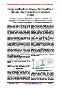
2. RELATED THEORY A. Resonant frequency Resonance is a phenomenon that causes an object to vibrate when energy of a certain frequency is applied. In physics, resonance is the tendency of a system (usually a linear system) to oscillate with larger amplitude at some frequencies than at others. These are known as the system’s resonant frequencies. In these particular frequencies, small periodic driving forces can even produce oscillations having large amplitude. The resonant frequency is calculated from (1).
202
receiver would be more difficult to tune, but would have more selectivity. In an ideal series RLC circuit and in a tuned radio frequency receiver (TRF) the Q factor can be written as shown in (2). (2) Where, R, L and C are respectively the resistance, inductance and capacitance of the tuned circuit.
C. Necessity of Impedance Matching Figure 1: Resonant frequency
(1) Where, L and C are respectively the inductance and capacitance of the tuned circuit.
B. Quality Factor (Q) In physics and engineering the Quality factor (Q-factor) is a dimensionless parameter that describes the characteristics of an oscillator or a resonator, or equivalently, characterizes a resonator’s bandwidth relative to its centre frequency [1]. Higher Q indicates the stored energy of the oscillator is relative of a lower rate of energy loss and the oscillations die out more slowly. So it can be stated that, oscillators with high quality factors have low damping so that a pendulum rings longer, in case of a pendulum example.
The resonance frequency changes as the coupling factor changes, and the maximum efficiency power transfer occurs at the resonance frequency. However, when this wireless power transfer system is applied in the MHz range (which allows smaller antennas), the usable frequency range is bounded by the Industrial-ScientificMedical(ISM) band as shown in Figure 3. According to the ISM band, the usable frequency ranges are extremely narrow. For example, at 13.56MHz, the usable frequency range is 13.56MHz±7kHz [6].
Figure 3: ISM Band
As a result, to apply this technology in restricted frequency ranges such as the MHz range, the frequency of the power source must be fixed at a usable range, and the system has to be tuned so that its resonance frequency matches the frequency of the power source.
D. Basic Theory of Impedance Matching Figure 2: Bandwidth versus frequency
The above graph is the representation of the bandwidth, Δf, of a damped oscillator energy versus frequency. The higher the Q, the narrower and ‘sharper’ the peak is foΔf. Sinusoidal signal driven resonators having higher Q factors resonate with greater amplitudes (at the resonant frequency) but have a smaller range of frequencies around that frequency for which they resonate; the range of frequencies for which the oscillator resonates is called the bandwidth. Thus, a high Q tuned circuit in a radio
Proceedings of IOE Graduate Conference, Vol. 1, Nov 2013
Impedance Matching is a technique commonly used in power transfer systems and communication systems to improve the efficiency of the system. It usually involves inserting a matching network (such as an LC circuit) to minimize the power reflection ratio to the power source of the system. In Figure 4, the power transferred to the load is written as (3) when the impedance of the power source is defined as Zsource and that of the load is defined as Zload. The power transferred to the load reaches its maximum when Zsource=Z*load, as in (4). Therefore, the circuit is considered matched and the maximum efficiency achieved when the impedance of the load from
203
the source's point of view matches Zsource, and vice versa [1].
Figure 4: Theory of impedance matching
(3) (4) The Impedance matching circuit can be considered as a two-port network that can be described with (5). The matching conditions are satisfied when the parameters satisfy (6) & (7). (5) (6) (7)
E. Equivalent Circuit diagram of the WPT System
Figure 5: Equivalent circuit of WPT system
Figure 5 shows the circuit representation of the WPT system as modelled above. The schematic is composed of four resonant circuits corresponding to the four coils. These coils are connected together via a magnetic field, characterized by coupling coefficients k12, k23, and k34. Because the strengths of cross couplings between the power & Rx coils and the load & Tx coils are very weak, they can be neglected in the following analysis. Theoretically, the coupling coefficient (also called coupling factor) has a range from 0 to 1. If all magnetic flux generated from a transmitting coil is able to reach a receiving coil, the coupling coefficient would be “1”. On the contrary, the coefficient would be represented as “0” Proceedings of IOE Graduate Conference, Vol. 1, Nov 2013
when there is no interaction between them. Actually, there are some factors identifying the coupling coefficient. It is effectively determined by the distance between the coils and their relative sizes. It is additionally determined by shapes of the coils and orientation (angle) between them. The coupling coefficient can be calculated by using a given formula (8) Where M12 is mutual inductance between coil “1” and coil “2” and note that 0 ≤ k12 ≤ 1. Referring to the circuit schematic, an AC power source with output impedance of Rs provides energy for the system via the power coil. Normally, the AC power supply can be a power amplifier which is useful to measure a transmission and reflection ratio of the system. Hence, a typical value of Rs, known as the output impedance of the power amplifier is 50 Ω. The power coil can be modelled as an inductor L1 with a parasitic resistor R1. A capacitor C1 is added to make the power coil resonate at the desirable frequency. The Tx coil is a helical coil with many turns represented as an inductor L2 with parasitic resistance R2. Geometry of the Tx coil determines its parasitic capacitance such as stray capacitance, which is represented as C2. Since this kind of capacitance is difficult to be accurately predicted, for fixed size of the coil, a physical length, which impacts the self inductance and the parasitic capacitance, has been manually adjusted in order to fit the resonant frequency as desired. In the receiver side, the Rx coil is modelled respectively by L3, R3 and C3. The load coil and the connected load are also performed by L4, R4 and RL. A capacitor C4 also has the same role as C1, so that the resonant frequency of the load coil is defined. When the frequency of sinusoidal voltage source VS is equal to the self-resonant frequency of the resonators, their impedances are at least. In other words, currents of the coils would be at their most and energy can be delivered mostly to the receiving coil. Otherwise, energy of the transmitting power source would be dissipated in the power coil circuit itself, resulting in the very low efficiency. In general, setting the frequency of AC supply source same as the natural resonant frequency of the transceiver coils is one of the key points to achieve a higher performance of the system. The circuit model offers a convenient way to systematically analyze the characteristic of the system. By applying circuit theory Kirchhoff‘s Voltage Law (KVL) to this system, with the currents in each resonant circuit chosen as illustrated in Figure 5, a relationship between currents through each coil and the voltage applied to the power coil can be captured. The system model can be considered as a two-port network. To analyze this kind of system, S – parameter is a suitable candidate. Actually, S21 is a vector referring to a ratio of signal exiting at an output port to a signal incident at an input port. This parameter is really
204
important because a power gain, the critical factor determining of power transfer efficiency, is given by [|S21|*|S21|], the squared magnitude of S21. The parameter of S21 is calculated by (9) [7]. (9) Thus, combining with derived from (8), the S21 parameter is given as
(15) It is clear that |S21|max un-proportionally depends on * k23. It means for the sake of a higher efficiency, the extent that the highest efficiency can be achievable is shortened. In order to get a greater value of |S21|max, * k23 is supposed to decrease. From (14), increasing Q2 and Q3 is able to reduce the * k23. In general, making the very high-Q transmitting and receiving coils is very crucial so as to achieve high transfer performance.
(10)
F. Wheeler's formula The system equation indicated in (10) is expanded in terms of quality factor which appreciates how well the resonator can oscillate. The quality factor is presented in a formula as given below
The classic formula for single-layer inductance (air core) is called Wheeler's formula is given as:
(11) Where i and Ri are respectively the self-resonant frequency and equivalent resistance of each resonant circuit. In the power coil, for instance, Ri is a sum of RS and R1. Actually, i of each coil is defined to be the same. When the resonance takes place, the total impedance of each coil is presented as following
Figure 6 Coil antenna
(16) Where,
Z1 = RS + R1 ≈ RS, Z2 = R2, Z3 = R3,
L = inductance in micro-Henries
Z1 = RL + R4 ≈ RL
N = number of turns of wire
For simplicity, it is common to set RS equal to RL. At the resonant frequency, 0 = 1 / LiCi, from (10), the magnitude of S21 can be written as (12)
R = radius of coil in cm H = height of coil in cm
3. WPT SYSTEM DESIGN CALCULATIONS A. Block Diagram of Proposed System
The coupling coefficient k12 and k34 would be constant. There is only k23 varying with medium conditions. To find the range between the resonators at which |S21| or the efficiency is certainly at maximum, a derivative of S21 with respect to k23 is taken and then setting the result to zero, yielding (13)
The paper will be based on the principle of resonant inductive coupling. Magnetic coupling is an old and well understood method in the field of wireless power transfer. But as magnetic fields decay very quickly, it’s effective only at a very short distance. By applying resonance within magnetic coupling, the power transfer at a greater distance can be obtained. For near field wireless power transfer, Magnetic resonant coupling can be more effective than any other methods available. The structure of the whole system is shown below.
(14) This value of * k23 is equivalent to the maximum range that the transmitter is able to effectively transfer power to the receiver at the given resonant frequency (before the resonant frequency breaking in two peaks). Note that * k23 ≤ 1. With the purpose of finding out the maximum efficiency of the system in terms of |S21|, it is feasible to substitute k23, which is derived above, into (13) Figure 7: Structure of the WPT System
Proceedings of IOE Graduate Conference, Vol. 1, Nov 2013
205
Here, I assume: Object A represents high frequency oscillator. Object B is representative of signal amplifier.
smaller reservoir or smoothing capacitor than an equivalent half-wave rectifier. The full-wave bridge rectifier is designed on the Cadence, PSPICE Simulator as shown in Figure 9 and the result is shown in Figure 10.
Object C is a source coil. Object F is a load coil. Object G is a resistive load. Object D and E are transmitter and receiver antenna respectively. By including a signal amplifier in the system, it will be able to amplify the amount of power that is transmitted. This is crucial for conduction tests at high power. From the amplifier the signal is then dumped into object C. This is located at the top of object D. This allows for the resonate frequency to pass from the object C to D. When the transmitting antenna begins to resonate it generates the evanescent resonate waves. Object E will pick up these waves. From the receiving antenna, the signal is then passed to object F. The load coil will then pass the signal on to the load G.
Figure 9: Rectifier
Figure 10: Input and Output curves of Rectifier
The following oscillator circuit is used. This oscillator uses PSPICE VPULSE that generates square wave in combination with H bridge amplifier.
Figure 8: Block Diagram of the whole system
The intermediate coils D and E are placed between object C and F, which is tuned at the same frequency as C and F. The coil D, being in the area of the magnetic field generated by coil C, receives power. Similarly, coil E, being in the area of the magnetic field generated by coil D, receives power. Not having any resistive load, the coil in turn generates its own oscillating magnetic field. The advantage of using these intermediate coils is that these coils are completely separated from the source internal resistance. This increases the Q-factor, allowing greater power to be radiated.
When MOSFET M1 and M4 are turned on we have a positive voltage, when all 4 MOSFETs are off we have 0 voltage, and when MOSFETs M2 and M3 are turned on we get what appears to be a negative voltage because of the direction the current flows. For this reason, an hbridge amplifier creates a more efficient amplifier because we get both positive and negative voltage from a single power supply. The designed h-bridge amplifier is shown in Figure 11.
The block diagram of the whole system is shown in figure 8. For the dc source, the simple full wave bridge model is used just for the simplicity of the project. At the same time the capacitor is used for smoothing the output curve. The PSPICE circuit diagram is given below. The main advantages of a full-wave bridge rectifier is that it has a smaller AC ripple value for a given load and a
Proceedings of IOE Graduate Conference, Vol. 1, Nov 2013
Figure 11: H-Bridge Amplifier
206
The transient analysis of the designed h-bridge amplifier through PSPICE simulation is done. The oscillator generates 13.56MHz frequency and can be verified with simulation result given below in Figure 12.
From (14) and (15), with the value given in Table I, quality factors, coupling coefficient and the maximum value of magnitude of S21 parameter are calculated as follows From (1),
From (3), assuming RS=RL=50 Ohm and R1=R2=R3=R4 =0.015 Ohm,
Figure 12: Output of H Bridge Amplifier
For the rectifying purpose at the receiver, the simple full wave bridge model is used.
B. Parameter Identification of Proposed System We have from (16),
Where, L = inductance in micro-Henries N = number of turns of wire
It is assumed that the distance between power coil and transmitter coil antenna is fixed, so the coupling coefficient (k12) is fixed and assumed k12= 0.1. Also it is assumed that the distance between load coil and receiver antenna is fixed, so the coupling coefficient (k34) is also fixed and assumed k34= 0.01.The varying distance is between transmitter coil antenna and receiver coil antenna, so the coupling coefficient (k23) is a varying parameter. When the distance between Tx and Rx increases, the coupling between them decreases. From (14), the coupling coefficient is calculated as,
R = radius of coil in cm H = height of coil in cm For Power Coil, N = 2, R = 5 cm, H = 3.3 cm, Then, L ≈ 0.5 uH
From (15), the maximum value of magnitude of S21 parameter is calculated as follows
Also we have from (1),
Power Transfer Efficiency of the WPT system is calculated as,
C = 275.518 Pf The design parameters for all the antennas are listed in the table below: Table 1: Parameters of coil antennas Coil (antenna)
N (turns)
R (cm)
H (cm)
L (uH)
F (MHz)
C (Pf)
Power
2
5
3.3
0.5
13.56
275.518
Transmitter
3
6
4.4
1.3
13.56
105.968
1.67
6
4.4
0.4
13.56
344.398
1
3.7
2
0.1
13.56
1.377nf
Receiver Load
Proceedings of IOE Graduate Conference, Vol. 1, Nov 2013
4. DESIGN VERIFICATION THROUGH SIMULATION The equivalent circuit model of whole WPT system is simulated by using an advanced design system (ADS), a popular electric automation tool in RF engineering of Agilent Technologies with the circuit setup illustrated in Figure 13.
207
It can be seen from the above plot that the S11 and S22 lie on the real axis at operating frequency 13.56 MHz. The value of input port source impedance is Zo*(0.977 – j 4.939E-4) ohms and the value of output port load impedance is Zo*(0.664 – j 3.193E-4) where Z0 =ZL=50 Ohm. The equivalent circuit model to calculate the maximum power transfer efficiency ( ) is shown in Figure 16. Figure 13: Equivalent circuit of WPT system on ADS
The parameters’ values are taken from the Table I. The radius of power coil is 5 cm, the radius of load coil is 3.7 cm, radius of transmitter and receiver coil is 6cm. The power coil has two turns, load coil has one turn, transmitter coil has three turns and receiver coil has 1.67 turns. The parameter S11 is the power reflection, which is the ratio of the receiving power at the transmitter divided by the transmitting power at the same transmitter and the S21 is the power transfer, which is the ratio of the receiving power at the receiver divided by the transmitting power at the transmitter. The result of the magnitude of S21 and S11 is obtained as shown in Figure 14.
Figure 16: Simulation setup for Power transfer efficiency
The result of power transfer efficiency of the designed WPT system is shown in Figure 17.
Figure 14: Simulation result showing │S11│ and │S21│
It can be seen from the above plot, the parameter │S21│ has maximum value 0.884 which is very much close to theoretically calculated value 0.882 at operating frequency of 13.56 MHz at a distance that corresponds to the coupling coefficient k23=0.00429. The smith chart plot of Input Reflection Coefficient (S11) and Output Reflection Coefficient (S22) is shown in Figure 15.
Figure 17: Power transfer efficiency of WPT system
The maximum power transfer efficiency of the WPT system as seen from the above result is equal to 78.176% which is very close to the theoretically calculated maximum power transfer efficiency 77.79%.The above results can be tabulated as shown in Table 2. Table II: Theoretical and simulated efficiency of WPT system Parameter
Theoretical
Simulation
Maximum Power Transfer
0.882
0.884
Power transfer efficiency
77.79%
78.18%
The value of magnitude of S21 of designed WPT System for three different coupling coefficients which is a function of distance between transmitter and receiver is Figure 15: Input and Output Reflection Coefficient
Proceedings of IOE Graduate Conference, Vol. 1, Nov 2013
208
shown in Figure 18. The coupling coefficient decreases as the distance increases or vice versa.
shown in Figure 20. The coupling coefficient decreases as the distance increases or vice versa.
B. Three Coil System The circuit setup of three coil (Power coil as transmitter antenna and load coil as receiver antenna and an intermediate coil as relay antenna at transmitter side) WPT system on ADS at a distance equivalent to coupling coefficient k=0.5 is shown in Figure 21.
Figure 18: Simulation result showing │S21│ at different k23
5. COMPARISON WITH OTHER WPT SYSTEMS The simulations in this section are based on the similar conditions as in Section IV. The parameters’ values used here are taken from Table I.
A. Traditional Two Coil System
Figure 21: Simulation setup of three coil WPT System
The result of the magnitude of S21 and S11 can be obtained as shown in Figure 22.
The circuit setup of traditional two coil (Power coil as transmitter antenna and load coil as receiver antenna) WPT system on ADS at a distance equivalent to coupling coefficient k=0.5 is shown in Figure 19.
Figure 22: Simulation result showing │S11│ and │S21│
C. Designed Vs Two Coil Vs Three Coil WPT System Figure 19: Simulation setup of two coil WPT System
The result of the magnitude of S21 and S11 can be obtained as shown in Figure 20.
The Simulation results of│S11│ and │S21│ of designed WPT System, Traditional two coil system and three coil systems at operating frequency of 13.56 MHz are shown in Figure 23 in a single plot.
Figure 23: Simulation result showing │S11│ and │S21│ of designed WPT System, Two coil system and three coil system Figure 20: Simulation result showing │S11│ and │S21│
The above results can be tabulated as shown in Table 3.
The value of magnitude of S11 and S21 of traditional 2 coil WPT System for coupling coefficient, k=0.5 which is a function of distance between transmitter and receiver is
Proceedings of IOE Graduate Conference, Vol. 1, Nov 2013
209
Table 3: Efficiency of two coil system, three coil system and designed WPT system k
│S11│
│S21│
Efficiency
Two coil system
0.5
0.929
0.367
13.46%
Three coil system
0.5
0.667
0.743
55.20%
Designed system
0.00429
0.012
0.884
78.18%
Systems
It is very clear from the above results that the advantage of the four coil system over the two coil and three coil system is a high efficiency at a greater distance (k=0.00429).
The distance at which the system has coupling coefficient 0.00429 and maximum efficiency of 78.18% can be found by designing the prototype of the system and using Vector Network Analyzer (VNA). Figure 18 clarifies that when the coupling coefficient k23 decreases, there is the frequency splitting issue which substantially reduces the system efficiency. Moreover, as k23 increases, the resonant frequency also changes from the operating frequency of 13.56 MHz. Therefore, an optimal control mechanism is needed to maintain the optimal resonant condition and to realize the maximum wireless power transfer efficiency as well.
REFERENCES
6. CONCLUSION AND FUTURE ENHANCEMENT The goal of this paper was to design a wireless power transfer system via magnetic resonant coupling at 13.56MHz. After analyzing the whole system step by step for optimization, a WPT system was designed. The designed WPT system has power transfer efficiency 78.18% at a coupling coefficient 0.00429. Simulation results showed that significant improvements in terms of power-transfer efficiency have been achieved. Simulated results are in good agreement with the theoretical models. It is described that magnetic resonant coupling can be used to deliver power wirelessly from a source coil to a load coil with two intermediate coils placed between the power (source) and load coil and with capacitors at the coil terminals providing a simple means to match resonant frequencies for the coils. This mechanism is a potentially robust means for delivering wireless power to a receiver from a power (source) coil at a fixed distance.
[1]
Sabuj Das Gupta, Md. Shahinur Islam, Kawser Md. Nuronnabi, Mohammad Sakib Hossain, Md. Zahid Hasan - Design & Implementation of Cost Effective Wireless Power Transmission Model: GOOD BYE Wires – published at: “International Journal of Scientific and Research Publications(IJSRP), Volume 2, Issue 12, December 2012 Edition” .
[2]
William C. Brown, "The history of wireless power transmission," Solar Energy, vol.56, no.1, pp. 3-21, Jan. 1996
[3]
Sanghoon Cheon, Yong-Hae Kim, Seung-Youl Kang, Myung Lae Lee, and Taehyoung Zyung “Wireless Energy Transfer System with Multiple Coils via Coupled Magnetic Resonances” ETRI Journal, Volume 34, Number 4, August 2012
[4]
Mandip Jung Sibakoti, Professor Derin Sherman and Joey Hambleton “Wireless Power Transmission Using Magnetic Resonance” Cornell College PHY312, December 2011.
[5]
Kurs, A. Karalis, R. Moffatt, J. D. Joannopoulos, P. Fisher, M. Soijacic, “Wireless Power Transfer via Strongly Coupled Magnetic Resonances”, Massachusetts Institute of Technology, 2007 Science, Vol. 317. no. 5834, pp. 83— 86, 2007.
From the Figure 18, it is clear that the magnitude of S21 is highest at operating frequency 13.56 MHz at a distance corresponding to coupling coefficient 0.00429. As the distance between transmitter and receiver increases or decreases, the value of S21 decreases. In fact, the transfer efficiency significantly decreases with distance variations between the transmitter and the receiver. So, the designed WPT System is very efficient at a fixed distance corresponding to k=0.00429 but deteriorates its efficiency at other distance that does not correspond to designed coupling coefficient.
[6]
Kawamura, Atsuo, and Tae-Woong Kim. "Proposed Equivalent Circuit and Parameter Identification Method for Electro-Magnetic Resonance Based Wireless Power Transfer.” April 2013.
[7]
Hoang, Huy, and Franklin Bien. "Maximizing Efficiency of Electromagnetic Resonance Wireless Power Transmission Systems with Adaptive Circuits."Wireless Power Transfer–Principles and Engineering Explorations: K. Y. Kim, ed., InTech, 2012. Print.
[8]
Jordan, Edward C., and K. G. Balmain. Electromagnetic Waves and Radiating Systems. Second ed. New Dehli: Prentice-Hall of India, 2006. Print.
[9]
Nilsson, James William., and Susan A. Riedel. Electric Circuits. Boston: Prentice Hall, 2011. Print.
Proceedings of IOE Graduate Conference, Vol. 1, Nov 2013
210