Design Patterns for Generic Object-Oriented Scientific ... - CiteSeerX
Recommend Documents
As a consequence, for each iteration the direct call to. T::operator+=() is drowned in the virtual calls to current_item(), next() and is_done(), leading to.
2.2.2 Quality Criteria for Scientific Computing Components . . . . . . 19 ...... Taking profit from the work of others has, of course, always been done in scientific.
of design patterns not previously demonstrated in Fortran 2003. 2.1 âSTATEâ Is ... the latest BNE Tour-de-France processor; (2) Professor Hook in the University.
Evolution is one of the most powerful search processes ever discovered [8]. ... The development of non-generic optimisation systems, capable of optimising selected ... as described by Holland, a design of a high-bypass jet engine turbine was ..... th
Software design patterns are general reusable object-oriented solution. In software engineering ... proaches because of their heavy computational over-head [4]. However, scientific soft- .... The first, the UIâModelâAnalysis pattern decomposes ..
email: [email protected]. ABSTRACT ... and we choose the âbestâ method from comparison of the ... by the numerical software, and second, when problem size increases. ..... of a vehicle of mass M, suspended by a lumped spring-.
{lilian.bossuet, guy.gogniat, jean-luc.philippe}@univ-ubs.fr. Abstract. We propose in this paper an original design space exploration method for reconfigurable ...
The purpose of our research is to investigate the possi- bility of using generic types as design patterns to assist the domain modeller in the construction of an ...
The main assumption of generic programming is that the concrete type of every object is ..... http://people.we.mediaone.net/stanlipp/gems.html. [4] Brian Foote ...
Examples: Quake (relation between weapons and monsters), Drakborgen, ... Consequences: Paper-Rock-Scissors patterns can either be implemented so it ...
Dec 5, 2017 - Wiley: Testing Object-Oriented Software - David C. Kung, Pei Hsia, Jerry Gao ... Object-oriented programming increases software reusability, extensibility, ... Beginning Object · Oriented Programming · with C# by Jack Purdum.
Jun 14, 2014 - Software Frameworks, Architectural Patterns, Design Patterns. 1. ..... Integration Tier Patterns: Data Access Object, Service Activator. 4.7.
Apr 10, 1997 - Software design is traditionally regarded as a process issue and various ... solution is according to the single-resource pattern. .... B. I. Sanden.
protocols and conventions. MARIE (Mobile and Autonomous Robotics Integration ... timing, communication protocol, programming lan- guage, operating system ...
(hardware, software and network infrastructure) upon which IT services are provided [1]. .... desktop and laptop computers) with a business application called FT ...
Design patterns, marketing authorizations, COTS components, EJB. 1. Introduction. Component based software engineering has become a 'sine qua non' in ...
force the designer to reformulate the software algorithm in the process ... paper proposes the application of design patterns which embody ..... [13] Offen, R. J. VLSI Image Processing, London: Collins, 1985. ... Custom Computing Machines, pp.
Burton Street ..... STP object types to be represented by say diamonds where normal object types are represented by ..... London, Taylor and Francis, 410-430.
language Python â with some syntactic extensions for typical test evaluation functions ... Our patterns support both a manual and an automated test generation ...
software development process by allowing the reuse of mature application ... section is the application of the SAP approach on an A320- like electrical system ...
Knowledge and experience about e-learning are growing as research is ... design problem when designing for CSCL; it's not only the technical aspects that ...
manifold. First of all, standardization of design and development of relational database systems with modern object-oriented software engineering methodology ...
commercial-off-the-shelf (COTS) components that fit within our software architecture. Keywords. Design patterns, marketing authorizations, COTS components ...
[18] J. P. Tremblay and G. A. Cheston. Data Structures and Soft- ware Development in an Object-Oriented Domain. Prentice. Hall, Upper Saddle River, NJ, 2001.
Design Patterns for Generic Object-Oriented Scientific ... - CiteSeerX
[25] J. P. Tremblay and G. A. Cheston. Data Structures and Soft- ware Development in an Object-Oriented Domain. Prentice. Hall, Upper Saddle River, NJ, 2001.
Design Patterns for Generic Object-Oriented Scientific Software Trevor Cickovski CSE Department University of Notre Dame 325 Cushing Hall Notre Dame, IN 46556 [email protected] ∗
Thierry Matthey Para//ab BCCS University of Bergen Thormøhlensgate 55 N-5008 Bergen, Norway [email protected] †
Abstract Design patterns in software engineering have been proven to offer great benefits, and scientific software is no exception. Especially as scientific software becomes more object-oriented, the importance of design patterns cannot be underestimated. We present a set of design patterns for scientific computing implemented in C++, apply them to two example object-oriented frameworks, and demonstrate their application benefits in terms of speed, memory consumption, flexibility, and software maintenance.
Jes´us A. Izaguirre CSE Department University of Notre Dame 384 Fitzpatrick Hall Notre Dame, IN 46556 [email protected] ‡§
domains [25]. We present several design patterns for scientific software implemented in C++, along with the specific goals behind their use. Many of these are adapted from preexisting patterns. We also introduce two sample scientific frameworks where we applied and tested these techniques. P ROTO M OL [19, 18] is a framework for molecular dynamics simulations, and C OMPU C ELL [7] is an engine for threedimensional simulation of morphogenesis. We will explain how these patterns have made these frameworks more maintainable and flexible, as well as some direct performance benefits.
2. Example Frameworks 1. Introduction While design patterns have been explored for many years in software engineering [11, 3, 24], their application to scientific software is just beginning to unfold. Until recently, the bulk of scientific software was written in either C or Fortran due to the computational overhead of object-oriented languages and heavy emphasis on fast mathematical algorithms in scientific computing [5]. However, as scientific software frameworks grow larger and become more frequently used, extensibility, flexibility and maintainability are more important. Maintainable software is especially desirable, as studies have shown maintenance to consume on average 65 to 75 percent of the software life cycle cost [1]. Design patterns address these issues by providing a solution to a problem that is usable across multiple application ∗ Trevor
Cickovski was funded by an Arthur J. Schmitt Fellowship. Matthey acknowledges the support from a postdoctoral fellowship grant from the Research Council of Norway. ‡ Jesus Izaguirre acknowledges support from NSF grants IBN-0083653, IBN-0313730, and NSF ACI CAREER Award ACI-0135195. Special thanks to Joseph Coffland for his contributions to the design of these patterns. § Author to whom correspondence should be addressed. † Thierry
C OMPU C ELL and P ROTO M OL are ongoing projects under the Laboratory for Computational Life Sciences [15] at the University of Notre Dame. Both software packages are freely distributed via SourceForge [10, 21] and have been used for testing our design patterns.
2.1. CompuCell C OMPU C ELL [9, 6, 7] implements the Cellular Potts Model (CPM) [12] for morphogenesis, including a modified version of mathematical partial differential equations proposed by Hentschel et al. [13] to establish a surrounding activator chemical gradient. The CPM represents biological cells in a mathematical grid of pixels, giving each unique cell in the simulation a different integer index. Each grid pixel contains one of these indices, and if pixel (X, Y, Z) contains index σ, then the cell with index σ encompasses point (X, Y, Z). At each CPM step, a random pixel is selected from the cell grid and a proposal is made to change its index to the index of a neighboring pixel. Energy calculations are performed on both the current simulation state and the new state with the proposed index change. If the energy for the
new state is lower the index change, or ’flip’, is made immediately, otherwise it is made with a certain probability. In this manner cell motion and sorting is simulated.
2.2. ProtoMol P ROTO M OL is a framework for rapid development of efficient algorithms and applications in molecular modeling, particularly of biomolecules such as proteins and DNA. It supports state-of-the-art molecular dynamics (MD) and N body algorithms which improve the speed and efficiency of these simulations. Because MD simulations are time consuming, taking hours to weeks on modern workstations and supercomputers, the design of P ROTO M OL aims at both flexibility and high performance. P ROTO M OL supports multiple time stepping (MTS) integration schemes [23] with arbitrary association of forces for each level. In order to create the complete integration scheme with all associated forces one needs creation on demand. Dynamic object creation is captured by the Factory pattern combined with the Singleton and Prototype patterns. Furthermore, to customize different outputs for different applications the output facilities are designed by a factory.
3. Design Patterns Table 2 shows a full description of each of our scientific patterns and the framework to which they have been applied.
3.1. Generic Automaton Gamma et al. [11] provide a behavioral State pattern and apply it to a TCP connection example. Their pattern allows an object to change behavior depending on the value of its internal state. Simulation objects in scientific software often need to maintain state and vary behavior in a similar fashion, with the state dependent upon both internal and external conditions. Examples include cellular automata, which have been applied to various studies of the biological cell [2, 20]. Our generic automaton is a set of libraries that provide an interface to a structure that (1) accepts objects whose operation and behavior depend on the value of some internal state, and (2) contains a set of rules that govern the transition of these objects between states. To ensure maintainable software, these libraries must make the addition of new states or rules easy. This interface also should not cause complications if transition rules depend on varying numbers of inputs. We have designed our generic automaton with these goals in mind. In cellular automaton terminology, cells are often said to transition between “type”s, and “state” is subsequently used
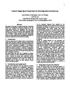
to reference the cell’s set of internal variable values [6]. Although the application of our generic automaton is not limited to cellular automata, this is a common use of these libraries. As a result, in our generic automaton we use the term “type” rather than ’state’ to avoid potential confusion. To interface with our generic automaton, the user must create some class to represent a simulation object, containing a variable representing the type of the object by a built-in type (i.e., unsigned char) - from now on we will use Object as the name of this class and type as the name of the variable. For a model with n different types we assume type to contain a value between 0 and n-1, with each value representing one type. Figure 1 expresses this design in UML. An abstract class Transition provides the interface for individual transitions. Transition contains a variable type which holds the destination type, and a function checkCondition() which returns ’true’ if the passed Object should switch to this type. checkCondition() accepts any necessary parameters to encompass all internal and external conditions relevant to the automaton, for example, a grid of chemical concentrations or the value of a global timer. A set of rules for changing type is contained within the class ObjectType. Each ObjectType contains an array of Transition objects, and by default the checkCondition() method of each added Transition is invoked in the ObjectType::update() function, potentially changing the type of the Object parameter. If all invocations to checkCondition() return false, the type of the Object does not change. The class Automaton supplies the highest-level interface, and each Automaton object may contain multiple ObjectTypes. We allowed this to give users more flexibility. For example, it may be desirable for an object to operate under different sets of rules depending on the current simulation status. The Automaton::update() function controls the set of rules to use and can be overridden accordingly in child classes. By default there is one ObjectType member, and its update() method is invoked in Automaton::update(). The State pattern defined by Gamma et al. accomplishes the same tasks but employs a slightly different design. They provide abstractness for states, we provide it for transitions. That is, their libraries define an abstract State class with a Handle() method, and each state in the automaton must define a class with parent State and a customized Handle() which can define object behavior and conditions for state changes. In our generic automaton, we provide an abstract Transition class, and a class must be defined for each type that has transitions coming in. Good extensibility is thus provided by both patterns – State makes it easy to add new types, our generic automaton makes it easy to add new transitions. State is likely better in terms of per-
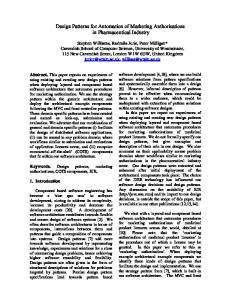
formance upon type transition - because since the current celltype is known, in the worst case n-1 transitions need to be checked versus n2 in the worst case for the generic automaton (although this will happen rarely since after one transition passes the checking stops). However, the generic automaton is easier to maintain. For an automaton with n types, in the State pattern n classes must be defined no matter what. In our generic automaton that number is ≤ n, because some types may only have transitions going out and not coming in. This actually happens in cellular automata used in many known morphogenesis models [12, 17]. Irreversible processes for example could also require these kinds of types. As more models are added that could potentially have lots of types, many of which do not transition anywhere, the overall size of the framework will grow much more rapidly with the State pattern. As an example application of the generic automaton, take the simple automaton shown in Figure 2. Assume there are three types A, B and C, and there is some static variable x defined. A is the initial type (pointed to by the caret). Note that A only has an arrow leaving it (none entering), therefore it is not necessary to define a transition class for A. Automaton
A x>3 x < 10
B
C x >= 10
Figure 2. Simple automaton with types A, B and C, dependent upon variable x.
Figure 1. Implementation of the generic automaton in UML. We can implement the automaton in a class SimpleAuto, and define transitions BTransition and CTransition: class BTransition :
public Transition {
class CTransition : public Transition { public: CTransition(char cellType) : Transition(cellType) {} bool checkCondition(Object* object) { return ((object->type == 1) && (x >= 10))); } }; class SimpleAuto : public Automaton { public: virtual void init(); unsigned char getObjectType(const Object *object) const; string getTypeName(const char type) const; unsigned char getTypeId(const string typeName) const; }; void SimpleAuto::init() { objectType = new ObjectType(); objectType->addTransition( new BTransition(1)); objectType->addTransition( new CTransition(2)); }
unsigned char SimpleAuto::getCellType(const Object* object) const { if (object->type == 0) return "A"; else if (object->type == 1) return "B"; else if (object->type == 2) return "C"; else error(1); } string SimpleAuto::getTypeName(const char type) const { switch (type) { case 0: return "A"; case 1: return "B"; case 2: return "C"; default: error(1); } } unsigned char SimpleAuto::getTypeId(const string typeName) const { if (typeName == "A") return 0; else if (typeName == "B") return 1; else if (typeName == "C") return 2; else error(1); }
The generic automaton libraries are available within the C OMPU C ELL framework on SourceForge [10]. Cell types in C OMPU C ELL are controlled by an Automaton object.
3.2. Plugins It can be desirable for scientific software to possess optional functionality, i.e. functionality that can be added or removed from a simulation without difficulty. For example, a biologist may want to observe cellular behavior with and without mitosis; a chemist may want to view the effects of adding or removing a chemical from a medium. Ideally to minimize executable size in memory, if functionality is excluded from a simulation, objects that implement this functionality should not be allocated. This can be accomplished by consolidating all functionality of one specific feature into a plugin object. A user can add or remove a plugin from a simulation through for example a configuration file or GUI using a specific plugin name. Through a plugin proxy, accomplishing the goals of the Proxy pattern of Gamma et al. [11] with a slightly different implementation, creation of the potentially large plugin object is performed on de-
mand. Standard Template Library maps from plugin names to plugin objects and corresponding factories [3] are kept by a plugin manager, and if a plugin is ‘included’ by the user, the appropriate factory in the factory map allocates the correct plugin object, and its functionality is accessed through the plugin map. Often in scientific software features can be interdependent. For example, a feature that implements cell growth may depend on another feature that controls chemical concentrations. Since this is the case, plugin interdependency is also desirable. For this reason, the plugin manager also contains a map from plugin names to BasicPluginInfo objects, which include the following data members along with appropriate accessors: • name (the name of this plugin) • description (a sentence describing the feature provided by this plugin) • numDeps (the number of other plugins that this plugin depends on) • dependencies (an array of the plugin names that this plugin depends on) The specific plugin is thus mapped to other plugins that it is dependent upon through the dependencies array, and upon creation of a plugin object, plugin objects for dependencies are also created. Before any plugin objects can be created, the factory and BasicPluginInfo maps of the plugin manager must be populated, so that upon inclusion of a plugin the correct factory can be invoked and the correct dependencies can be created. This process is called plugin registration. A BasicPluginProxy, from which all corresponding plugin proxies inherit, defines an init() method to accomplish this task. Upon registration from the proxy, the plugin manager stores the corresponding BasicPluginInfo object and the correct factory, but does not allocate a plugin object. Allocation as mentioned is performed at runtime for whichever plugins are included by the user. The UML inheritance structure for plugins is defined in Figure 3. A Proxy design pattern has been defined by Gamma et al [11]. Their proxy also accomplishes demand creation of potentially expensive objects, but their implementation is different. Their object proxy operates as a stand-in for objects, containing all methods of the object it is representing, but the object is only allocated if its data members are needed by an invoked method of the proxy. In our implementation, the proxy does not take the place of the plugin nor does it possess any of the plugin methods, but registers the plugin
Figure 3. UML diagram of the Plugin libraries. A new plugin is created by a factory object, following the factory design pattern [3]. All plugins are managed by a PluginManager. This object manages plugin attributes, objects, and factories. Plugins are registered with the manager through their respective plugin proxies.
it is representing in its constructor. The manager handles object allocation for included plugins. Here is the process for including an example plugin X, dependent upon plugins Y and Z: 1. XPluginProxy object is declared, and its constructor gets invoked. 2. XPluginProxy constructor registers a BasicClassFactory and a BasicPluginInfo object, including the name X and dependencies Y and Z, with the global plugin manager. 3. User specifies plugin X to be included, for example in a configuration file using the name X. 4. The manager is invoked and the factory array is accessed through the name X, finding the already registered BasicClassFactory object. 5. The create() method of the registered BasicClassFactory is invoked, creating an XPlugin object for the simulation.
6. The manager is invoked and the dependencies map is accessed through the name X, finding the already registered BasicPluginInfo object. 7. The dependencies data member of this object contains a list of plugin names upon which X depends, finding Y and Z. 8. Repeat steps 4-8 for Y and Z, including any of their dependencies. Plugins provide a clear structure for extension of a framework. As more features are added through plugins, the core functionality of the framework remains untouched, helping with maintenance. An additional feature implemented by plugins includes dynamic loading of plugin libraries through the use of an environment variable (for example PLUGIN PATH), which can be set for example in bash using: export PLUGIN PATH=/plugins
This provides more flexibility and makes the framework more customizable, enabling the user to have a single copy of the framework but several sets of plugins implementing different features, with the current ’active’ set of plugins determined by this environment variable. The loadLibraries() method of BasicPluginManager performs dynamic loading, accepting the library path as a string: BasicPluginManager pluginManager; pluginManager.loadLibraries (getenv(PLUGIN PATH));
C OMPU C ELL uses plugins to implement optional simulation functionality. Such options include: center of mass calculation, various CPM energy calculations, a densitydependent grid growth algorithm, polarity calculation, surface area calculation, and volume calculation. The user decides which functionality to include in an input configuration file. Cellular automata are implemented as plugins as well, which inherit the interface of Automaton. When an automaton is indicated in the configuration file, it is registered and subsequently run at every successful CPM flip. The generic plugin libraries are available in Coffland’s BasicUtils libraries [8], downloadable from SourceForge.
3.3. Dynamic Class Nodes In scientific simulations it is often necessary to keep track of several dynamic objects. In agent-based modeling [14] for example, there could be thousands to millions of agents with multiple attributes and properties, interacting with their surrounding environment(s) in various ways.
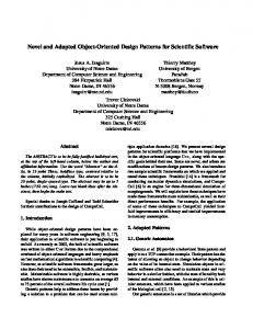
Molecular dynamics often imposes the need to record data for large quantities of atoms. There is a similar application to biological cell simulations and tracking individual cells. Large amounts of data cache misses and page faults can be generated by such applications. In particular, if individual object attributes are noncontiguously allocated in virtual memory and consistently needed throughout a simulation, a high swap rate could be imminent, potentially high enough to lead to thrashing as even recently used data needed in the near future gets swapped out. Contiguous attribute allocation for individual objects increases the likelihood of multiple attributes lying the same memory block, leading to the likelihood of lying in the same page, or even cache block. One way of providing contiguous allocation is through C structs, but these are lacking in terms of flexibility. In order to modify, add, or delete attributes, you must access a global struct, adding and deleting members accordingly. Dynamic class nodes provide more flexibility by allowing attribute registration in a similar way to plugins, while still enforcing contiguous allocation to avoid performance degradation due to thrashing and high cache miss rates. Each attribute is declared as a DynamicClassNode, and then registered through a BasicDynamicClassFactory. Each individual dynamic class node holds an offset, and so for example when a simulation object x is accessed, if an attribute y has offset z, the resulting address of attribute y is +z, for all simulation objects x. Figure 4 shows UML for an example dynamic class node for an attribute X, and Figure 5 shows the allocation of an object with three attributes that respectively consume 12, 8, and 12 bytes, using 4-byte memory blocks. BasicDynamicClassNodeBase + BasicDynamicClassFactory* factory + unsigned int offset + unsigned int getSize() + void _init(void*) + void* getNode(const void*) + void registerNode(BasicDynamicClassFactory*) + void setOffset(const unsigned int)
BasicDynamicClassFactory + unsigned int classSize + unsigned int numClasses + vector nodes + void* create() + void destroy(void*) + unsigned int getClassSize() + unsigned int getNumNodes() + unsigned int getNumClasses() + void registerNode(BasicDynamicClassNodeBase*)
Figure 5. Example allocation of a simulation object’s attributes represented as dynamic class nodes. Here is a code sample showing the addition of a dynamic class node representing center of mass (COM) to each simulation object, of size 12 bytes containing three integer coordinates x, y and z: class COM { public: int x; int y; int z; }
class COMDynamicClassNode : public BasicDynamicClassNode { virtual void init(COM *com) { com->x = com->y = com->z = 0; } }
The center of mass for a given object can now be accessed accordingly. For example to set an object’s x coordinate to 3: Object* myObject = (Object*) objectFactory.create(); comDCN.get(myObject)->x = 3;
X + type1 variable1 + type2 variable2 + type3 variable3
Figure 4. UML diagram of the dynamic class node interface.
C OMPU C ELL cell attributes (center of mass coordinates, volume, surface area, and type) are represented by dynamic class nodes. Many of these attributes are dynamic and play important roles particularly in Potts Model energy calculations. The dynamic class node libraries are also available in Coffland’s BasicUtils package [8].
3.4. Molecular Dynamics Patterns Molecular dynamics (MD) [4, 16, 22] is defined by particles (position and momenta) and their interactions (forces), the dynamics of the system are contained by integrating Newton’s equation of motion, i.e., the classical N −body problem. Solving the dynamics numerically and evaluating the interactions tends to be computationally expensive even for a few thousand particles. Specifically, the interactions are generally the computationally dominant part. For MD typical representatives of a scientific patterns are discrete problems that borrow techniques solving continuum problems to achieve better performance. The most relevant distinctions for these types of problems is between continuum and discrete systems, based on the description in [5]. Design pattern Conceptual model Description Classes
Design pattern Conceptual model Description Classes
Design pattern Conceptual model Description Classes Design pattern Conceptual model Description Classes
Design pattern Conceptual model Description Classes
Design pattern Conceptual model Description Classes
Particle-particle (PP) Discrete mechanics Point particle interactions defined by forces or potential Particle[position, velocity, mass, force, energy] Interaction[n-tuple potential and its relevant constants] Metric[defining distances and positions] SpatialManager[keeping track of spatial information] Modifier[function to modify the interactions] Selector[identifies the n-tuples] Integrator[intergration scheme] Particle-mesh (PM) Discrete and continuum mechanics Point particles are mapped to a grid; particles interact via the grid Particle[position, velocity, mass, force, energy] Grid[array of GridPoint’s] GridPoint[position, force and/or potential] Metric[defining distances and positions] Interaction[potential and its relevant constants] Modifier[function to modify the interactions] Interpolation[interpolation] Integrator[intergration scheme] Particle-particle-particle-mesh (P3 M) Discrete and continuum mechanics Combination of PP and PM; direct interaction and via the grid Combination of PP and PM Mesh (M) Continuum mechanics Continuous problem discretized on spatial grid Grid[array of GridPoint’s] GridPoint[position, force and/or potential] Interpolation[interpolation] Integrator[intergration scheme] Mesh-mesh (MM) Continuum mechanics Continuous problem discretized using a hierarchy of grids GridArray[array of Grid’s] Grid[array of GridPoint’s] GridPoint[position, force and/or potential] Interpolation[interpolation] Integrator[intergration scheme] Multi-grid (MG) Discrete mechanics Point particle interactions derived both from particle interaction and a hierarchy of grids Combination of P3 M and MM
Table 1. Dynamics simulation patterns.
The conceptual model of discrete systems have some object defining some general sets of objects and some relations among them. The relations define the dynamics of the system. Essentially all particle systems fall into this category, especially MD applications. The patterns of continuum systems can typically only be solved by an approximation to a set of points or grid of cells. The problem is reduced to a discrete form represented by some virtual set of objects and some relations among them. Typically representatives are fluid or field systems. Table 1 gives an overview of the 6 most relevant patterns for simulation of dynamics. This representation differs slightly from [5] and augments it with the Mesh-Mesh and Multi-Grid patterns. The multigrid pattern (MG) can be described by a combination of three basic patterns: PP: Fast varying short-range interactions, PM: Interaction between the particles and the finest grid, and MM: Interaction between the different grids. The multigrid pattern can be generalized as a way of creating a hierarchical model out of several different models that interact among each other. From our point of view it is more reasonable to treat the integration as a separate entity such that the force and integration definition are decoupled. This enables us to meet the requirements of arbitrary multiple stepping algorithms with arbitrary levels and arbitrary associated forces at each level, the approach of a chain of integrators was chosen (Figure 6). A chain of arbitrary length is defined by recursion, where a single time stepping (STS) integrator terminates the recursion, reflecting the idea of the Strategy Chain pattern. For the design of integrators, inheritance is appropriated, where MTSIntegrator doHalfKick(); doDriftOrNextIntegrator(); *nextIntegrator calculateForces(); doHalfKick();
Figure 6. Chain of integrators implementing multiple time stepping schemes. MTS differs from STS in that it calls recursively the next inner integrator before evaluating its forces. The recursion is terminated by an STS integrator.
MTS and STS integrators are two different main branches solving the dynamics. Inheritance is well-suited to capture the unique and shared behaviors of integrators. Furthermore, when defining an MD system with all its potentials and particles, and boundary conditions – the forces associated at each integrator level – one also must
compute the actual interactions between the particles, which can lead to a complexity of O(N 2 ) when using brute-force algorithms. In order to use different algorithms for different potentials and system requirements one needs to separate them to avoid code replication and enforce maintainability. Furthermore, the definition of potentials and numerical integration scheme cannot be hard coded, since they differ from application to application, and should ideally be created on demand. The idea of separation is captured by the Policy pattern, better known as the Strategy pattern [11, pp. 315-323]. This pattern promotes the idea to vary the behavior of a class independent of its context. It is well-suited to break up many behaviors with multiple conditions and it decreases the number of conditional statements. Closely related are Traits, which intend to carry some extra information of a class, but without requiring any changes of the class itself. Policies and Traits have a lot in common, but the Policies tend to be behavioral, whereas Traits allow subtyping. In P ROTO M OL the design of the forces is based on the Policy pattern and motivated by the Dynamics Simulation patterns from Table 1, where the following requirements are parameterizable: R1 An algorithm to select an n-tuple of particles to calculate the interaction. R2 Boundary conditions defining positions and measurement of distances in the system. R3 A component to retrieve efficiently the spatial information of each particle. This has O(1) complexity. R4 A potential defining the force and energy contributions on an n-tuple. R5 A component to modify the potential (force and energy contributions) to obtain certain properties of the potential, i.e., switching functions. The algorithm to select the n-tuples (R1) is customized with the rest of the four requirements (R2-R5). Some forces may not allow any parameterization at all since they are specialized and hand-crafted to carry out one particular case, e.g., propagating force contributions from an external device like a haptic device. At first, it seems more natural to customize the potential (R4) with an algorithm (R1), but after analyzing the general application requirements and their dependencies, it makes more sense in terms of design and efficiency to choose the first design approach. This becomes more obvious when we like to evaluate simultaneously different types of forces with the same algorithm. The overall design coupled of P ROTO M OL with the Factory, Singleton and Prototype patterns, and Policy pattern increases the maintainability of the framework, enabling us
to easily add new objects without changes across the framework. Furthermore, one can also customize the possible objects available to the user and exclude the objects that do not make sense.
4. Conclusions The application of these scientific patterns to C OMPU C ELL and P ROTO M OL validates their usability and potential benefits, and also reemphasizes the importance of design pattern research in software engineering. We hope that these scientific patterns will be helpful in future software releases, both by ourselves and researchers designing related software packages.
References [1] Software maintenance fox pro wiki. http://fox.wikis.com/wc.dll? Wiki˜SoftwareMaintenance˜SoftwareEng. [2] M. S. Alber, M. A. Kiskowski, J. A. Glazier, and Y. Jiang. On cellular automaton approaches to modeling biological cells. Technical Report 337, University of Notre Dame, Department of Mathematics, Sept. 2002. [3] A. Alexandrescu. Modern C++ design: generic programming and design patterns applied. Addison-Wesley, Reading, Massachusetts, 2001. [4] M. P. Allen and D. J. Tildesley. Computer Simulation of Liquids. Oxford University Press, New York, 1987. [5] C. Blilie. Patterns in scientific software; an introduction. Computing in Science and Engineering, 4(3):48–53, 2002. [6] R. Chaturvedi, J. A. Izaguirre, C. Huang, T. Cickovski, P. Virtue, G. Thomas, G. Forgacs, M. Alber, G. Hentschell, S. A. Newman, and J. A. Glazier. Multi-model simulations of chicken limb morphogenesis. In Computational Science—ICCS 2003, International Conference, Melbourne, Australia and St. Petersburg, Russia, pages 39–49. SpringerVerlag, Berlin, 2003. Lecture Notes Comput. Sci. 2659. Full paper review. [7] T. Cickovski, C. Huang, R. Chaturvedi, T. Glimm, H. Hentschel, M. Alber, J. A. Glazier, S. A. Newman, and J. A. Izaguirre. A framework for three-dimensional simulation of morphogenesis. IEEE/ACM Trans. Comp. Biol. and Bioinformatics, 2004. Submitted, preprint at http: //www.nd.edu/˜tcickovs/bare_jrnl.pdf. [8] J. Coffland. Basicutils. http://compucell. sourceforge.net/phpwiki/index.php/ BasicUtils, Dec. 2003. [9] COMPUCELL. http://www.nd.edu/˜lcls/ compucell, 2004. CompuCell home page. [10] COMPUCELL. C OMPU C ELL: A framework for threedimensional simulation of morphogenesis. http:// sourceforge.net/projects/compucell/, Aug. 2004. 253 downloads from Apr. 2003 - Aug. 2004. [11] E. Gamma, R. Helm, R. Johnson, and J. Vlissides. Design Patterns. Elements of Reusable Object-Oriented Software. Addison-Wesley, Reading, Massachusetts, 1995.
Design Pattern Generic Automation
Plugins
Dynamic Class Nodes
Policy MultiGrid Strategy Chain
Scientific Pattern Type/State Diagram
Optional Features
Simulation Object Attributes
MD potential definition and numerical integration scheme MD fast electrostatic evaluation Multiple time stepping integrator.
Description Invoked by simulation objects that must posses an internal state which determines their behavior, potentially dependent upon internal and external conditions. Implementation of a simulation feature that should be excluded or include, and this should be in the control of the user without modifying the source. Dynamic loaded. Implements contiguous allocation for attributes of each individual simulation object, with more flexibility provided by attribute registration. Varies the behavior of a class depending on its context. Linear-time algorithm for computing electrostatics. A chain of integrators implements a multiple time stepping integrator addressing the different time scales by splitting the forces
Sample Framework C OMPU C ELL
C OMPU C ELL
C OMPU C ELL
P ROTO M OL P ROTO M OL P ROTO M OL
Table 2. Summary of the scientific design patterns that we have used and the frameworks on which we tested them.
[12] F. Graner and J. A. Glazier. Simulation of biological cell sorting using a two-dimensional extended potts model. Phys. Rev. Lett., 69:2013–2016, 1992. [13] H. G. E. Hentschel, T. Glimm, J. A. Glazier, and S. A. Newman. Dynamical mechanisms for skeletal pattern formation in the vertebrate limb. Proc R Soc Lond B Biol Sci, 271(1549):1713–1722, 2004. [14] Y. Huang, X. Xiang, G. Madey, and S. Cabaniss. Agentbased scientific simulation using java/swarm, j2ee, rdbms and automatic management techniques. Preprint., 2004. [15] J. A. Izaguirre. Laboratory for Computational Life Sciences. http://www.nd.edu/˜lcls, July 2004. [16] A. R. Leach. Molecular Modelling: Principles and Applications. Addison-Wesley, Reading, Massachusetts, July 1996. [17] S. Maree. From Pattern Formation to Morphogenesis. PhD thesis, Utrecht University, Netherlands, Oct. 2000. [18] T. Matthey. Framework Design, Parallelization and Force Computation in Molecular Dynamics. PhD thesis, University of Bergen, Bergen, Norway, 2002. [19] T. Matthey and J. A. Izaguirre. ProtoMol: A molecular dynamics framework with incremental parallelization. In Proc. of the Tenth SIAM Conf. on Parallel Processing for Scientific Computing (PP01), Proceedings in Applied Mathematics, Philadelphia, Mar. 2001. Society for Industrial and Applied Mathematics. Full paper review. [20] C. Picioreanu, M. C. M. van Loosdrecht, and J. J. Heijnen. A new combined differential-discrete cellular automaton ap-
[21]
[22] [23] [24]
[25]
proach for biofilm modeling; application for growth in gel beads. Biotechnl. Bioeng., 57:718–731, 1998. PROTOMOL. P ROTO M OL: An object oriented framework for molecular dynamics. http://sourceforge. net/projects/protomol/, Aug. 2004. 554 downloads from Sept. 2003 - Aug. 2004. D. C. Rapaport. The Art of Molecular Dynamics Simulation. Cambridge University Press, 1995. T. Schlick. Molecular Modeling and Simulation - An Interdisciplinary Guide. Springer-Verlag, New York, NY, 2002. A. Shalloway and J. R. Trott. Design Patterns Explained: A New Perspective on Object-Oriented Design. AddisonWesley, Boston, MA, 2002. J. P. Tremblay and G. A. Cheston. Data Structures and Software Development in an Object-Oriented Domain. Prentice Hall, Upper Saddle River, NJ, 2001.