Detecting Network Communities: a new systematic and efficient ...

Detecting Network Communities: a new systematic and efficient algorithm Luca Donetti1 and Miguel A. Mu˜ noz1

arXiv:cond-mat/0404652v2 [cond-mat.stat-mech] 25 Oct 2004

1

Departamento de Electromagnetismo y F´ısica de la Materia and Instituto de F´ısica Te´ orica y Computacional Carlos I, Facultad de Ciencias, Univ. de Granada, 18071 Granada, Spain (Dated: February 2, 2008) An efficient and relatively fast algorithm for the detection of communities in complex networks is introduced. The method exploits spectral properties of the graph Laplacian matrix combined with hierarchical-clustering techniques, and includes a procedure to maximize the “modularity” of the output. Its performance is compared with that of other existing methods, as applied to different well-known instances of complex networks with a community-structure, both computer-generated and from the real-world. Our results are in all the tested cases, at least as good as the best ones obtained with any other methods, and faster in most of the cases than methods providing similarquality results. This converts the algorithm in a valuable computational tool for detecting and analyzing communities and modular structures in complex networks. PACS numbers: 89.75Hc,02.60Pn,05.50.+q

INTRODUCTION

The outburst of activity in the field of Complex Networks in recent years has been rather spectacular and amazing. Networks of any thinkable (and sometimes “unthinkable”) type, including social, biological and technological ones have been described, and their topological as well as dynamical features studied. A whole line of research has emerged and a new perspective to tackle complex problems created. See [1, 2, 3, 4, 5] for reviews from different perspectives and for exhaustive lists of references. One particular aspect, which has drawn much attention, is the existence of subsets of nodes highly linked among themselves but loosely connected to the rest of the network, i.e. communities. These are believed to play a central role in the functional properties of complex structures [6, 7]. Identifying communities and analyzing their nature is an important task in some fields as, for instance, computer science [8, 9], sociology [6, 10], biochemistry [11], bibliometrics [12], taxonomy, or, as a more specific instance, in the development of efficient search-engines for the WWW. According to Flake et al. [13], “as the web is self-organized into communities, search-engines implementing such a concept, would help surfers to find what they look for and avoid other contents”. The concept of “community” may be retained as rather vague and phenomenological. Indeed, depending on the network under scrutiny, it might be quite an artificial one, while, in other cases, it emerges as a very natural and useful structure-analysis tool. A way to make the concept more clear-cut and practical is through the definition of the modularity, Q (see below and [14, 15]), a quantity which provides a way to quantify the communitystructure of a given network. Other quantities have been proposed with the same purpose [7, 16, 17].

The problem of finding communities is not new and is closely related to the problem of graph-partitioning, profusely studied in the context of computer science [18, 19]. A review of some used techniques, including further references, can be found in [6, 20]. Related problems are image processing and pattern recognition, or more generically data-clustering: in these cases there is no underlying network, but instead some relation or similarity between existing elements can be estabilished [21, 22, 23]. In recent years many algorithms for detecting communities have been proposed, starting with the seminal work by Girvan and Newman [6, 14]. These authors proposed an iterative, divisive (as opposed to agglomerative) method based on the progressive removal of links with the largest betweenness, a quantity proportional to the number of shortest paths passing through a given edge [24]. The edges (or links) with the largest betweenness have the most prominent role in connecting different parts of the graph and, therefore, by removing them recursively a good separation of the network into its components or communities can be found. This method generates very good results and has been employed by different authors in studies of various kinds [25]. Unluckily, as already pointed out by the authors themselves, it has a main disadvantage: its computational demand is very high. For instance, for sparse networks with N nodes, the computation-time grows like N 3 . In order to deal with large networks, for which the previous algorithm turns out to be not viable, Newman himself developed a faster method (of the order N 2 ). It is based on the iterative agglomeration of small communities, starting from isolated nodes, by locally optimizing the modularity. This method generates worse results [26] than the previous one. Some alternative algorithms both divisive and agglomerative (which we do not attempt to exhaustively

2 overview here) have been proposed in the last months. Some of them are listed here in chronological order (see [20] for a more critical discussion of some of them): • The method by Radicchi-Castellano-CecconiLoreto-Parisi [17] is of order N 2 . It is a divisive algorithm that works nicely whenever triangular (or higher order) loops are present in the network. • Wu-Huberman algorithm [27]. It is a fast method (linear in N ), based on the idea of voltage drops, which visualizes the network as an electric circuit. It can be used to locate the community to which one specific node belongs, but it requires successive iterations of the method in order to provide a global network division in communities. • Reichardt-Bornholdt method [28]. In this recent paper the authors introduce an algorithm inspired in the celebrated super-paramagnetic clustering algorithm devised by Blatt, Wiseman and Domany [29]. It is based on a q-state Potts Hamiltonian, and allows, for the first time, for the identification of fuzzy communities. • Capocci-Servedio-Colaiori-Caldarelli method [30]. This algorithm combines the use of spectral properties (which are nicely reviewed and generalized to study different types of networks as, for instance, directed ones) with the use of correlation measurements to determine community closeness. • Fortunato-Latora-Marchiori method [31]. This is a variation of the method by Girvan and Newman, in which the betweenness is substituted by the alternative concept of information centrality, as a way to measure edge-centrality. The method generates good results but its performance (N 4 for a sparse graph) is rather poor. Apart from these techniques recently introduced in the field of complex networks, many other algorithms have been developed mainly in the context of computer science. Most of them employ spectral analysis, which provides, in a very natural way (using the first non-trivial eigenmode) a tool for bi-partitioning [32] as will be illustrated along this paper. By iterative applications of bi-partitioning more elaborated divisions into communities or components can be achieved [9, 33, 34]. Alternatively, some other spectral methods employ more than one eigenmode leading directly to a splitting [16, 35, 36]. Without neglecting any of these algorithms, which can be applicable depending on the situation under consideration, this paper introduces yet a new method, allowing for a systematic analysis and detection of communities. It combines the following features: i) the generation of good results in all the tested cases, ii) it is relatively fast, as compared with methods providing comparable results,

iii) it includes a way to optimize the output, as will be explained in what follows. The method proposed in this paper combines spectral methods with clustering techniques, and uses the concept of modularity in order to develop a working algorithm. More precisely, the main lines of the algorithm are as follows: spectral analysis of the Laplacian matrix allows us to project the network-nodes into an eigenvector-space of variable (tunable) dimensionality. Afterwards, a metric is introduced in various possible fashions, and then, finally, by applying standard clustering techniques a dendrogram [6] is built up. The modularity of possible groupings (sections of the dendrogram) is maximized for every considered dimension of the eigenvector-space and finally, the global maximum over all possible number of eigenvectors (i.e dimensions of the space) is found. In the forthcoming sections we review some basic ideas and definitions of spectral analysis and we introduce our algorithm step by step. Then we apply it to different workbench networks, comparing its performance with that of other existing methods and, finally, the conclusions are presented. USING THE LAPLACIAN EIGENVECTORS TO DETECT COMMUNITIES Spectral analysis: Laplacian eigenvectors

The topology of a network with N vertices can be expressed through a symmetric N ×N matrix L, the Laplacian matrix [37]. The diagonal elements Lii are given by the degree ki of the corresponding vertex i, while offdiagonal elements Lij are equal to −1 if an edge between the corresponding vertices i and j exists and 0 otherwise. The sum of elements over every fixed row or column is, trivially, equal to zero. Therefore, a “constant vector” (with all its components taking the same value) is an eigenvector with eigenvalue 0. Furthermore, since the quadratic form n X

Lij xi xj

i,j=1

can be written as

X

(xi − xj )2 ,

links

which is positive semidefinite, the eigenvalues of L are either zero or positive [38]. The use of other matrices, employed to study network spectral properties has been recently considered in [16, 30, 34]. If the graph under analysis is connected, there is only one zero eigenvalue corresponding to a constant eigenvector. On the contrary, for non-connected graphs (composed by m connected components) the Laplacian matrix

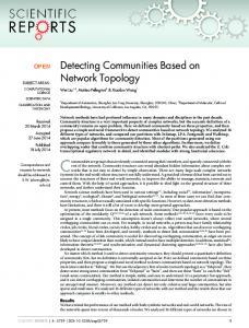
3 is block diagonal. Each block is the Laplacian of a subgraph and it admits a constant eigenvector with eigenvalue 0. Therefore, the Laplacian of the whole graph has m degenerate eigenvectors (corresponding to eigenvalue zero), each of them having nonzero constant components for nodes in the associated subgraph and 0 in the rest. If the subgraphs are not fully disconnected but, instead, a few links exist between them, the degeneration disappears. This leaves only one trivial eigenvector with eigenvalue 0 and m − 1 approximate linear combinations of the old ones with slightly non-vanishing eigenvalues [20, 30]. As the Laplacian matrix is real-symmetric, with orthogonal eigenvectors, and since the first of them has equal components, all the other ones must have components whose total sum vanishes. In order to illustrate how these ideas can be applied to identify communities, let us take, as a particular example, the number of subgraphs to be 2. In this case, the components of the second (first nontrivial) eigenvector are positive for one subgraph and have to be negative for the other, providing a clear-cut criterion to bisect the graph [32]. If the two subgraphs are not very well separated, then this distinction between positive and negative values becomes fuzzier. In such cases, more elaborated criteria to decide how to separate into two subgroups have been profusely studied in the specialized literature. Some of them optimize purposely defined quantities as the normalized cut [34] or the conductance [33], which are defined as functions of the number of links that exist between the two components and their sizes [39]. By iterating successive bisections, techniques to obtain more elaborate splittings can be constructed [9, 33, 34]. An alternative strategy is to assume that if there are more than two weakly-connected blocks it should be somehow possible to find them all by inspecting the eigenvalue spectrum more accurately, instead of considering just the first non-trivial eigenmode [35, 36]. Let us explore this idea, which is the one we will exploit, in more detail. Figure 1a shows the components of the first nontrivial eigenvector of a computer-generated graph including 4 communities, each composed by 32 nodes (see forthcoming sections for details). The group structure is clear, even if the two communities at the bottom are very near to each other and some nodes could be misclassified. In other examples, with a number of intergroup connections larger than here, the communities become more entangled, and the prospective of extracting clear-cut subdivisions using this type of one-dimensional plot worsens. This difficulty can be circumvented by taking into account some more eigenvectors, i.e. by enlarging the projection-space. This is illustrated in figure 1b, where the nodes of the same graph are plotted using the components on the first two nontrivial eigenvectors as coordinates. Simple eye-inspection shows that all communities are distinctly separated now. Actually, using three eigenvectors the nodes of the different groups fall

b

a 0.15

0.15

0.1

0.1

0.05

0.05

0

0

−0.05

−0.05

−0.1

−0.1

−0.1

−0.05

0

0.05

0.1

0.15

FIG. 1: (a) Components of the first non-trivial eigenvector for a computer-generated network with 4 communities (see main text). Two communities are clearly identified while the other two overlap. (b) All communities can be clearly identified when the components of the second eigenvector are plotted versus those of the first one; i.e. when the dimensionality of the eigenvector-space is enlarged.

around the vertices of a (slightly distorted) tetrahedron, with some further improvement in inter-community separation. Generalizing this idea, each vertex in the graph is represented by a point in a D-dimensional space in which the coordinates are given by its projections on the first D nontrivial eigenvectors.

Introducing a metric

Aimed at turning “eye-inspection” of communities into a more quantitative measure, the explicit introduction of a metric (or similarity measure) is required. The most straightforward choice would be the Euclidean distance. However, this is not the only possibility; another one is to consider the angular distance, defined as the angle between the vectors joining the origin of the D-dimensional space with the two points under consideration. This possibility is inspired by empirical observations: loosely connected nodes could be quite “Euclideanly” far from each other within a community, but still lying in the same “direction” in the eigenvector-space [41]. Moreover, when networks are large, nodes in the same community form a roughly one-dimensional “bundle” (see for example figure 3 in [8]). Note also, that using angular distances is tantamount to normalizing the position-vectors in the corresponding space and then measuring the Euclidean distance, similarly to what proposed in [36]. As will be shown, the angular metric generates, as a matter of fact, better results than the Euclidean one.

4 Cluster analysis

Having introduced a way to measure distances in the eigenvector space, a method to group nodes into communities is required. Such a method is provided by standard clustering techniques [18] as, for example, hierarchical clustering. Starting from N clusters, composed by individual nodes, the two closest ones are iteratively joined together. In order to define cluster-to-cluster distance or “closeness” (for a given metric) different criteria can be employed, generating among others, the following clustering algorithms [18]: • All possible pairs of nodes, taking one from each of the two clusters under examination, are considered. The minimum possible node-to-node distance is declared to be the cluster-to-cluster closeness. This leads to single-linkage clustering.

corresponding level. However, the clustering algorithm gives no hint about the “goodness” of such a partition. Modularity

In order to quantify the validity of possible subdivisions (obtained as explained above) and to optimize the chosen splitting, we use, following [14, 15], the concept of modularity. It is defined as follows: given a network division, let eii be the fraction of edges in the network between any two vertices in the subgroup i, and ai the total fraction of edges with one vertex in group i (where edges “internal” to each group have weight 1 while inter-group links are weighted 1/2). The modularity, Q, is then defined as X (eii − ai )2 . (1) Q= i

• Proceeding as before, but replacing the “minimum possible node-to-node distance” between pairs by the “maximum” one, complete-linkage clustering is defined. • Another possibility consists in taking the average distance between all possible pairs. This leads to group-average clustering. • A cluster is represented by a single point located at its “center of mass”; the cluster-to-cluster distance is defined as the node-to-node distance between these two points. This leads to centroid clustering. All these criteria have been broadly studied and applied. None of them can be proved to be generically more efficient than the others. In particular, the single-linkage method, being very simple, can be useful to analyze large data sets, and possesses some further mathematical advantages [18]. On the contrary, it has a tendency to cluster together, at a relatively low level, distant nodes linked successively by a series of intermediates. This is usually called chaining property, which constitutes in some cases a serious drawback. On the other hand, a convenient advantage of both, single and complete-linkage clusterings, is that only the ordering of the similarity measure is important: every other metric which produces the same ordering of distances leads to the same results. The output of these algorithms can be represented by a hierarchical tree usually called dendrogram. The starting single-node communities are the branch-tips of such a tree, which are repeatedly joined until the whole network has been reconstructed as a single component (see, for instance, figure 2 in [6]). Each level of the tree represents a possible splitting of the network into a set of communities, obtained by halting the clustering process at the

It measures the fraction of edges that fall between communities minus the expected value of same quantity in a random graph with the same community division. The maximization of modularity has been proposed as a possible way to detect communities; since a full maximization is not possible in practice (the algorithm would take an amount of time exponential in the number of nodes to explore all possible splittings) an approximate algorithm has been suggested [15]. In our case, modularity measurements are simply used to find the best splitting among all the possible partitions of the dendrogram obtained following the previous steps [14]. Other indeces quantifying the quality of splittings have been also proposed in the literature. Some of them are the “conductance”, the “performance”, and the “coverage” to name but a few (see [16] and references therein for more details). None of these taken by itself, provides a fully useful criterion; they have to be combined somehow. It seems that the modularity is a better, more efficient, choice. Implementing a functioning algorithm

Summarizing the ideas introduced in the previous subsections, our algorithm can be synthesized and implemented to build up a functioning algorithm as follows. First a few eigenvalues and eigenvectors of the network Laplacian matrix are computed. The question of what “a few” means will be tackled afterwards. Since the Laplacian is usually a sparse matrix and not all eigenpairs are required (that will require a time N 3 ) the relatively fast Lanczos method [42] can be employed. Nonetheless, the eigenvector computation is still the most computationally expensive step of the algorithm. For any given number D of eigenvectors (i.e. for a fixed dimension of the space) a similarity measure (or

5 1 0.9 0.8

Q max / Q real

0.7 0.6 0.5 0.4 0.3

angular distance, complete linkage euclidean distance, complete linkage angular distance, single linkage euclidean distance, single linkage

0.2 0.1 0

1

2

3

4

5

6

7

8

k out

FIG. 2: Maximum modularity found by the algorithm, divided by that of the known splitting of a computer generated random graph (see main text); the average over 200 graphs is plotted as a function of kout .

1

fraction of nodes correctly classified

metric) is chosen, providing a basis to apply one of the previously introduced clustering techniques. Typically, Euclidean or, better, angular distances are employed. Among the various hierarchical clustering methods available, we test single- and complete-linkage clustering algorithms. These two have the advantage that no new distances have to be calculated during cluster formation: when two subgroups merge to form a larger one, its distance to any other cluster is given by the shortest (singlelinkage) or by the largest (complete-linkage) of the distances from the two original components. As said before, single-linkage performs poorly in many cases owing to the previously discussed “chaining” property, converting complete-linkage in the preferential choice. Other linkage methods will be explored in the future; in particular, group-average linkage could be suitable when studying tree-like graphs [43]. An important difference between the way we apply clustering techniques and other standard applications is that we know in advance the underlying network structure. Using this knowledge we implement the constraint that two clusters are susceptible to be merged only if there exists a link between them in the original network. At every step of the clustering process the modularity is computed. Once the whole dendrogram is completed, the splitting with the maximum modularity is chosen as the output for the corresponding D. The optimal value of D to be taken is not known a priori, but since the eigenvalue calculation is the slowest part of the algorithm, we can repeat the hierarchical clustering using all possible values of D, and look up for the largest value of the modularity. Typically the largestmodularity vs. D curve exhibits a maximum whose corresponding splitting provides the algorithm final output. If, instead, the curve keeps on growing up to the largest D, the number of computed eigenpairs has to be enlarged, in order to extend the range of the curve, until a clear-cut maximum is pin-pointed.

0.9 0.8 0.7 0.6 0.5 0.4 0.3 0.2 0.1 0

1

angular distance, complete linkage euclidean distance, complete linkage angular distance, single linkage euclidean distance, single linkage 2

3

4

5

6

7

8

k out

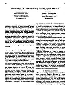
FIG. 3: Fraction of nodes of computer generated random graphs correctly identified by the algorithm, averaged over 200 graphs, as a function of kout .

TESTS OF THE METHOD Artificial community networks

To prove the algorithm we first test it on computergenerated random graphs with a well-known predetermined community structure [6]. Each graph has N = 128 nodes divided into 4 communities of 32 nodes each. Edges between two nodes are introduced with different probabilities depending on whether the two nodes belong to the same group or not: every node has kin links on average to its fellows in the same community, and kout links to the outer-world, keeping kin + kout = 16. In figures 2 and 3 we plot the modularity corresponding to the best splitting identified by the algorithm normalized by the one of the known answer, and the average

number of correctly classified vertices, respectively. Data for both, Euclidean and angular measures, and both, single- and complete-linkage algorithms, are shown. The number of eigenvalues leading to the largest modularity is between 3 and 5 for the angular distance, and between 2 and 4 for the Euclidean one. Let us remark that these are roughly equal to the number of communities and that the performance is much better using the angular distance. Summing up: on these computer-generated networks, our algorithm (equipped with the angular distance and complete-linkage) generates excellent results as compared with other methods (see, for instance, figure 1 in [15] and figure 3 in [31]).

6

0.319 0.368

TABLE I: Modularity of the best splitting of the Zachary club network obtained for different metrics and clustering algorithms.

0.5

0.5

0.4

0.4

0.3 0.2

modularity

0.412 0.412

modularity

single-linkage complete-linkage

single linkage clustering

complete linkage clustering

angular Euclidean

0.3 0.2

0.1

0.1

0

0

A1

A1

A2

A2

A3

A3

B1

B1

B2

B2

23 27

15

10

16

31 34

30

14

4

9

21

13

20

5 6

33

19

3 2

24

17

1

7

29

11

28 32

26 25

8

22

18

FIG. 5: Comparison between the final part of the dendrogram for the Zachary club, by using complete- and single-linkage clustering (bottom), together with the corresponding modularity values (top).

12

FIG. 4: Splitting of the Zachary club network. Squares and circles indicate the two communities observed by Zachary, colors denote the further subdivision found by our algorithm.

ently. Therefore, even if the best splitting is the same one in both cases, complete-linkage produces a more reliable dendrogram, describing more accurately the hierarchical structure.

Zachary karate club Scientific collaboration networks

Now we consider the well-known karate club friendship network studied by Zachary [44], which has become a commonly used workbench for community-finding algorithms testing [6, 14, 15, 17, 27, 28, 31]. Table I shows the maximum modularity found by the algorithm: the best value is again obtained using angular distances combined with either single or complete-linkage clustering. The best splitting is shown in figure 4; it is different from the “actual” breakdown of the club; i.e. the two groups reported by Zachary are further subdivided. Let us stress the presence of a single-node community (node 12), and the fact that the modularity value of this splitting is larger than Zachary’s one (0.371), and larger that the ones found using other methods [15, 28, 31]. In this case single and complete-linkage give the same best splitting. Nevertheless, the hierarchical structure given by the dendrogram in the two cases are quite different. Figure 5 shows how clusters merge after the best splitting is identified, as well as the modularity value corresponding to each division. For complete-linkage the modularity value remains close to the best one until the whole network is merged in one community. On the other hand, for single-linkage it falls down rather abruptly right after the first merging, owing to the chaining problem. Moreover, in the former case, the two Zachary communities are first reconstructed and then joined together, while in the latter the merging proceeds differ-

In order to test the method performance on larger networks we consider two scientific-collaboration networks first analyzed by Newman [45]. The vertices are the authors of the papers appeared in the cond-mat and hep-th archives at ArXiv.org between 1995 and 1999. Two authors are linked if they have co-authored a paper together. The cond-mat network contains 16726 nodes, but we focus on its largest connected component, which contains only 13861 authors. The computation of the first 1000 eigenvectors takes about two hours on a personal computer. The modularity curve computation, calculated using up to 999 eigenvectors, lasts around 15 minutes. Results for angular distance and complete-linkage clustering are plotted in figure 6. The largest value of the modularity, Q = 0.736, achieved for a splitting in 229 communities, corresponds to a 602-dimensional space. Obviously, we cannot compare the final splitting with a “true” one, which is not defined. As the curve in figure 6 is rather flat in its tail, one can legitimately wonder how does the best splitting compare to other ones obtained for similar dimensionalities. This question is difficult to answer in a rigorous way, and will deserve further analysis, which will eventually lead to a functional definition of the community-structure robustness. Analogously, the hep-th network has 8361 authors with a connected component of 5835. The largest mod-

7 cond-mat

the performance of the method.

modularity

0.75 0.7 0.65 0.6

0

200

400

D

600

800

1000

hep-th

modularity

0.75 0.7 0.65 0.6

0

200

400

D

600

800

1000

FIG. 6: Maximum modularity as a function of the number of eigenvectors for the cond-mat (top) and hep-th (bottom) networks.

ularity value, Q = 0.707, is produced by a division into 114 communities, obtained using 416 eigenvectors. The computation of the first 1000 eigenvectors takes around 30 minutes and the search of the largest modularity value about 8 minutes. In this case, the initial number of eigenvectors could have been taken much smaller than 1000, without affecting the final output, with the consequent time saving. As in previous cases, the number of eigenvectors used to produce the best splitting is of the order of magnitude of the number of found communities. In these cases, comparison with previous community studies is not feasible, as modularity measurements have not been (to the best of our knowledge) reported in literature.

CONCLUSIONS

We have introduced a new algorithm aimed at detecting community structure in complex networks in an efficient and systematic way. The method combines spectral techniques, cluster analysis, and the recently introduced concept of modularity. The nodes of the network are projected into a Ddimensional space, where D is a number of first nontrivial eigenvectors of the Laplacian matrix; their coordinates are the node-projections on each eigenvector. Then a metric (either Euclidean or angular) is introduced in such an eigenvector space. Once distances are computed, standard hierarchical clustering techniques (as, for instance, complete-linkage clustering) are employed to generate a dendrogram. The subdivision of this dendrogram giving the maximum modularity is taken as the output of the algorithm for a fixed D. Then, also D is allowed to vary (from 1 to some arbitrary, maximum value) providing a way to maximize the modularity and enhance

The best results are obtained using the angular distance and complete-linkage clustering; however, other types of distances, other clustering algorithms, or even other means to quantify the goodness of a division could be used to improve the results. In this sense our algorithm is a “block-modular” one: modifications of any of its ingredients could possibly lead to an overall improvement. Even if spectral methods have been profusely used before to analyze similar problems, we believe that our algorithm represents a step forward in studying complexnetwork communities, as it combines spectral techniques with (i) the novel concept of modularity, which provides a very adequate estimate of the quality of a given splitting and (ii) a way to optimize the number of eigenmodes taken into consideration. The weakest part of the method is that the maximum number of eigenvectors to be computed in order to find the one generating the maximum modularity is not known a priori. Being the calculation of eigenvectors the slowest part of the algorithm, what we do is to take a reasonable number of them and, afterwards, verify that the maximum-modularity curve as a function of D decreases at its tail; i.e. we make sure that a maximum of the modularity function is located. If this is not the case, the number of eigenvectors needs to be enlarged, at the cost of higher computational effort. In the absence of a general criterion to establish the monotonicity of the modularity curve, the only possible way to decide whether the identified local maximum is the global one, would be to compute all possible eigenvalues. In practice, in all the studied cases, the best splitting is found with a relatively small number of eigenvectors, converting the algorithm in a reliable, relatively fast, and very efficient one. An open challenge would be identifying a systematic criterion to estimate, a priori, what is the order of magnitude of the number of eigenvalues to be computed to further optimize the output and efficiency. We hope that this new algorithm will be employed with success in the search and study of communities in complex networks, and will help to uncover new interesting properties. We acknowledge useful comments and discussions with F. Colaiori, A. Capocci, V. Servedio, A. Arenas, G. Caldarelli, and J. Torres. We are specially grateful to M. Newman for providing us with the data on scientific collaborations as well as for a reading of the manuscript, and to C. Castellano, for very helpful comments and suggestions. Financial support from the Spanish MCyT (FEDER) under project BFM2001-2841 and the EU COSIN project IST2001-33555 is acknowledged.

8

[1] S. H. Strogatz, Nature 410, 268 (2001). [2] A. L. Barab´ asi, Rev. Mod. Phys. 74, 47 (2002). [3] S. N. Dorogovtsev and J. F. F. Mendes, Evolution of Networks: From Biological Nets to the Internet and WWW, Oxford University Press, Oxford (2003). [4] R. Pastor Satorras and A. Vespignani, Evolution and Structure of the Internet: A Statistical Physics approach, Cambridge University Press (2004). [5] M. E. J. Newman, SIAM Review 45, 167 (2003). [6] M. Girvan, M. E. J. Newman, Proc. Natl. Acad. Sci. USA 99, 7821-7826 (2002). [7] R. Guimer´ a, M. Sales-Pardo, and L. A. N. Amaral, cond-mat/0403660. [8] K. A. Eriksen, I. Simonsen, S. Maslov, and K. Sneppen, Phys. Rev. Lett. 90, 148701 (2003); and cond-mat/0312476. [9] C. Borgs, J. T. Chayes, M. Mahdian and A. Saberi, Proceedings of the 10th ACM SIGKDD International Conference on Knowledge, Discovery and Data Mining (2004). [10] R. Guimer´ a, L. Danon, A. Diaz-Guilera, F. Giralt, and A. Arenas, Phys. Rev. E 68, R065103 (2003); A. Arenas, L. Danon, A. Diaz-Guilera, P. M. Gleiser, and R. Guimer´ a, cond-mat/0312040. [11] L. H. Hartwell, J. J. Hopfield, S. Leibler, and A. W. Murray, Nature 402, C47 (1999). E. Ravasz, A. L. Somera, D. A. Mongru, Z. N. Olvai, and A. L. Barab´ asi, Science 297, 1551 (2002). [12] L. Egghe and R. Rousseau, Introduction to Informetrics, (1990). [13] G. W. Flake, S. Lawrence, C. L. Giles, and F. Coetzee, IEEE Computer 35, 66 (2002). [14] M. E. J. Newman, M. Girvan, Phys. Rev. E 69, 026113 (2004). [15] M. E. J. Newman, Phys. Rev. E 69, 066133 (2004) [16] U. Brandes, M. Gaertler, and D. Wagner. Proc. 11th Europ. Symp. Algorithms (ESA’03), LNCS 2832, pp. 568579. [17] F. Radicchi, C. Castellano, F. Cecconi, V. Loreto, and D. Parisi, Proc. Natl. Acad. Sci. USA 101, 2658-2663 (2004). [18] A. K. Jain and R. C. Dubes, Algorithms for clustering data, Prentice Hall, Englewood Cliffs, NJ (1988). B. S. Everitt, Cluster Analysis, Edward Arnold, London (1993). [19] E. Domany, Physica A 263, 158 (1999). [20] M. E. J. Newman, Eur. Phys. J. B 38, 321-330 (2004). [21] Y. Weiss, Proceedings IEEE International Conference on Computer Vision, 975-982 (1999). [22] R. O. Duda and P. E. Hart, Pattern Classification and Scene Analysis, Wiley. New York (1973). [23] K. Fukunaga, Introduction to statistical pattern recognition, Academic Press, San Diego (1990). [24] L. Freeman, Sociometry 40, 35 (1977). [25] J. R. Tyler, D. M. Wilkinson, and B. A. Huberman, in Proceedings of the First International Conference on Communities and Technologies, Ed. M. Huysman, E. Wenger, and V. Wulf, Kluwer, Dordrecht (2003). D. Wilkinson and B. A. Huberman, Proc. Natl. Acad. Sci. USA 101, 5241-5248 (2004). [26] The goodness of a given division (or division method) can be decided in absolute terms (when the underly-

[27] [28] [29] [30] [31] [32] [33] [34]

[35]

[36] [37] [38]

[39]

[40]

[41]

[42] [43] [44] [45]

ing community-structure is known, as for example, in computer-generated networks) or in relative terms (when the community structure is not known, but it maybe quantified in terms of modularity or similar measurements [14, 15, 17]; large modularity-values corresponding to better divisions). F. Wu, B. A. Huberman, Eur. Phys. J. B 38, 331-338 (2004). J. Reichardt, S. Bornholdt, cond-mat/0402349. M. Blatt, S. Wiseman, and E. Domany, Phys. Rev. Lett. 76, 3251 (1996); Neural Computation 9, 1805 (1997). A. Capocci, V. Servedio, F. Colaiori, and G. Caldarelli, cond-mat/0402499. S. Fortunato, V. Latora, M. Marchiori, cond-mat/0402522. M. Fiedler, Czech. Math. J. 23, 298-305 (1973) A. Pothen, H. Simon, K.-P. Liou, SIAM J. Matrix Anal. Appl. 11, 430-452, (1990) R. Kannan, S. Vempala, and A. Vetta, Journal of the ACM 51, 497-515 (2004) X. He, C. H. Q. Ding, H. Zha, and H. D. Simon, Proc. IEEE Int’l Conf. Data Mining, 195 (2001). C. H. Q. Ding, X. He and H. Zha. Proccedings 7th International Conf. on Knowledge Discovery and Data Mining (KDD 2001), 275 (2001). J. M. Kleinberg. Journal of the ACM 46, 604 (1999). D. Gibson, J. M. Kleinberg, and P. Raghavan. Proceedings of the 9th ACM Conference on Hypertext and Hypermedia, 225 (1998). A. Y. Ng, M. I. Jordan, and Y. Weiss, Advances in Neural Information Processing Systems 14, 849 (2002). N. L. Biggs, Algebraic Graph Theory, Cambridge University Press (1974). B. Mohar, The Laplacian spectrum of graphs, in: Y. Alavi, G. Chartrand, O. R. Ollermann, A.J. Schwenk (Eds.),Graph Theory, Combinatorics, and Applications, Wiley, New York, 1991, pp. 871-898. In principle the minimization of the conductance or the normalized-cut among all possible splits is a NP-hard problem. However, it can be shown that the cuts based on the components of the second eigenvector of the Laplacian or some related matrix give a guaranteed approximation to the optimal cut [36, 40]. F. Chung. Spectral Graph Theory, Number 92 in CBMS Region Conference Seriesin Mathematics. American Mathematical Society, 1997. The attentive reader could argue that figure 1b provides a counterexample to this general assertion; i.e. the two uppermost groups are nearby angularly but far apart Euclideanly. Indeed, taking the three-dimensional version of the net analyzed in such a figure, the four communities lay within the main directions on a tetrahedron, circumventing this apparent contradiction. G. H. Golub, C. F. Van Loan, Matrix Computations, Johns Hopkins University Press, Baltimore (1996). M. Newman, private communication. W. W. Zachary, J. of Anthropological Research 33, 452 (1977). M. E. J. Newman, The structure of scientific collaboration networks, Proc. Natl. Acad. Sci. USA 98, 404-409 (2001). See also, M. E. J. Newman, Phys. Rev. E 64, 016132 (2001).