Detecting Tangled Logic Structures in VLSI Netlists - SIGDA, Special ...

 

36.2

Detecting Tangled Logic Structures in VLSI Netlists Tanuj Jindal∗ , Charles J. Alpert‡ , Jiang Hu∗ , Zhuo Li‡ , Gi-Joon Nam‡ , Charles B. Winn‡‡ ∗ Department of ECE, Texas A&M University, College Station, Texas ‡ IBM Austin Research Lab, Austin, Texas ‡‡ IBM Systems and Technology Group, Essex Junction, Vermont

ABSTRACT

Most of the placement literature and all academic placers (e.g., [1] [2]) also assume that logic information is absent and operate purely at the gate level, instead of relying on hierarchical information. During this handoff between synthesis and placement, logic may be synthesized in such a way that it might require special care from the placement engine to obtain high quality results. Certain groups of logic will invariably have a higher degree of inter-connectivity than other groups. Let GTL denote a group of tangled logic. The automatic detection of GTLs has several potential applications:

This work proposes a new problem of identifying large and tangled logic structures in a synthesized netlist. Large groups of cells that are highly interconnected to each other can often create potential routing hotspots that require special placement constraints. They can also indicate problematic clumps of logic that either require resynthesis to reduce wiring demand or specialized datapath placement. At a glance, this formulation appears similar to conventional circuit clustering, but there are two important distinctions. First, we are interested in finding large groups of cells that represent entire logic structures like adders and decoders, as opposed to clusters with only a handful of cells. Second, we seek to pull out only the structures of interest, instead of assigning every cell to a cluster to reduce problem complexity. This work proposes new metrics for detecting structures based on Rent’s rule that, unlike traditional cluster metrics, are able to fairly differentiate between large and small groups of cells. Next, we demonstrate how these metrics can be applied to identify structures in a netlist. Finally, our experiments demonstrate the ability to predict and alleviate routing hotspots on a real industry design using our metrics and method.

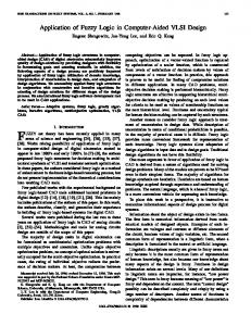
• Routability. Since a GTL has high interconnectivity, placement engine will naturally want to pull the cells tightly together which often will create a routing hotspot. Figure 1 shows a routing congestion map of a placed industrial design, in which the routing hotspots in the upper part of the design are caused by tangled logic structures that are placed too closely together. Later we show how simple process of cell inflation in a GTL can mitigate routing congestion. • Floorplanning. Since a GTL will stay together during placement, the designer may wish to form a soft block for the gates in the GTL. Then during placement, the soft block can be translated into placement constraints (like attractions, forces, or move bounds) to drive placement to a higher quality solution.

Categories and Subject Descriptors B.7.2 [Integrated Circuits]: Design Aids

• Logic re-synthesis. Synthesis will typically try to instantiate logic in the most compact form possible, yet this is one of the reasons why logic structures can be so tangled. Prior to placement, a GTL could be resynthesized or re-instantiated to utilize more area, but less interconnect, thereby reducing potential hotspots. Applying this technique to a small fraction of the design will not increase area dramatically.

General Terms Algorithms,Design

Keywords Rent Rule, Clustering, Tangled Logic, Congestion Prediction

1.

INTRODUCTION

The main problem this work addresses is how to find a GTL. Before one can find one, one should be able to somehow quantify how tangled a logic structure actually is. Therefore, we propose two new metrics derived from Rent’s rule to measure the quality of a GTL. The first metric allows one to explore the gamut of sizes between very small and very large cell groups and select the ones which best optimize the metric. Our second metric extends beyond Rent’s rule to account for internal connectivity. The reason a new metric is required is that existing cluster metrics cannot properly compare groups of cells of different sizes. When searching for GTLs one might find structures within structures, especially as the logic is repeated. We must be able to distinguish between them so that proper guidance can be given to the place-and-route tool. Our metrics and algorithm are able to decide whether we should choose several smaller GTLs or a much larger GTL which encompasses all the smaller ones. Our new metrics

During logic synthesis, high-level logic structures are translated into groups of logic gates. This synthesized netlist is then handed off to a place-and-route physical design flow. During this handoff, information about the origin of the logic that created the gates can be lost, especially if one switches from one tool vendor to another.  

Permission to make digital or hard copies of all or part of this work for personal or classroom use is granted without fee provided that copies are not made or distributed for profit or commercial advantage and that copies bear this notice and the full citation on the first page. To copy otherwise, to republish, to post on servers or to redistribute to lists, requires prior specific permission and/or a fee. DAC'10, June 13-18, 2010, Anaheim, California, USA Copyright 2010 ACM 978-1-4503-0002-5 /10/06...$10.00

 

603

36.2 Let the input netlist be represented as a hypergraph G = (V, E) where V is a set of cells and E is a set of nets, where each e ∈ E is connected to a subset of V . A clustering is a set of disjoint subsets of cells C1 ,C2 , ...,Ck ⊂ V such that V = C1 ∪C2 ∪ ... ∪Ck . Consider the literature of clustering metrics. 1. Given a cluster C, the net cut is defined as the size of the set / / Clustering metT (C) = |{e ∈ E|C ∩e 6= 0&(V −C)∩e 6= 0}|. rics can add the cuts in different ways, but fundamentally cut is independent of cluster size. It is more suited for top-down partitioning or placement, where the sizes of the regions are bounded. 2. Absorption [4] is a metric that counts the number of internal connections, and this will grow with clsuter size. It is illsuited for comparing two clusters as possible GTLs since the larger cluster will invariably have larger absorption. 3. The Ratio Cut and Scaled Cost metrics [5] both treat the cost (C) of a cluster as T|C| . Since T (C) grows much slower than cluster size, a larger cluster will almost always have smaller cost, which makes this a poor way to compare clusters of different sizes.

Figure 1: Example of routing hotspots.

are also scaled so that the average score of a typical cluster is one, and the ones with smaller values (e.g., less than 0.1) correspond to strong GTLs. This not only permits one to compare groups of different sizes, it also provides a uniform standard that can be utilized for different designs. Next we show how one can use the metric to actually find set of GTLs. Our algorithm starts from a random seed and grows a GTL by adding cells iteratively. We exploit parallalism to perform several such searches simultaneously and prune out the GTL candiates that are inferior and overlapping, resulting in an independent final set of identified GTLs. We validate our metrics and algorithm on random graphs, ISPD placement benchmarks, and a real industrial design. We demonstrate that our algorithm can identify GTL’s; and, application of cell inflation technique, within each GTL found, leads to reduced congestion in our industrial testcase.

2.

4. Ng et al. [6] proposed using the Rent exponent for a cluster as a way of measuring its quality, which means the cost of ln T (C) a cluster C is proportional to ln |C| . While this is better than ratio cut, it still monotonically decreases with size as C grows. 5. Hagen et al. [7] introduced the concept of DS(Degree Separation) metric. Degree is average number of nets incident on each node in the cluster and Separation is average length of shortest path between any two nodes. They make use of random walk to capture globally good circuit clustering. However, the metric fails to look at the external connection of cluster. Moreover, the authors used the average value of this metric to reflect the overall quality of clustering, not for a single cluster. 6. There are several relatively sophisticated metrics – (K,L)connectivity [8], edge separability [9] and adhesion [10], which are potentially useful for our case. However, these metrics require long computation time and also do not try to compensate for clusters of different sizes.

RELATED WORK

A GTL and a cluster are both a subset of netlist gates, so it might seem that one can apply traditional clustering metrics to GTLs. However, there are some clear differences between the problem statement of detecting tangled logic structures and cell clustering.

In summary, none of the clustering literature compares clusters of different sizes without biasing towards either smaller or bigger clusters. Our metrics are the first to do so.

1. Conventional clustering most often provides a reduction in problem size. These clusters are typically small (e.g., two to ten cells) so that too much information is not lost in the reduced problem instance. Clustering in this domain is generally local in nature [3]; however, this work is interested in identifying much larger special logic structures, of the order of hundreds to thousands of cells. This requires a more global view that accounts for both external and internal connections.

3. METRICS FOR TANGLED LOGIC STRUCTURES Our metrics are motivated by the need to (i) compare clusters of different sizes and (ii) measure the tangledness of the group of cells. We start with the ratio cut RC and Rent metric Rent for each cluster C, as discussed previously

2. Conventional clustering requires each cell to belong to a cluster, thereby covering the entire netlist. In contrast, we seek specific subsets of cells for special handling prior to placement. Thus, we wish to identify only a small fraction of cells as GTL’s and let place-and-route handle the other cells as it wishes.

RC(C) =

T (C) |C|

Rent(C) ∝

ln T (C) . ln |C|

The problem with both metrics is that the numerator (related to cut) and the denominator (related to cluster size) do not scale together. However, from Rent’s rule, we know that T (C) should grow

604

36.2 proportionally to |C| p , where p is the Rent exponent. Thus, we define the GTL-Score as GT L-S(C) =

internal connectivity versus external connectivity. Often in a design, MUX functions or logic look-up tables are synthesized to a group of complex cells, such as NAND4, OAI, and AOI gates since they generally give the most function per unit area. These gates generally have more pins (four or five) than most of the typical cells, such as AND2/OR2 gates (with three pins). All the connections required for these gates tend to tangle the logic and make the design harder to route. We need to capture the notion of pin-density without disturbing the essence of the normalized GTL metric. We propose to do so as follows:

T (C) |C| p

In general, one would expect this metric to be constant for an average quality structure. We do not care about tiny clusters with a handful of cells, nor partitions that consume a huge chunk of the circuit. Let A(G) be the total number of pins in G divided by |V |, i.e., A(G) is the average pin count of the cell. According to Rent’s rule, then A(G) is the expected value of GT L-S(C). Algorithmically, we want to have a rule of thumb about values of our metrics that identifies a good GTL, and this should be comparable across different netlists. Thus, we further refine our metric to the normalized GTL-Score nGT L-S(C) =

GT L-SD(C) =

T (C) AG · |C| p·AC /AG

where AC is the ratio of the number of pins contained in C divided by |C|, i.e., it is the average pin count of cells in the group. The ratio AC /AG is close to one when the number of pins inside C is typical relative to the rest of netlist. However, if C contains several complex gates, then this ratio will be higher than one and will reflect stronger likelihood of it being a GTL. Mutliplying this value by the Rent exponent biases the cost function to prefer groups of cells with higher pin count and consequently, more tangled logic. This will also provide a check for large cell groups and will identify them as GTL only if they have high density.

T (C) AG · |C| p

This will cancel out the differences between circuits with many high fanin versus low fanin gates. With this scaling, the score of an “average quality group” should be one. However, for a GTL, we would expect the value to be significantly smaller. To illustrate how the metric behaves in practice, consider a cell agglomeration procedure, which picks a random seed cell and then grows the group by iteratively adding highly connected neighbors. We illustrate the procedure through a generated random graph with 250000 cells, in which 40000 cells were made more highly connected internally and less connected externally than the rest of the graph, i.e., the graph had exactly one GTL of size 40000 cells.

Figure 3: Example of density-aware GTL-Score. Figure 3 shows the same curves as in Figure 2 but with our final GT L-SD score. Comparing the two figures shows that both metrics can reveal the known GTL with 40000 cells. However, the contrast of the local minimum of the GT L-SD score is more dramatic than the original metric.

Figure 2: Example of nGTL-Score. Figure 2 shows the nGTL-Score as a function of group size for two cell agglomerations. The first was in a set of cells outside the GTL. For this curve, the group starts at a value of 0.3 near group size 0 and then quickly rises and is asymptotically approaching 0.9. However, for the second group inside the GTL, the score rises all the way past 1.5 before dropping precipitously, reaching a local minimum of about 0.1 once the entire GTL was discovered. Adding more cells to the GTL that do not belong causes the score to rise further. The intuition behind this is that, as soon as we include all cells of a GTL in the group T (C) is much smaller that |C| p . And, once we start adding cells from outside the T (C) rises to asymptotically follow |C| p as proposed by Rent’s rule. So far, we have addressed the issue of comparing groups of different sizes, but the metric does not consider internal connectivity. For a logic structure to be tangled, it should have significantly more

4. A METHOD TO FIND GROUPS OF TANGLED-LOGIC Based on our new metrics, we propose a straightforward algorithm (tangled-logic finder) to identify GLTs. This method consists of three phases: • Phase I: linear ordering generation. • Phase II: initial candidate GTL generation. • Phase III: GTL refinement and pruning. Please note that Phase II and Phase III can be integrated with other linear ordering generation methods [11] as well.

605

36.2

4.1 Phase I: Linear Ordering Generation

didate Bˆ i with the best score of the proposed metrics is selected as the refined candidate corresponding to the initial candidate of Bi . This procedure is carried out for all initial candidates in B to obtain a set of refined candidates {Bˆ 1 , Bˆ 2 , ..., Bˆ m }. These refined candidates are compared with each other. If one has overlap with another and inferior GTL-Score, it is pruned out. The disjoint candidates remained at the end is the final set of GTLs discovered by our method. The point to be noted here is that all the three phases mentioned above can be computed for all m initial seeds in parallel with no interdependence. The only serial part of algorithm is the final comparison between m refined GTLs generated through parallel execution.

The linear order generation initializes the group with a seed cell, which is randomly generated. Then, it iteratively adds one cell at a time to the group. The candidates for the cell addition are the cells outside of the group, but with direct edge connections with the group. Among these candidates, we choose the one with the strongest connection with the group. We use a weighted number of nets to indicate the degree of connection. If a candidate cell vi has a net e connected to the group and this net has λ(e) pins outside of 1 the group, its weight is λ(e)+1 . Hence, a net has higher weight if it has greater portion of its pins inside the group. The connection 1 . We between vi and the group is defined by ∑e|vi ∈e,e∩C6=0/ λ(e)+1 use min-cut as a secondary criterion for breaking ties. In this context, we are simply trying to build groups of connected cells to generate a potential linear ordering. Since the cells are being added iteratively, the cost function is trying to maximize the connectivity. When selecting among the candidate cells, emphasizing the con1 nection ∑e|vi ∈e,e∩C6=0/ λ(e)+1 instead of min-cut alone is particularly important at the beginning of cell agglomeration. If a candidate cell is outside the GTL, it usually has weak connections with its neighbors. If we use min-cut as the primary criterion, it is quite likely that this cell is included into the growing group. Likewise, if a candidate cell is inside the GTL, it usually has strong connections with its neighbors and the min-cut criterion may easily exclude this cell. The order in which the cells are added determines the linear ordering. The preference of connection over net-cut leads to building denser groups with low external connectivity. Thereby, leading to addition of cells belonging to true GTL first to the growing group.

5. EXPERIMENTAL RESULTS The proposed metrics and methods are tested on various testcases: random graphs, ISPD placement benchmarks [12] and a realistic industrial circuit. The experiments are performed on a Linux server with 8 Intel Xeon processors of 3.2GHz frequency and 8G memory. The algorithm is implemented in C/C++ and parallelized using pthread in 8 parallel threads. In the experiments, the size of each linear ordering is at most 100K cells.

5.1 Experiments on Random Graphs The random graphs are generated based on [8] and its tangled logic structures are known a priori. The experimental results on the random graphs are shown in Table 1. The second column lists the number of nodes in each graph. The third column describes the synthesized GTLs in the graphs. For example, case 2 has two GTLs: one with 2000 nodes and the other with 15000 nodes. From the fifth column, one can see that our method can find all of the GTLs. In column 6, 7 and 8, the GTL sizes and the values of nGTL-Score (nGTL-S) and density-aware GTL-Score (GTL-SD) are reported. Column 9 tells the percentage of nodes which are in the known GTL but are missed by our method. Our method has zero missing nodes for 7 of the 10 GTLs. The maximum missing percentage is only 0.14%. Column 10 indicates the percentage of nodes which are not in the GTL but are included by our solution. This rate is also very low and no more than 0.5%. Since our method is to roughly point out the GTLs which need special treatment, missing a few cells or including a few more cells has negligible effect.

4.2 Phase II: Initial Candidate GTL Generation A cell group can be extracted from a linear ordering according to the metrics described in Section 3. A group C of size k = |C| is composed by the first k cells in the linear ordering. Then, the function nGT L-S(C) or GT L-SD(C) with respect to k is obtained like in Figure 2 and Figure 3. If there is a clear minimum in this function, the corresponding cell group is selected as a candidate GTL “B′′ . When computing the nGTL-Score, we need to decide the value of Rent exponent p. This is obtained by averaging the Rent exponents for all groups obtained in the linear ordering. The C Rent exponent of a group C can be estimated by ln T (C)−lnA where ln |C| AC is the average number of pins per cell in C. The procedure described so far is to identify a single GTL in the netlist. If the initial seed is outside of any existing GTLs, this procedure may fail like the flat curves in Figure 2 and Figure 3. To solve this problem, multiple searches starting with different seeds can be performed to generate a population of linear ordering and candidate GTLs B = {B1 , B2 , ..., Bm } for m parallel runs. If the number of searches is large enough, most of the GTLs can be captured.

5.2 Experiments on ISPD Benchmarks Since for ISPD placement benchmarks we have no knowledge about the existing GTLs in advance, we verify our metrics and method by correlating the solution generated with cell placement results. A placer normally places highly-connected cells close to each other, therefore the cells in a GTL found by our method are expected to be crowded in a small local region. Visualizations of cell placement and our tangled-logic finder solutions is illustrated in Figure 4. The clots with colors different from the majority of cells are the GTLs found by our method. Different color indicates different GTL. We further compared our metrics with ratio cut [5]. The curves of these metrics versus groups extracted from a linear ordering are shown in Figure 5. The top two curves correspond to the nGTLScore and the density-aware GTL-Score. The bottom curve is from T (C) ratio cut |C| . The ratio cut curve is much flatter and its global minimum is at its right end. This demonstrates that ratio cut overly favors large group size. Both of the top two curves have global minimum almost at the same place, i.e., they identify the same GTL. The one having the lowest minimum is from the density-

4.3 Phase III: GTL Refinement and Pruning A candidate GTL grown from a random seed might be slightly inaccurate. For instance, if the seed is at the boundary of an actual GTL, some cells outside that GTL might be included. In order to solve this problem, we enrich each initial candidate by additional candidate solutions. For each candidate Bi obtained in Phase II, we generate another set of candidates Bi,1 , Bi,2 , ..., Bi,l using seeds inside Bi and the same procedure as Phase I and II. These additional candidates are usually close to but slightly different from Bi . Then, union and intersection operations are performed on {Bi , Bi,1 , Bi,2 , ..., Bi,l } like in genetic algorithm. Finally, the can-

606

36.2 Table 1: Experimental results on random graphs. Case 1 2 3 4

Graph Information |V | Synthesized GTLs 10K 500 × 1 100K 2K × 1 + 15K × 1 100K 800K

5K × 1 40K × 6

#seeds 100 100

# GTL found 1 2

100 100

1 6

Tangled-Logic Finder Solutions GTL sizes nGTL-S GTL-SD Miss 501 0.1 0.085 0% 2010 0.025 0.022 0% 15003 0.017 0.0156 0.03% 5008 0.023 0.043 0% 40040 0.0095 0.001 0% 40092 0.0121 0.0209 0.04% 40053 0.0124 0.0214 0.14% 40044 0.0143 0.0015 0% 40044 0.0143 0.0015 0% 40006 0.0191 0.0021 0%

Over 0.2% 0.5% 0.05% 0.16% 0.1% 0.27% 0.28% 0.11% 0.11% 0.02%

Runtime(m) 1 33 31 141

estimated in 2-3 hours for a million nodes design by using both our method and our metrics. The current run-time obtained is in this range because we are issuing only 8 parallel threads at one time. But in industry, for practical application, we can afford to issue over 100 parallel runs in single step which can reduce the runtime dramatically by a factor of close to 2-5. Moreover, the quoted run-time still has a clear advantage on placement and routing that together takes close to 1 day.

5.3 Experiments on an Industrial Circuit The proposed metrics and methods are also tested on an industrial circuit. Figure 6 displays the tangled-logic finder solutions in cell placement. This is an industrial commercial ASIC design of 65nm technology. From the designers, we know that the blobs (shown as congestion hotspots in Figure 1) were originally ROM blocks, and were late dissolved to ordinary logic circuits to meet the timing closure. Therefore, these GTLs should have dense logic connections according to the designers. Figure 6 indicates that our method successfully finds these logic structures. In fact, the GTLs captured by our method in Figure 6 match almost exactly with the routing hotspots in upper part of Figure 1, which is from the same design. The characteristics of the solutions are summarized in Table 3. The first column lists the size of each GTL according to the circuit designers. The second column includes the size of the GTL found by our method. To show the usage of GTLs, all the cells inside the GTLs found through tangled-logic finder algorithm are inflated by four times, and placement was re-performed to spread these cells. Figure 7 shows the routing pictures for this new netlist. Note that since cells are inflated, so the new placement looks different than Figure 1 and Figure 6. It was observed that compared to original placement, the number of nets passing through 100% routing congested tiles are reduced from over 179K to 36K (5X reduction), and the number of nets passing through 90% congested tiles are reduced from 217K to 113K (2X reduction). The average congestion metric 1 is reduced from 136% to 91%. It is clear that better congestion can be achieved if placement employs cell inflation with GTLs identified with our technique.

Figure 4: GTL found by our method in Bigblue1. aware GTL-Score and the other one is from the nGTL-Score. The curve of nGTL-Score confirms our expectation that the value of nGTL-Score should be mostly around 1.

Table 3: GTLs found on the industrial circuit.

Figure 5: Functions of nGTL-Score (nGTL-S), density-aware (C) versus groups exGTL-Score (GTL-SD) and ratio cut T|C| tracted from a linear ordering of cells from Bigblue1.

Size of GTL in design 31880 31914 31754 32002 10932

The experimental results on the ISPD benchmarks are summarized in Table 2. It shows the circuit size |V |, number of seeds we used, number of GTLs founded and detailed information from 3 GTLs of each case. The rightmost column lists the total runtime of our 3-phase method in minutes. One can see that the GTLs can be

Size of GTL found 31835 31869 31803 32048 10952

Cut 36 36 36 36 28

GTL-Score 0.025 0.025 0.026 0.026 0.028

1 measured by taking the worst 20% congested nets and averaging the congestion number of all routing tiles these nets pass through

607

36.2 Table 2: Experimental results on ISPD 05/06 placement benchmarks. Case Bigblue1

|V | 278164

#seeds 100

# GTL found 72

Bigblue2

557786

100

93

Bigblue3

1096812

100

112

Adaptec1

211447

100

78

Adaptec2

255023

100

54

Adaptec3

451650

100

109

Top 3 GTLs Structure 1 Structure 2 Structure 3 Structure 1 Structure 2 Structure 3 Structure 1 Structure 2 Structure 3 Structure 1 Structure 2 Structure 3 Structure 1 Structure 2 Structure 3 Structure 1 Structure 2 Structure 3

GTL size 6187 1548 3539 13888 9602 10776 695 297 13005 2628 2616 375 751 3387 618 896 420 960

Cut 369 307 800 397 560 1091 81 76 2289 124 136 36 52 263 123 31 25 67

GTL-S 0.14 0.32 0.46 0.107 0.196 0.352 0.204 0.354 0.686 0.128 0.141 0.142 0.132 0.236 0.358 0.065 0.089 0.134

GTL-SD 0.031 0.083 0.14 0.045 0.111 0.195 0.225 0.202 0.454 0.083 0.093 0.212 0.315 0.058 0.435 0.058 0.17 0.126

Runtime(m) 81

104

159

77

114

142

6. CONCLUSIONS This paper introduces a new problem of finding tangled logic structures from synthesized netlists. These structures can help with floorplanning and routablility if special handling is given to cells in these structures. Our new metrics are the first ones to enable the comparison of clusters of different sizes and are normalized so that one can develop standards for tangled logic across a variety of netlists. We demonstrate a possible algorithm for discovering these structures and show how simply inflating the corresponding cells leads to much better routability after placement. Future work seeks to expand the metrics to handle more specialized structures driven by select lines, and to figure out new ways to use groups of tangled logic to drive better physical design solutions.

7. REFERENCES [1] T. Chen, T. Hsu, Z. Jiang, Y. Chang. NTUplace: a ratio partitioning based placement algorithm for large-scale mixed-size designs. In Proceedings of the International Symposium on Physical Degisn, pages 236–238, 2005. [2] T. Chan, J. Cong, J. Shinnerl, K. Sze, M. Xie. mPL6: enhanced multilevel mixed-size placement. In Proceedings of the 2006 International Symposium on Physical Design, pages 212–214, 2006. [3] C. J. Alpert, A. B. Kahng, G.-J. Nam, S. Reda, and P. Villarrubia. A semi-persistent clustering technique for VLSI circuit placement. In Proceedings of the ACM International Symposium on Physical Design, pages 200–207, 2005. [4] C. J. Alpert and A. B. Kahng. Recent directions in netlist partitioning: a survey. Integration: the VLSI Journal, 19(1-2):1–81, 1995. [5] P. K. Chan, M. D. F. Schlag, and J. Y. Zien. Spectral K-way ratio-cut partitioning and clustering. In Proceedings of the ACM/IEEE Design Automation Conference, pages 749–754, 1993. [6] T.-K. Ng, J. Oldfield, and V. Pitchumani. Improvements of a mincut partition algorithm. In Proceedings of the IEEE/ACM International Conference on Computer-Aided Design, pages 470–473, 1987. [7] Lars Hagen, Andrew B. Kahng A New Approach to Effective Circuit Clustering In Proceedings of the IEEE International Conference on Computer-Aided Design, pages 422–427, 1992. [8] J. Garbers, H. J. Promel, and A. Steger. Finding clusters in VLSI circuits. In Proceedings of the IEEE/ACM International Conference on Computer-Aided Design, pages 520–523, 1990. [9] J. Cong and S. K. Lim. Edge separability-based circuit clustering with application to multilevel circuit partitioning. IEEE Transactions on Computer-Aided Design, 23(3):346–357, March 2004. [10] P. Kudva, A. Sullivan, and W. Dougherty. Metrics for structural logic synthesis. In Proceedings of the IEEE/ACM International Conference on Computer-Aided Design, pages 551–556, 2002. [11] C. J. Alpert and A. B. Kahng. A general framework for vertex orderings with applications to circuit clustering. IEEE Transactions on VLSI Systems, 4(2):240–246, June 1996. [12] G.-J. Nam, C. J. Alpert, and P. G. Villarrubia. ISPD 2005/2006 Placement Benchmarks, pages 3–12. Springer, 2007.

Figure 6: GTL of the industrial circuit.

Figure 7: Routing congestion after cell inflation using GTLs information.

608