SS was partially supported by the William. R. and Sara Hart Kimball Stanford Graduate Fellowship. AMS 2000 subject classifications: .... Throughout Bin(n, p) will stand for a generic binomial random variable with n â N trials and success ...
DETECTION THRESHOLDS FOR THE β-MODEL ON SPARSE GRAPHS∗ By Rajarshi Mukherjee† , Sumit Mukherjee‡ , and Subhabrata Sen†
arXiv:1608.01801v1 [math.ST] 5 Aug 2016
Stanford University† and Columbia University
‡
In this paper we study sharp thresholds for detecting sparse signals in β-models for potentially sparse random graphs. The results demonstrate interesting interplay between graph sparsity, signal sparsity, and signal strength. In regimes of moderately dense signals, irrespective of graph sparsity, the detection thresholds mirror corresponding results in independent Gaussian sequence problems. For sparser signals, extreme graph sparsity implies that all tests are asymptotically powerless, irrespective of the signal strength. On the other hand, sharp detection thresholds are obtained, up to matching constants, on denser graphs. The phase transition mentioned above are sharp. As a crucial ingredient, we study a version of the Higher Criticism Test which is provably sharp up to optimal constants in the regime of sparse signals. The theoretical results are further verified by numerical simulations.
1. Introduction. Real life networks are ubiquitous in the natural and social sciences. Over the last decade, a huge volume of data has been collected on the structure of large networks and dynamics on these systems. Specialists from a wide array of disciplines such as physics, biology, social science, computer science, and statistics have studied these complex systems using specialized techniques. This area has seen an explosion of research in the recent years, and the resulting confluence of diverse ideas has enriched this field of study. From a statistical perspective, one avenue of research has focused on designing random graph models which exhibit some properties of real world networks such as a heavy-tailed degree distribution (Barab´ asi and Albert, 1999), a “small world” characteristic (Watts and Strogatz, 1998), etc. There has also been some preliminary work on testing for goodness of fit of these models to real data (Bickel et al., 2011). A parallel line of research has focused on the design and analysis of algorithms for finding structural patterns or ‘motifs’ in network data. Finding these structures is of interest to practitioners in diverse research areas as they often represent functional relationships between the vertices. For example, in a social network setup, a group of vertices with a high edge density may represent a community of individuals who share some common characteristics, e.g. a common profession. Guarantees for relevant statistical algorithms are usually derived by analyzing their typical performance on specific random graphs. Prominent examples include finding a single planted community or finding two equal sized communities in a graph. The simpler problem of detecting the presence of these structural patterns is itself statistically challenging, as they are often rare, and thus one needs to design procedures which work in a low signal to noise ratio setup. This has been accomplished for the single community case in (Arias-Castro and Verzelen, 2013; Verzelen and Arias-Castro, 2015). This body of work connects to the broader statistical program of global testing against structured alternatives (Ingster and Suslina (2003), Donoho and Jin (2004), Arias-Castro, Donoho and Huo (2005), Arias-Castro et al. (2008), Addario-Berry et al. (2010), Hall and Jin (2010), ∗
RM is a Stein Fellow at Department of Statistics, Stanford University. SS was partially supported by the William R. and Sara Hart Kimball Stanford Graduate Fellowship. AMS 2000 subject classifications: Primary 62G10, 62G20, 62C20 Keywords and phrases: Detection Boundary, Sparse Random Graphs, Beta Model, Sparse Signals
1
2
Ingster, Tsybakov and Verzelen (2010), Arias-Castro, Cand`es and Plan (2011), Cai and Yuan (2014), Arias-Castro and Wang (2015), Mukherjee, Pillai and Lin (2015)). It is well-known in social science that vertices of a network are often differentially “attractive”, with the more popular vertices having a higher tendency to form edges. Finding the vertices with higher “attractiveness” is of interest in a number of different contexts— they often represent highly influential nodes and practitioners might wish to screen these vertices for subsequent study. In an online social network, these vertices might actually represent spam accounts which should be detected and removed. In this paper, we formulate and address the question of detecting differential attractiveness of vertices in networks. While this question is statistically simpler, we expect that mathematically probing the limits of detection can also provide non-trivial information about the corresponding estimation question. The detection problem is of independent interest in a different context— assume that given a network dataset, one wishes to fit a stochastic block model to capture the community structure present in the data. It is well known that differential attractiveness of vertices can confound and affect model fits in this case (Karrer and Newman, 2011; Yan et al., 2014). Detecting the presence of this structural pattern is therefore imperative in this scenario. We believe that similar testing questions could be useful even in such setups. 1.1. Framework. Formally, we observe a labeled graph G = (V, E). We define |V | = n and we are mainly interested in the asymptotic regime where the graph size n → ∞. The graph G can be equivalently described by the adjacency matrix Y = (Yij : 1 ≤ i, j ≤ n), where Yij = 1 if {i, j} ∈ E and Yij = 0 otherwise. We note that trivially, Yij = Yji while Yii = 0, as we consider graphs without loops. Next, we specify a statistical model for the graphs in this context. For any β: = (β1 , · · · , βn ) ∈ Rn and λ ∈ [1, n], we define a probability distribution on the space of labelled graphs by setting (1.1)
Pβ,λ (Y) =
Y
1≤i 0 we let HC(t): =
n X i=1
Di = q
(I (Di > t) − Pβ=0,λ (Di > t)) ,
di −
λ 2n (n
− 1)
λ 1− (n − 1) 2n
λ 2n
�,
i = 1, . . . , n.
We then construct a version of the higher criticism test as follows. Define ( ) p HC(t) HC: = sup GHC(t): = p , t ∈ { 2r log n: r ∈ (0, 5)} ∩ N . V arβ=0,λ (HC(t))
By Higher Criticism Test we then mean a testing procedure that rejects when the observed value of HC defined above is large (See proof of Theorem 3.2 ii. a)). Indeed this test is designed along the tradition of tests introduced and studied in recent history of sparse signal detection in sequence and regression models (Donoho and Jin (2004); Hall and Jin (2010); Arias-Castro, Cand`es and Plan (2011); Arias-Castro and Wang (2015); Mukherjee, Pillai and Lin (2015); Barnett, Mukherjee and Lin (2016)). However, in spite of the similarity in philosophy of construction of the test, sharp analysis of the test turns out to be subtle due to the presence of dependence among the degree sequence. Interestingly, the case of relatively sparser graphs, with λ behaving polylogarithmically in n turns out to be easier. Since our results are valid for any λ ≫ log n, more care is needed to attend to the dependence structure in the problem. Tackling these dependence issues is fundamentally different from analyzing a weakly dependent Gaussian sequence (Arias-Castro, Cand`es and Plan, 2011). 3. Main Results. We divide the main results according to signal sparsity α ∈ (0, 1). Our first theorem corresponds to the dense regime of signal sparsity i.e. α ≤ 12 .
5
SHARP THRESHOLDS FOR β MODEL
Theorem 3.1.
Suppose α ≤
1 2
and let Cdense (α) =
1 − α. 2
i. The Total Degree Test is asymptotically powerful if n−r tanh(A) ≥ √ , λ
r < Cdense (α).
(3.1)
r > Cdense (α).
(3.2)
ii. All tests are asymptotically powerless if n−r tanh(A) ≤ √ , λ
We note that one can actually state a slightlyq stronger result which dictates that all tests are asymptotically powerless when limn→∞ s tanh(A) nλ = 0 while the Total Degree test is asymptotq ically powerful whenever there exists a diverging sequence tn → ∞ such that s tanh(A) nλ ≫ tn .
Our next result characterizes the detection thresholds in the sparser regime i.e. α > 21 . Unlike the denser regime (α ≤ 21 ), the results here depend on the level of graph sparsity λ. In particular for small λ’s (very sparse graphs) all tests turn out to be asymptotically powerless irrespective of the signal strength. Theorem 3.2.
λ , and let Suppose α ∈ (1/2, 1), θ: = limn→∞ 2n ( � 1 16(1 − θ) α − 12 , 2 Csparse (α). λ b) All tests are asymptotically powerless if r C ∗ log n , tanh(A) ≤ λ
C ∗ < Csparse (α).
Some remarks are in order regarding the results presented in Theorem 3.2. Indeed the detection limits presented above is reminiscent of those in Mukherjee, Pillai and Lin (2015). However, where results in Mukherjee, Pillai and Lin (2015) in essence correspond to λ = n, Theorem 3.2 presents a richer class of phase transitions by taking into account a continuous family of parameters θ: = lim λ/2n. However, the proof of such a result is simpler than that presented here due to the lack of dependence structure in traditionally studied regression models. Of course, the essence of our proof rests on understanding and carefully isolating the dependence structure present, and thereby reducing the calculations to a simpler independent binomial sequence problem. The subtlety of the proof relies on keeping track of the errors accumulated in such reductions. Finally, although
6
the proof of the lower bound (Theorem 3.2ii.b)) follows a general scheme of bounding a truncated second moment, deciding on the truncation event is subtle. Theorem 3.2 establishes the sharp optimality of the Higher Criticism Test in the sparse signal regime. Another commonly studied test of practical interest is the Maximum Degree Test introduced in Section 2. Our next theorem characterizes the detection limits of the Maximum Degree Test. Theorem 3.3.
Suppose α ∈ (1/2, 1), θ: = limn→∞
λ 2n ,
Cmax (α) = 16(1 − θ) 1 −
and let
√ �2 1−α .
i. Assume λ ≫ log n. Then the Maximum Degree Test is asymptotically powerful if r C ∗ log n tanh(A) ≥ , C ∗ > Cmax (α). λ ii. Assume λ ≫ log3 n. Then the Maximum Degree Test is asymptotically powerless if r C ∗ log n , C ∗ < Cmax (α). tanh(A) ≤ λ The results in Theorem 3.3 establish that for λ ≫ log3 n, the Maximum Degree Test is sharp optimal iff α > 3/4, and looses out to the Higher Criticism Test in the regime of α ∈ (1/2, 3/4). Although this result is parallel to those observed in sparse detection problems for independent Gaussian and Binomial sequence models (Arias-Castro, Cand`es and Plan, 2011; Mukherjee, Pillai and Lin, 2015), the proof of this fact is substantially more involved. This is in particular true about the proof of the lower bound part in Theorem 3.3ii.. Also note that Theorem 3.3i. hold as soon as λ ≫ log n. However, in order to prove the lower bound part in theorem above we crucially make use of the null distribution of maxni=1 di , which is readily available for λ ≫ log3 n (Bollob´as, 2001). The situation becomes highly subtle for log n ≪ λ . log3 n. In particular, we were able to argue that for log n √ ≪ λ . log3 n, if one considers the Maximum Degree Test that rejects when n maxi=1 di > npn + δn npn qn log n, where pn = λ/2n, qn = 1 − pn , and δn is some sequence of real numbers, then such tests are asymptotically powerless as soon as C ∗ < Cmax (α) defined above, if lim sup δn 6= 2. Lowering the requirement of λ ≫ log3 n to λ ≫ log n in this case requires a second moment argument along with Paley-Zygmund Inequality. We refer to Appendix D for more details. On the other hand, the case when lim sup δn = 2 is extremely challenging, and the result of the testing problem depends on the rate of convergence of δn to 2 along subsequences. We leave this effort to future ventures. 4. Simulation Results. We now present the results of some numerical experiments in order to demonstrate the behavior of the various tests in finite samples. To put ourselves in context of our asymptotic analysis, we chose to work with n = 100. Since our theoretical results depend both on the signal sparsity and graph sparsity, we divide our simulation results accordingly. In each of the situations, we compare the power of the tests (Total Degree, Maximum degree, and Higher Criticism respectively) by fixing the levels at 5%. In particular, we generate the test statistics 100 times under the null and take the 95%-quantile as the cut-off value for rejection. The power against different alternatives are then obtained empirically from 100 repeats each. Our first set of simulations corresponds to the dense regime i.e. α ≤ 12 . In figure 1, we plot the power of each of the three tests for a range of signal sparsity-strength pairs (α, r), where α ∈ (0, 21 ) −r with increments of size 0.025 and the signal strength is given by A = n√λ with r ∈ (0, 21 ) with
7
SHARP THRESHOLDS FOR β MODEL
0.4
0.4
0.4
0.3
0.3
0.3
0.2
0.2
0.2
0.1
0.1
0.1
0.0
0.0 0.0
0.1
0.2
0.3
0.4
0.5
0.5
0.0
0.0 0.0
0.1
0.2
α
(a)
1.0
r
0.5
r
0.5
r
0.5
0.3
0.4
0.5
0.0
0.1
0.2
α
(b)
0.3
0.4
0.5
α
(c)
Fig 1. The power of testing procedures in the dense signal setup. (a) shows the power of the Total degree test, (b) plots the max-degree while (c) plots the power of the GHC statistic . The theoretical detection threshold is drawn in red.
increments of size 0.025, and λ = 25. In addition, we plot the theoretical detection boundary given by r = 12 − α in red. As dictated by our theoretical results, the phase transitions are clear in the simulations as well. In particular, we observe that the Total Degree Test performs better in the dense regime. The Higher Criticism Test seems to have some power, the Maximum Degree Test fails have any power in this regime of sparsity. Our second set of simulations corresponds to the sparse regime i.e. α > 12 . In this case, following the theoretical predictions, we divide our simulations based on the graph sparsity λ as well. In figure 2, we plot the power of each of the three tests for a range of signal sparsity-strength pairs (α, r) for three different values of λ, namely λ = 2, 10, or 25 respectively. Specifically we choose for signal sparsity index varying between α ∈ ( 12 , 1) with increments of size 0.025, the signal strength q n to be A = C log with C ∈ (0, 16) with increments of size 0.5. In addition, we plot the theoretical λ √ detection boundary given by r = Csparse (α): = 16(1 − θ){(α − 1/2)I(α < 3/4) + (1 − 1 − α)2 I(α ≥ 3/4)} with θ = λ/2n, in red. To distinguish between the performance of the Higher Criticism Test and the Maximum Degree Test, we also plot the theoretical detection boundary of the Maximum Degree Test in cyan. The simulation results seem to match the theoretical predictions. In particular, when is λ < log n = 3, none of the tests seems to have any power in detecting any signal presented. In contrast for λ much larger than log n, the empirical performance of the Higher Criticism Test and Maximum degree Test also follows the theoretical guarantees. 5. Discussion. In this paper we formulate and study the problem of detecting the presence of differentially attractive nodes in networks through a version of the β-model on sparse graphs. Our mathematical results are sharp in all regimes of signal strength as well as graph and signal sparsity. The model can be further generalized, where instead of using an expit function, the connection probabilities between node i and j is given by nλ ψ(βi + βj ) for some function ψ which is the distribution function of a symmetric random variable, i.e. ψ(x) + ψ(−x) = 1, and satisfies some reasonable smoothness type regularity conditions. This in particular, will include the probit link Rx −t2 /2 √ e / 2πdt. Thereafter, similar to Mukherjee, Pillai and Lin (2015), we believe that ψ(x) = −∞
one can obtain parallel results here as well, with the sharp constants in the problem changing according to the function ψ. All of our results assume the knowledge of the graph sparsity parameter λ. In practice, this can
8
GHC
Max Degree
Total Degree
10
10
10
C
15
C
15
C
15
λ= 25 5
5
0
5
0 0.5
0.6
0.7
α
0.8
0.9
1.0
0 0.5
0.6
0.7
α
0.8
0.9
1.0
10
10
10
0.6
0.7
0.5
0.6
0.7
0.5
0.6
0.7
α
0.8
0.9
1.0
0.8
0.9
1.0
0.8
0.9
1.0
C
15
C
15
C
15
0.5
λ= 10 5
5
0
5
0 0.5
0.6
0.7
α
0.8
0.9
1.0
0 0.5
0.6
0.7
α
0.8
0.9
1.0
10
10
10
C
15
C
15
C
15
α
λ= 2 5
5
5
0
0
0
0.5
0.6
0.7
α
0.8
0.9
1.0
0.5
0.6
0.0
0.7
0.5
α
0.8
0.9
1.0
α
1.0
Fig 2. The power of the testing procedures in the sparse signal setup. The theoretical detection thresholds are drawn in red, while the thresholds for the Maximum Degree Test are drawn in cyan.
9
SHARP THRESHOLDS FOR β MODEL
be overcome by choosing a vertex at random and estimating λ by the proportion of its neighbors. Since s ≪ n, a randomly chosen vertex belongs with high probability to the set of vertices with √ corresponding βi = 0, and as a result it is not too hard to show that the resulting estimate is nconsistent in ratio scale. One can then delete this randomly chosen vertex from the network and consider the detection problem on the remaining n − 1 vertices. It indeed remains a question about how the performance of the corresponding testing procedures change according to this procedure. Although the analysis of the Total Degree Test and the Maximum Degree Test should not be too difficult to carry out following similar techniques to those carried out here, the analysis of the Higher Criticism Test is extremely subtle and is beyond the scope of the current paper. Although we only study the sparse detection problem in this paper, the rich phase transitions observed hint at similar complexities in further inferential questions. Of particular interest is the subset selection problem, which corresponds to the identification of vertices of differential attractiveness. We plan to address sharp analyses of such inferential questions in future papers. 6. Proofs of main results. In this section, we prove the main results in this paper. 6.1. Some properties of Binomial distribution. In this section, we collect some properties of the binomial distribution which will be used throughout this paper. The first lemma is a simple change of measure argument and the proof is omitted. Lemma 6.1.
If X ∼ Bin(n, p) then for any a > 0 and Borel subset of B of R � � � � � ap ∈B . E aX 1X∈B = (ap + (1 − p))n P Bin n, ap + (1 − p)
The next lemma is crucial and the proof is deferred to Appendix A.
Lemma 6.2. (a) Suppose Xn ∼ Bin(n, pn ) such that n min(pn , 1 − pn ) ≫ log n, and {Cn }n≥1 is a sequence of reals converging to C > 0. Then we have (i) � � p C2 1 P Xn = npn + Cn npn (1 − pn ) log n = √ n− 2 +o(1) , npn and
(ii)
� � p C2 lim P Xn ≥ npn + Cn npn (1 − pn ) log n = n− 2 +o(1) .
n→∞
(b) Suppose further that Yn ∼ Bin(bn , p′n ) is independent of Xn , and lim sup pn < 1, n→∞
bn lim sup √ < ∞, n n→∞
p′n = 1. n→∞ pn lim
Then we have (i) P(Xn + Yn = npn + Cn and
p
npn (1 − pn ) log n) = √
C2 1 n− 2 +o(1) , npn
(ii) P(Xn + Yn ≥ npn + Cn
p
npn (1 − pn ) log n) = n−
C2 +o(1) 2
.
10
6.2. Proof of Theorem 3.1. We prove here a slightly q stronger result which dictates that all tests λ n
= 0 while the Total Degree test is asympq totically powerful whenever there exists a diverging sequence tn → ∞ such that s tanh(A) nλ ≫ tn . We begin by stating the following elementary lemma. are asymptotically powerless when limn→∞ s tanh(A)
Lemma 6.3.
For any β ∈ (R+ )n , λ > 0 we have n X di ) ≤2nλ. V arβ,λ ( i=1
Proof. The above bound follows on noting that V arβ,λ (di ) ≤
P
j6=i Eβ,λ Yij
Covβ,λ (di , dj ) = V arβ,λ (Yij ) ≤ Eβ,λ Yij ≤ nλ .
≤ nλ,
Proof of Theorem 3.1. i.. Let φn be the test defined by φn =1 if
n X i=1
di −
(n − 1)λ > Kn 2
=0 otherwise, � � A tanh where Kn : = λs 4 2 . Since the distribution of (d1 , · · · , dn ) is stochasticaly increasing in β, it suffices to prove that n X (n − 1)λ di − lim sup Pβ=0,λ ( > Kn ) = 0, 2 n→∞
lim sup
sup
n→∞ β∈Ξ(s,A) e
i=1 n X
Pβ,λ (
i=1
di −
(n − 1)λ > Kn ) = 0. 2
(6.1) (6.2)
For proving (6.1), an application of Chebyshev’s inequality along with (6.3) gives n n n X X X 2nλ (n − 1)λ Eβ=0,λ di > Kn ) ≤ 2 , di − > Kn ) =Pβ=0,λ ( di − Pβ=0,λ ( 2 Kn i=1
i=1
i=1
which goes to 0 using (3.1) by choice of Kn , thus proving (6.1). Turning to prove (6.2), for any e A) we have β ∈ Ξ(s, n X i=1
Eβ,λ di −
(n − 1)λ 2
� eA � e2A λ 1� λ 1� = s(s − 1) + 2s(n − s) − − n 1 + eA 2 n 1 + e2A 2 �A� λ λ = s(s − 1) tanh(A) + s(n − s) tanh 2n n 2 i �A� � A �h λ ≥ tanh s(s − 1) + s(n − s) [ Since tanh(A) ≤ 2 tanh ] n 2 2 � A � λs �A� λs(n − 1) = ≥ . tanh tanh n 2 2 2
11
SHARP THRESHOLDS FOR β MODEL
This immediately gives Pβ,λ
n n � X X (n − 1)λ (n − 1)λ Eβ,λ di + (di − Eβ,λ di ) ≤ − ≤ Kn = Pβ,λ + Kn di − 2 2 i=1 i=1 i=1 ! n �A� X λs (di − Eβ,λ di ) ≤ − tanh + Kn ≤ Pβ,λ 2 2
n �X
!
i=1
n X 2nλ = Pβ,λ ( (di − Eβ,λ di ) ≤ −Kn ) ≤ 2 , Kn i=1
where the last step uses Chebyshev’s inequality along with (6.3). This converges to 0 as before, thus verifying (6.2). Proof of Theorem 3.1. ii.. We define the sub parameter space e A): = {β ∈ (R+ )n : |S(β)| = s, βi = A, i ∈ S(β)}. Ξ(s,
(6.3)
e A), and e An ) which puts mass n1 on each of the configurations in Ξ(s, Let π(dβ) be a prior on Ξ(s, (s) R let Qπ (.): = Pβ,λ (.)π(dβ) denote the marginal distribution of Y where Y|β ∼ Pβ,λ ,
β ∼ π.
Then, setting Lπ (Y): =
Qπ (Y) Pβ=0,λ (Y)
denote the likelihood ratio, it suffices to show that lim Eβ=0,λ L2π = 1.
(6.4)
n→∞
To this effect, by a direct calculation we have Eβ=0,λ L2π =
(6.5)
1 n� 2 s
where setting f (A): =
eA 1+eA
X
Y
TSij1 ,S2 (A),
S1 ,S2 ⊂[n]:|S1 |=|S2 |=s 1≤i 0,
N (z): = {(S1 , S2 ) ⊂ [n]: |S1 | = |S2 | = s, |S1 ∩ S2 | = z} using (6.7) we have Eβ=0,λ L2π
s 1 X ≤ n� 2 2
≤
≤e
z=0 (S1 ,S2 )∈N (z)
s 1 X � n 2 2
X
X
�(Z )+2Z(s−Z)+(s−Z)2 +Z(n−2s+Z) � 2 2λ |N (Z)| 1 + CA n exp
z=0 (S1 ,S2 )∈N (Z)
3CA2 s2 λ 2n
EZ eCA
2 λ n−2s Z n
n
CA2
�o λ � Z2 + s2 + Z(n − 2s) |N (Z)| n 2
,
where Z is a Hypergeometric distribution with parameters (n, s, s) and EZ refers to the expectation 2 n−2s w.r.t Z. If 2s ≥ n then we have EZ eCA λ n Z ≤ 1, giving Eβ=0,λ L2π ≤ e
3CA2 s2 λ 2n
,
n, the RHS of which converges to 1 on using (3.2). Thus assume without loss of generality that � 2s < � s in which case Z is stochastically dominated by a Binomial distribution with parameters s, n−s , which gives �is h 2 n−2s 2 s � CA2 λ EeCA λ n Z ≤ EZ eCA λZ ≤ 1 + e −1 n−s �o n 2s2 � 2 eCA λ − 1 . ≤ exp n
SHARP THRESHOLDS FOR β MODEL
13
Combining, we have the bound Eβ=0,λ L2π ≤ exp
n 3CA2 s2 λ 2n
+
�o 2s2 � CA2 λ e −1 , n
the RHS of which converges to 1 on using (6.6) along with (3.2).
6.3. Proof of Theorem 3.2. Throughout the proof we drop the suffix of λn , sn , An , noting that they all depend on n. Proof of Theorem 3.2 i.. We proceed exactly as in the proof of the lower bound in Theorem e A). Then, setting Lπ (Y) to denote the likelihood ratio, we 3.1. We use the uniform prior π on Ξ(s, shall establish that lim Eβ=0,λ L2π = 1.
n→∞
Similar to the proof for Theorem 3.1,we express Eβ=0,λ L2π =
1 n�2 s
X
Y
TSij1 ,S2 (A),
(6.7)
S1 ,S2 ⊂[n]:|S1 |=|S2 |=s 1≤i 0, we consider the function h(x) = 4µf (c1 x)f (c2 x) +
(1 − 2µf (c1 x))(1 − 2µf (c2 x)) . 1−µ
Direct computation yields i i 2µ h ′ 4µ h ′ c1 f (c1 x)f (c2 x) + c2 f (c1 x)f ′ (c2 x) − c1 f (c1 x) + c2 f ′ (c2 x) ≥ 0, h′ (x) = 1−µ 1−µ since f (x) ≥ 1/2 for x ≥ 0. Next, we observe that f (x) ↑ 1 as x → ∞. Thus h(x) ≤ 4µ +
(1 − 2µ)2 . 1−µ
The expressions derived for TSij1 ,S2 (A) in the proof of the lower bound in Theorem 3.1 imply that each term is exactly of the form h, with µ = λ/2n and appropriate c1 , c2 . Thus, using the upper bound on h, we have, h� 2λ
(1 − λ/n)2 �( 2 )+2Z(s−Z)+Z(n−2s+Z)+(s−Z)2 i n 1 − λ/2n h� 2λ (1 − λ/n)2 �7s2 /2+nZ i ≤ EZ , + n 1 − λ/2n
Eβ=0,λ L2π ≤ EZ
Z
+
(6.8)
where EZ [·] denotes expectation with respect to Z and Z has a Hypergeometric distribution with parameters (n, s, s) respectively. Next, we note that ( λ )2 λ 2λ (1 − λ/n)2 λ + =1+ + 2n λ ≤ 1 + n 1 − λ/2n 2n 1 − 2n n
14
for n sufficiently large as λ ≪ log n. Thus plugging the bounds back into (6.8), we have, for n sufficiently large, � λ �nZ i λ �7s2 /2 h� . EZ 1 + Eβ=0,λ L2π ≤ 1 + n n 2
(6.9)
2
We first observe that (1 + λ/n)7s /2 ≤ exp( 7s2nλ ) → 1 as n → ∞, using s = n1−α for some α > 1/2 and λ ≪ log n. To bound the second term in (6.9), we note that (1 + λ/n) > 1 and therefore EZ
h� h� λ �nZ i λ �nU i 1+ ≤ EU 1 + , n n
(6.10)
s ) and EU denotes the expectation with respect to U . Finally, we have, where U ∼ Bin(s, n−s
EU
h� �is �� � s2 �� λ �nU i h s �� λ �n λ �n 1+ = 1+ 1+ 1+ −1 −1 ≤ exp n n−s n n−s n � � s2 � � s2 ≤ exp eλ ≤ exp ec log n ≤ exp(n1−2α+c ) n−s n−s
for any constant c > 0, arbitrarily small, and n sufficiently large. Thus for any α > 1/2, we can choose c sufficiently small such that α > 1/2 + c. This implies that EU [(1 + λ/n)nU ] → 1 as n → ∞. Using (6.10) and plugging this bound back into (6.9) gives the desired conclusion. Proof of Theorem 3.2 ii. a). Recall the version √ of the higher criticism test introduced in Section 2. We will reject the null hypothesis if HC > log n. By virtue of centering and scaling of individual HC(t) under the null, we have by union bound and Chebyshev’s Inequality, � � X � √10 log n � p p → 0 as n → ∞. Pβ=0,λ HC ≥ log n ≤ Pβ=0,λ GHC(t) > log n ≤ log n t This controls the Type I error of this test. It remains to control the Type II error. We will establish as usual that the non-centrality parameter under the alternative beats the null and the alternative variances of the statistic. We consider alternatives as follows. Let Pβ,λ be such that βi = A for q
λ i ∈ S and βi = 0 otherwise, where A = C ∗ logλ n with 16(1 − θ) ≥ C ∗ > Csparse (α), θ = lim 2n , 1−α |S| = s = n , α ∈ (1/2, 1). The case of higher signals can be handled by standard monotonicity arguments and are therefore omitted. The following Lemma studies the behavior of this statistic under this class of alternatives. n o √ C∗ . Then Lemma 6.4. Let t = 2r log n with r = min 1, 4(1−θ) √ (a) Eβ,λ (GHC(t)) ≫ log n. (b) E2β,λ (GHC(t)) ≫ Varβ,λ (GHC(t)) .
The Type II error of the HC statistic may be controlled immediately using Lemma 6.4. This is straightforward— however, we include a proof for the sake of completeness. For any alternative considered above, we have, using Chebychev’s inequality and Lemma 6.4, Pβ,λ [HC >
p p log n] ≥ Pβ,λ [GHC(t) ≥ log n] ≥ 1 −
Varβ,λ (GHC(t)) √ →1 (Eβ,λ (GHC(t)) − log n)2
as n → ∞. This completes the proof, modulo that of Lemma 6.4.
15
SHARP THRESHOLDS FOR β MODEL
We describe the proof of Lemma 6.4 next. This necessitates a detailed understanding of the mean and variance of the HC(t) statistics introduced in Section 2. Due to centering, HC(t) has mean 0 under the null hypothesis. Our next proposition estimates the variances of the HC(t) statistics under the null and the class of alternatives introduced above. We also lower bound the expectation of the HC(t) statistics under the alternative. This is the most technical result of this paper and we defer the proof to the Appendix C. Proposition 6.5.
Fix θ = lim
n→∞
√ λ . For t = 2r log n with r > 2n
C∗ 16(1−θ) ,
we have,
log Varβ=0,λ (HC(t)) = 1 − r, n→∞ log n lim
(6.11)
s !2 log Eβ,λ (HC(t)) 1 √ C∗ , ≥1−α− 2r − lim n→∞ log n 2 8(1 − θ) s !2 log Varβ,λ (HC(t)) C∗ 1 √ lim 2r − = max 1 − α − ,1 − r . n→∞ log n 2 8(1 − θ)
(6.12)
(6.13)
Proof of Lemma 6.4. We first look at the proof of Part(a). Using (6.11) and (6.12) we have, Eβ,λ (GHC(t)) ≥ n(f0 (r)+o(1)) ,
r C∗ 1 + f0 (r) = − α − − 2 2 16(1 − θ)
s
rC ∗ . 4(1 − θ)
∗
C Thus it suffices to show that f0 (r) > 0 for r = min{1, 4(1−θ) }. Now, C ∗ > Csparse (α) implies that C ∗ > 4(1 − θ) for α ≥ 3/4. Thus in this case, r = 1. Therefore, we have, for α ≥ 3/4,
f0 (r) = f0 (1) = 1 − α −
1−
s
C∗ 16(1 − θ)
!2
> 0,
as 16(1 − θ) ≥ C ∗ > Csparse (α). For α < 3/4, we consider two cases. √ First,2 consider the case where ∗ ∗ C > 4(1 − θ). As α < 3/4, this implies that C > 16(1 − θ)(1 − 1 − α) . In this case, r = 1 and the same argument outlined above still goes through. Finally, consider the case C ∗ < 4(1 − θ). In C∗ ≤ 1. We have, this case, r = 4(1−θ) f0 (r) = f0
�
C∗ � C∗ = 1/2 − α + > 0, 4(1 − θ) 16(1 − θ)
since C ∗ > Csparse (α).
Next, we turn to the proof of Part (b). We use (6.12) and (6.13) to get, E2β,λ (GHC(t)) Varβ,λ (GHC(t))
=
E2β,λ (HC(t)) Varβ,λ (HC(t))
1 f1 (r) = 1 − α − 2 f2 (r) = 1 − 2α −
o n ≥ min nf1 (r)+o(1) , nf2 (r)+o(1) , s
!2 C∗ 2r − 8(1 − θ) s !2 √ C∗ 2r − + r. 8(1 − θ) √
16 ∗
C Therefore, it suffices to show that both f1 (r) and f2 (r) are strictly positive for r = min{1, 4(1−θ) }. To this end, we again note, as in Part (a), that r = 1 for α ≥ 3/4. In this case, s !2 C∗ f1 (r) = f1 (1) = 1 − α − 1 − >0 16(1 − θ)
as Csparse (α) < C ∗ ≤ 16(1 − θ). Also, f2 (r) = f2 (1) = 2f1 (1) > 0. It remains to establish the desired proposition for α < 3/4. Again,√we split the argument into two cases. If C ∗ > 4(1 − θ), α < 3/4 implies that C ∗ > 16(1 − θ)(1 − 1 − α)2 . In this case, r = 1 and the argument outlined above still goes through. Finally, we consider the case C ∗ < 4(1 − θ). C∗ . We have, In this case, r = 4(1−θ) f2 (r) = f2
�
C∗ 4(1 − θ)
�
1 = 8(1 − θ)
�
� � 1� > 0. C − 16(1 − θ) α − 2 ∗
Finally, we prove that f1 (r) = f1
�
C∗ 4(1 − θ)
�
C∗ > 0. 16(1 − θ)
=1−α−
The validity of the above display is established by contradiction. Suppose, if possible, f1 (r) ≤ 0. Then one must have C ∗ ≥ 16(1 − θ)(1 − α) ≥ 4(1 − θ) as α ≤ 3/4. This is a contradiction to the assumption that C ∗ < 4(1 − θ). This completes the proof. e An ) from Proof of Theorem 3.2 ii. b). Recall the definition of the sub-parameter space Ξ(s, e the proof of Theorem 3.1. As in the proof of Theorem 3.1, let π(dβ) q be a prior on Ξ(s, An ) which e A), where A = C ∗ log n with C ∗ < Csparse (α), puts mass n1 on each of the configurations in Ξ(s, λ (s) R λ 1−α , α ∈ (1/2, 1). Let Qπ (.): = Pβ,λ (.)π(dβ) denote the marginal distribution of θ = lim 2n , s = n Y where Y|β ∼ Pβ,λ , β ∼ π, and let Lπ (Y): =
Qπ (Y) Pβ=0,λ (Y)
denote the likelihood ratio. We introduce some notation for ease of exposition. For any function h: 2[n] → R, we denote ES h(S) =
1 X � h(S). n s
Further, we set Σ(S, S) = Support(β) ⊆ [n], we define
P
i ηn ,
18
where ηn =
Now noting that
eA 1+eA
=
(n − s) nλ
1 2
+
A 4
�
� q λ eA + 2 log n(n − s) 2n − 1+e 1− A r � � eA λ eA (n − s) nλ 1+e 1 − A n 1+eA 1 2
λ 2n
�
.
+ O(A2 ), it is easy to see that
p ηn = 2 log n 1 −
s
C∗ + an 16(1 − θ)
!
,
where an → 0 as n → ∞, and the sequence is independent of specific S ⊆ [n] with |S| = s. Since λ ≫ log n, we have using part (f) of Lemma 6.2, s !! p W − (n−s)λ C∗ 2n Eβ=0,λ LS 1ΓcS,i = P r � � > 2 log n 1 − 16(1 − θ) + an λ eA λ eA (n − s) n 1+eA 1 − n 1+eA ≤n
�2 � q C∗ +o(1) − 1− 16(1−θ)
.
(6.17)
Therefore combining (6.16) and (6.17) along with the independence of an from specific S’s, we have ES Eβ=0,λ LS 1
ΓcS
≤ ES n
� q �2 C∗ 1−α− 1− 16(1−θ) +o(1)
=n
�2 � q C∗ 1−α− 1− 16(1−θ) +o(1)
= o(1),
� �2 q C∗ since 1 − α − 1 − 16(1−θ) < 0 whenever C ∗ < Csparse (α). The completes the verification of (6.14).
6.5. Proof of (6.15). For any function h: 2[n] × 2[n] → R, define ES1 ,S2 h(S1 , S2 ) =
1 � n 2 s
X
h(S1 , S2 ).
(S1 ,S2 )⊆[n]×[n], |S1 |=|S2 |=s
This allows us to express the second moment of the truncated likelihood ratio as follows. � �2 e = Eβ=0,λ (ES LS 1Γ )2 Eβ=0,λ L S �� � � . = ES1 ,S2 Eβ=0,λ LS1 LS2 1ΓS1 ∩ΓS 2
Before proceeding, we introduce some notations. For any set T ⊆ [n], the set {(i, j) ∈ P T } denotes all pairs i < j such that both i and j are in P T . Recall that for any T ⊆ [n], Σ(T, T ) = (i,j)∈T Yij while for any two sets S, T ⊆ [n], Σ(S, T ) = i∈S,j∈T Yij . For ease of notation, we will use Σ(S) = Σ(S, S) if there is no scope for confusion. For S1 , S2 subsets of [n], let Z = |S1 ∩ S2 |. Now if e A), we have S1 : = Support(β) ⊆ [n] and S2 : = Support(β ′ ) ⊆ [n] for β, β ′ ∈ Ξ(s, L S1 L S2 =
Y i