Nov 21, 2017 - from the environment and perform gradient ascent. How- .... teracts with an environment and obtains rewards for its ac- tions. ...... Openai gym.
Deterministic Policy Optimization by Combining Pathwise and Score Function Estimators for Discrete Action Spaces Daniel Levy, Stefano Ermon
arXiv:1711.08068v1 [cs.AI] 21 Nov 2017
Department of Computer Science, Stanford University {danilevy,ermon}@cs.stanford.edu
Abstract Policy optimization methods have shown great promise in solving complex reinforcement and imitation learning tasks. While model-free methods are broadly applicable, they often require many samples to optimize complex policies. Modelbased methods greatly improve sample-efficiency but at the cost of poor generalization, requiring a carefully handcrafted model of the system dynamics for each task. Recently, hybrid methods have been successful in trading off applicability for improved sample-complexity. However, these have been limited to continuous action spaces. In this work, we present a new hybrid method based on an approximation of the dynamics as an expectation over the next state under the current policy. This relaxation allows us to derive a novel hybrid policy gradient estimator, combining score function and pathwise derivative estimators, that is applicable to discrete action spaces. We show significant gains in sample complexity, ranging between 1.7 and 25×, when learning parameterized policies on Cart Pole, Acrobot, Mountain Car and Hand Mass. Our method is applicable to both discrete and continuous action spaces, when competing pathwise methods are limited to the latter.
Introduction Reinforcement and imitation learning using deep neural networks have achieved impressive results on a wide range of tasks spanning manipulation (Levine et al. 2016; Levine and Abbeel 2014), locomotion (Silver et al. 2014), games (Mnih et al. 2015; Silver et al. 2016), and autonomous driving (Ho and Ermon 2016; Li, Song, and Ermon 2017). Model-free methods search for optimal policies without explicitly modeling the system’s dynamics (Williams 1992; Schulman et al. 2015). Most model-free algorithms build an estimate of the policy gradient by sampling trajectories from the environment and perform gradient ascent. However, these methods suffer from either very high sample complexity due to the generally large variance of the estimator, or are restricted to policies with few parameters. On the other hand, model-based reinforcement learning methods learn an explicit model of the dynamics of the system. A policy can then be optimized under this model by back-propagating the reward signal through the learned dyc 2018, Association for the Advancement of Artificial Copyright Intelligence (www.aaai.org). All rights reserved.
namics. While these approaches can greatly improve sample efficiency, the dynamics model needs to be carefully hand-crafted for each task. Recently, hybrid approaches, at the interface of model-free and model-based, have attempted to balance sample-efficiency with generalizability, with notable success in robotics (Levine et al. 2016). Existing methods, however, are limited to continuous action spaces (Levine and Abbeel 2014; Heess et al. 2015). In this work, we introduce a hybrid reinforcement learning algorithm for deterministic policy optimization that is applicable to continuous and discrete action spaces. Starting from a class of deterministic policies, we relax the corresponding policy optimization problem to one over a carefully chosen set of stochastic policies under approximate dynamics. This relaxation allows the derivation of a novel policy gradient estimator, which combines pathwise derivative and score function estimator. This enables incorporating model-based assumptions while remaining applicable to discrete action spaces. We then perform gradient-based optimization on this larger class of policies while slowly annealing stochasticity, converging to an optimal deterministic solution. We additionally justify and bound the dynamics approximation under certain assumptions. Finally, we complement this estimator by a scalable method to estimate the dynamics, first introduced in (Levine and Abbeel 2014), and with a general extension to non-differentiable rewards, rendering it applicable to a large class of tasks. Our contributions are as follows: • We introduce a novel deterministic policy optimization method, that leverages a model of the dynamics and can be applied to any action space, whereas existing methods are limited to continuous action spaces. We also provide theoretical guarantees for our approximation. • We show how our estimator can be applied to a broad class of problems by extending it to discrete rewards, and utilizing a sample-efficient dynamics estimation method (Levine and Abbeel 2014). • We show that this method successfully optimizes complex neural network deterministic policies without additional variance reduction techniques. We present experiments on tasks with discrete action spaces where model-based or hybrid methods are not applicable. On these tasks, we show significant gains in terms of sample-complexity, ranging between 1.7 and 25×.
Related Work Sample efficiency is a key metric for RL methods, especially when used on real-world physical systems. Model-based methods improve sample efficiency at the cost of defining and learning task-specific dynamics models, while modelfree methods typically require significantly more samples but are more broadly applicable. Model-based methods approximate dynamics using various classes of models, spanning from gaussian processes (Deisenroth and Rasmussen 2011) to neural networks (Fu, Levine, and Abbeel 2016). Assuming the reward function is known and differentiable, the policy gradient can be computed exactly by differentiating through the dynamics model, thus enabling gradient-based optimization. Heess et al. (2015) extends this idea to stochastic dynamics and policies by expressing randomness as an exogenous variable and making use of the “re-parameterization trick”. This requires differentiability of the dynamics function w.r.t. both state and action, limiting its applicability to continuous action spaces. On the other hand, model-free algorithms are broadly applicable but require significantly more samples as well as variance reduction techniques through control variates (Mnih et al. 2016; Ho, Gupta, and Ermon 2016) or trust regions (Schulman et al. 2015) to converge in reasonable time. Recently, hybrid approaches have attempted to balance sample efficiency with applicability. Levine and Abbeel (2014) locally approximate dynamics to fit locally optimal policies, which then serve as supervision for global policies. A good dynamics model also enables generating artificial trajectories to limit strain on the simulator (Gu et al. 2016). However, these works are once again limited to continuous action spaces. Our work can also be considered a hybrid algorithm that can handle and improve sampleefficiency for discrete action spaces as well.
Background In this section, we first present the canonical RL formalism. We then review the score function and pathwise derivative estimators, and their respective advantages. We show applications of these with first, the REINFORCE estimator (Williams 1992), followed by a standard method for modelbased policy optimization consisting of back-propagating through the dynamics equation. Notations and definitions Let X and A denote the state and action spaces, respectively. f refers to a deterministic dynamics function i.e. f : X × A → X . A deterministic policy is a function π : X → A, and a stochastic policy is a conditional distribution over actions given state, denoted π(a|x). For clarity, when considering parameterized policies, stochastic ones will be functions of φ ∈ Φ, and deterministic ones functions of θ ∈ Θ. Throughout this work, dynamics will be considered deterministic. We consider the standard RL setting where an agent interacts with an environment and obtains rewards for its actions. The agent’s goal is to maximize its expected cumulative reward. Formally, there exists an initial distribution p0
over X and a collection of reward functions (rt )t≤T with rt : X → R. x0 is sampled from p0 , and at each step, the agent is presented with xt and chooses an action at according to a policy π. xt+1 is then computed as f (xt , at ). In the finite horizon setting, the episode ends when t = T . The agent is thenPprovided with the cumulative reward, r(x0 , . . . , xT ) = t≤T rt (xt ). The goal of the agent is to find a policy π that maximizes hPthe expected i cumulative reward J(π) = Ex0 ,a0 ,...,aT −1 t≤T rt (xt ) .
Score Function Estimator and Pathwise Derivative We now review two approaches for estimating the gradient of an expectation. Let p(x; η) be a probability distribution over a measurable set X and ϕ : X → R. We are interested in obtaining an estimator of the following quantity: ∇η Ex∼p(x;η) [ϕ(x)]. Score Function Estimator The score function estimator relies on the ‘log-trick’. It relies on the following identity (given appropriate regularity assumptions on p and ϕ): ∇η Ex∼p(x;η) [ϕ(x)] = Ex∼p(x;η) [ϕ(x)∇η log p(x; η)] (1) This last quantity can then be estimated using MonteCarlo sampling. This estimator is very general and can be applied even if x is a discrete random variable, as long as log p(x; η) is differentiable w.r.t. η for all x. However, it suffers from high-variance (Glasserman 2013). Pathwise Derivative The pathwise derivative estimator depends on p(x; η) being re-parameterizable, i.e., there exists a function g and a distribution p0 (independent of η) such that sampling x ∼ p is equivalent to sampling � ∼ p0 and computing x = g(η, �). Given that observation, ∇η Ex∼p(x;η) [ϕ(x)] = ∇η E�∼p0 (�) [ϕ (g(η, �))] = E�∼p0 (�) [∇η ϕ(g(η, �))]. This quantity can once again be estimated using Monte-Carlo sampling, but is conversely lower variance (Glasserman 2013). This requires ϕ(g(η, �)) to be a differentiable function of η for all �. We override J(πθ ) (resp. J(πφ )) as J(θ) (resp. J(φ)), and aim at maximizing this objective function using gradient ascent.
REINFORCE Using the score function estimator, we can derive the REINFORCE rule (Williams 1992), which is applicable without assumptions on the dynamics or action space. With πφ a stochastich policy, we iwant to P maximize J(φ) = Ex0 ,a0 ,...,aT where t≤T rt (xt ) at ∼ πφ (·|xht ). Then�the REINFORCE � rule is ∇φ J(φ) i = P P 0 0 Ex0 ,a0 ,...,aT t≤T t0 ≥t rt (xt ) ∇φ log πφ (at |xt ) . We can estimate this quantity using Monte-Carlo sampling. This only requires differentiability of πφ w.r.t. φ and does not assume knowledge of f and r. This estimator is however not applicable to deterministic policies.
A Method for Model-based Policy Optimization Let πθ be a deterministic policy, differentiable w.r.t. both x and θ. Assuming we have knowledge of f and h r, we can directly idifferentiate J: ∇θ J = P Ex0 ∇ r (x ) · ∇ x . The first term, ∇ r , is easx t t θ t x t t≤T ily computed given knowledge of the reward functions. The second term, given knowledge of the dynamics, can be computed by recursively differentiating xt+1 = f (xt , πθ (xt )), i.e. ∇θ x0 = 0 and: ∇θ xt+1 = ∇x f · ∇θ xt + ∇a f · ∇θ πθ (xt )
(2)
This method can be extended to stochastic dynamics and policies by using a pathwise derivative estimator i.e. by reparameterizing the noise (Heess et al. 2015). This method is applicable for a deterministic and differentiable policy w.r.t. both x and θ, differentiable dynamics w.r.t. both variables and differentiable reward function. This implies that A must be continuous. This model-based method aims at utilizing the dynamics and differentiating the dynamics equation.
Relaxing the Policy Optimization Problem Deterministic policies are optimal in a non-game theoretic setting. Our objective, in this work, is to perform hybrid policy optimization for deterministic policies for both continuous and discrete action spaces. In order to accomplish this, we present a relaxation of the RL optimization problem. This relaxation allows us to derive, in the subsequent section, a policy gradient estimator that differentiates approximate dynamics and leverages model-based assumptions for any action spaces. Contrary to traditional hybrid methods, this does not assume differentiability of the dynamics function w.r.t. the action variable, thus elegantly handling discrete action spaces. As in the previous section, we place ourselves in the finite-horizon setting. We assume terminal rewards and convex state space X .
Relaxing the dynamics constraint In this section, we describe our relaxation. Starting from a class of deterministic policies D(Θ) parameterized by θ ∈ Θ, we can construct a class of stochastic policies S(Φ, Λ) ⊃ D(Θ) parameterized by (φ ∈ Φ, λ ∈ Λ), that can be chosen as close as desired to D(Θ) by adjusting λ. On this extended class, we can derive a low-variance gradient estimator. We first explain the relaxation, then detail how to construct S(Φ, Λ) from D(Θ), and finally, provide guarantees on the approximation. Formally, the RL problem with deterministic policy and dynamics can be written as: maximize Ex0 ∼p0 [r(xT )] πθ ∈D(Θ)
subject to
(3) xt+1 = f (xt , πθ (xt ))
Given that πθ is deterministic, the constraint can be equivalently rewritten as: xt+1 = Ea∼πθ (·|xt ) [f (xt , a)]
(4)
Having made this observation, we proceed to relaxing the optimization from over D(Θ) to S(Φ, Λ), with the constraint now being over approximate and in particular differentiable dynamics. The relaxed optimization program is therefore: maximize Ex0 ∼p0 [r(xT )] πφ,λ ∈S(Φ,Λ) (5) subject to xt+1 = Ea∼πφ,λ (·|xt ) [f (xt , a)] This relaxation casts the optimization to be over stochastic policies, which allows us to derive a policy gradient in Theorem 3, but under different, approximated dynamics. We later describe how to project the solution in S(Φ, Λ) back to an element on D(Θ).
Construction of S(Φ, Λ) from D(Θ) Here we show how to construct stochastic policies from deterministic ones while providing a parameterized ‘knob’ to control randomness and closeness to a deterministic policy. Discrete action spaces The natural parameterization is as a softmax model. However, this requires careful parameterization, in order to ensure that all policies of D(Θ) are included. We use the deterministic policy as a prior of which we can control the strength. Formally, we choose a class of parameterized functions {gψ : X → R|A| , ψ ∈ Ψ}. For θ, ψ and λ ≥ 0, we can define thehfollowing stochastic i 1 policy πθ,ψ,λ s.t. πθ,φ,λ (a|x) ∝ exp gψ (x)a + a=πλθ (x) . We have therefore defined S(Φ, Λ) where Φ , Θ × Ψ and Λ , [0, ∞). We easily verify that D(Θ) ⊂ S(Φ, Λ), as, for any θ ∈ Θ, we can choose an arbitrary ψ ∈ Ψ and define φ = (θ, ψ) ∈ Φ, we then have πθ = limλ→0 πφ,λ .
Continuous action spaces In the continuous setting, a very simple parameterization is by adding Gaussian noise, of which we can control variance. Formally, given D(Θ), let Φ , Θ, Λ , [0, ∞) and S(Φ, Λ) , {x 7→ N (πθ (x), λ2 I), θ ∈ Θ, λ ≥ 0}. The surjection can be derived by setting λ to 0. More complicated stochastic parameterizations can be easily derived as long as the density remains tractable. Rounding We assume that there is a surjection from S(Φ, Λ) to D(Θ), s.t. any stochastic policy can be made deterministic by setting λ to a certain value. For the above examples, the mapping consists of setting λ to 0. Similar in spirit to simulated annealing for optimization (Kirkpatrick et al. 1983), we optimize over φ, while slowly annealing λ to converge to an optimal solution in D(Θ).
Theoretical Guarantees Having presented the relaxation, we now provide theoretical justifications, to show, first, that given conditions on the stochastic policy, a trajectory computed with approximate dynamics under a stochastic policy is close to the trajectory computed with the true dynamics under a deterministic policy. We additionally present connections in the case where our dynamics are discretization of a continuous-time system.
Bounding the deviation from real dynamics In this paragraph, we assume that the action space is continuous. Given the terminal reward setting, the amount of approximation can be defined as the divergence between (xt )t≤T , the trajectory from following a deterministic policy πθ , and (˜ xt )t≤T , the trajectory corresponding to the approximate dynamics with a policy πφ,λ . This will allow us to relate the optimal value of the relaxed program with the optimal value of the initial optimization problem. Theorem 1 (Approximation Bound). Let πθ and πφ,λ be a deterministic and stochastic policy, respectively, s.t. ∀x ∈ X , Ea∼πφ,λ (·|x) a = πθ . Let us suppose that f is 0 ρ-lipschitz that � and πθ is �ρ -lipschitz. We further assume supx tr Varπφ,λ (·|x) a ≤ M and that α , ρ(ρ0 + 1) < 1. We have the following guarantee: 1 √ Ex0 ||xT − x ˜T || ≤ M (6) 1−α Furthermore, if [πφ (·|x)]x∈X are distributions of fixed variance λ2 I, the approximation converges towards 0 when λ → 0.
Proof. See Appendix. We know that solving the relaxed optimization problem will provide an upper-bound on the expected terminal reward from a policy in D(Θ). Given a ρ00 -lipschitz reward function, this bound shows that the optimal value of the √ ρ00 true optimization program is within 1−α M of the optimal value of the relaxed one. Equivalence in continuous-time systems The relaxation has strong theoretical guarantees when the dynamics are a discretization of a continuous-time system. With analogous notations as before, let us consider a continuous-time dynamical system: x(0) = x0 , x˙ = f (x(t), a(t)). A δ-discretization of this system can be written as xt+1 = xt + δf (xt , at ). We can thus write the dynamics of the relaxed problem: xt+1 = xt + δEa∼πφ,λ (a|xt ) [f (xt , a)]. Intuitively, when the discretization step δ tends to 0, the policy converges to a deterministic one. In the limit, our approximation is the true dynamics for continuous time systems. Proposition 2 formalizes this idea. Proposition 2. Let (Xtδ )t≤T be a trajectory obtained from the δ-discretized relaxed system, following a stochastic policy. Let x(t) be the continuous time trajectory. Then, with probability 1: Xtδ → x(t) (7) Proof. See (Munos 2006).
Relaxed Policy Gradient The relaxation presented in the previous section allows us to differentiate through the dynamics for any action space. In this section, we derive a novel deterministic policy gradient estimator, Relaxed Policy Gradient (RPG), that combines pathwise derivative and score function estimators, and is applicable to all action spaces. We then show how to apply our
estimator, using a sample-efficient and scalable method to estimate the dynamics, first presented in (Levine and Abbeel 2014). We conclude by extending the estimator to discrete reward functions, effectively making our algorithm applicable to a wide variety of problems. For simplicity, we omit λ (the stochasticity) from our derivations and consider it fixed.
Estimator We place ourselves in the relaxation be a parameterized stochastic policy, Ex0 ,a0 ,...,aT −1 [r(xT )]. Our objective arg maxφ J(φ). To that aim, we wish ascent on J.
setting. Letting πφ we define J(φ) = is to find φ∗ = to perform gradient
Theorem 3 (Relaxed Policy Gradient). Given a trajectory (x0 , a1 , . . . , xT ), sampled by following a stochastic policy πφ , we define the following quantity gˆ = ∇x r(xT ) · ∇φ xT where ∇φ xT can be computed with the recursion defined by ∇φ x0 = 0 and: ∇φ xt+1 = ∇x f (xt , at ) · ∇φ xt + f (xt , at )∇φ log πφ (at |xt ) + f (xt , at )∇x log πφ (at |xt ) · ∇φ xt
(8)
gˆ is an unbiased estimator of the policy gradient of the relaxed problem, defined in Equation 5. Proof. See Appendix. The presented RPG estimator is effectively a combination of pathwise derivative and score function estimators. Intuitively, the pathwise derivative cannot be used for discrete action spaces as it requires differentiability w.r.t. the action. To this end, we differentiate pathwise through x and handle the discrete portion with a score function estimator. Benefits of pathwise derivative Gradient estimates through pathwise derivatives are considered lower variance (Glasserman 2013). In the context of RL, intuitively, REINFORCE suffers from high variance as it requires many samples to properly establish credit assignment, increasing or decreasing probabilities of actions seen during a trajectory based on the reward. Conversely, as RPG estimates the dependency of the state on φ, the gradient can directly adjust φ to steer the trajectory to high reward regions. This is possible because the estimator utilizes a model of the dynamics. While REINFORCE assigns credit indifferently to actions, RPG adjusts the entire trajectory. However, when examining our expression for RPG, the computation requires the gradient of the dynamics w.r.t. the state, unlike REINFORCE. In the next section, we present a scalable and sample-efficient dynamics fitting method, further detailed in (Levine et al. 2016), to estimate this term.
Scalable estimation of the dynamics The Relaxed Policy Gradient estimator can be computed exclusively from sampled trajectories if provided with the state-gradient of the dynamics ∇x f . However, this is not an information available to the agent and thus needs to be estimated from samples. We review a method, first presented
in (Levine and Abbeel 2014), that provides estimation of the state-gradient of the dynamics, incorporating information from multiple sampled trajectories. Although the dynamics are deterministic, we utilize a stochastic estimation to account for modeling errors. Formally, we have m sampled trajectories {τi }i≤m of the form {xit , ait , xit+1 }i≤m,t≤T from the dynamical system. Our goal is not only to accurately model the dynamics of the system, but also to estimate correctly the state-gradient. This prevents us from simply fitting a parametric function fφ to the samples. Indeed, this approach would provide no guarantee that ∇x fφ is a good approximation of ∇x f . This is especially important as the variance of the estimator is dependent on the quality of our approximation of ∇x f and not the approximation of f . In order to fit a dynamics model, we choose to locally model the dynamics of the discretized stochastic process as Xt+1 ∼ N (At Xt + Bt at + ct , Ft ), parameterized by ({At , Bt , Ct })t≤T . We choose this approach as it does not model global dynamics but instead a good time-varying local model around the latest sampled trajectories, which corresponds to the term we want to estimate. Under that model, the term we are interested in estimating is then At . While this approach is simple, it requires a large number of samples to be accurate. To greatly increase sampleefficiency, we assume a prior over sampled trajectories. We use the GMM approach of (Levine and Abbeel 2014) which corresponds to softly piecewise linear dynamics. At each iteration, we update our prior using the current trajectories and fit our model. This allows us to utilize both past trajectories as well as nearby time steps that are included in the prior. Another key advantage of this stochastic estimation is that it elegantly handles discontinuous dynamics models. Indeed, by averaging the dynamics locally around the discontinuities, it effectively smooths out the discontinuities of the underlying deterministic dynamics. We refer to (Levine et al. 2016) for more detailed derivations.
Prior to this work, estimators incorporating models of the dynamics such as (Heess et al. 2015; Levine and Abbeel 2014) were constrained to continuously differentiable rewards. We present an extension of this type of estimators to a class of non-continuous rewards. To do so, we make assumptions on the form of the reward and approximate it by a smooth function. We assume that X = Rn and that the reward can be written as a sum of indicator functions, i.e.: k X
λi 1x∈Ki
We can now approximate each (1Ki )i≤K by a smooth function (ψi )i≤K . Given this surrogate reward r˜ , Pk i=1 λi ψi , we can apply our estimator. In practice, however, discrete reward functions are often defined as r(s) = λ1h(s)≥0 , where h is a function from X to R. We approximate the reward function by r˜α (s) = λσ(αh(s)) (σ being the sigmoid function). If h is C 1 , then r˜ is too and r˜α pointwise converges to r. We present in the Appendix an example of the approximate reward functions for the Mountain Car task. Given these arbitrarily close surrogate rewards, we can now prove a continuity result, i.e. the sequence of optimal policies under the surrogate rewards converges to the optimal policy. Proposition 5 (Optimal policies under surrogate reward functions). Let r be a reward function defined as r = 1K and π ∗ the optimal policy under this reward. Let us define V π (x) to be the value of state x under the policy π. Then, there exists a sequence of smooth reward functions (rn )n∈N s.t. if πn is optimal under the reward rn , ∀x ∈ ∗ X , limn→∞ V πn (x) = V π . Proof. See Appendix.
Practical Algorithm In Algorithm 1, we present a practical algorithm to perform deterministic policy optimization based on the previously defined RPG. In summary, given D(Θ), we construct our extended class of stochastic policies S(Φ, Λ). We then perform gradient-based optimization over φ, i.e. stochastic policies, while slowly annealing λ, converging to a policy in D(Θ). We easily extend the estimator to the case of non-terminal rewards as: X ∇φ J(φ, λ) = ∇x r(xt ) · ∇φ xt (10) t≤T
Extension to discrete rewards
r(x) =
Proof. See Appendix.
(9)
i=1
where (Ki )i≤k are compact subsets of Rn . This assumption covers a large collection of tasks where the goal is to end up in a compact subspace of X . For each Ki , we are going to approximate 1x∈Ki by an arbitrarily close smooth function. Proposition 4 (Smooth approximation of an indicator function). Let K be a compact of Rn . For any neighborhood Ω of K, there exists, ψ : Rn → R, smooth, s.t. 1K ≤ ψ ≤ 1Ω .
Experiments We empirically evaluate our algorithm to investigate the following questions: 1) How much does RPG improve sample complexity? 2) Can RPG learn an optimal policy for the true reward using a smooth surrogate reward? 3) How effective is our approximation of the dynamics? In an attempt to evaluate the benefits of the relaxation compared to other estimators as fairly as possible, we do not use additional techniques, such as trust regions (Schulman et al. 2015). Both our method and the compared ones can incorporate these improvements, but we leave study of these more sophisticated estimators for future work.
Classical Control Tasks We apply our Relaxed Policy Gradient (RPG) to a set of classical control tasks with discrete action spaces: Cart Pole (Barto, Sutton, and Anderson 1983), Acrobot (Sutton 1996), Mountain Car (Sutton 1996) and Hand Mass (Munos
Algorithm 1 Relaxed Policy Gradient Inputs: Environment giving xt+1 , ∇x r(xt ) given xt , at , deterministic class of policies D(Θ), stochastic class of policies S(Φ, Λ), number of training episodes Nep , learning rate schedule (αN )N ≤Nep , annealing schedule (γN )N ≤Nep , initial parameters φ0 ∈ Φ, λ0 ∈ Λ. Initialize φ ← φ0 and λ ← λ0 . for N = 1 to Nep do Sample {τi }i≤m with policy πφ,λ Update GMM prior over dynamics Fit dynamics (At , Bt , Ct )t≤T for i = 1 to m do gˆi ← 0 ∇φ x 0 ← 0 for t = 0 to T − 1 do gˆi ← gˆi + ∇x r(xt ) · ∇φ xt−1 fˆt = xt+1 − xt ∇φ xt+1 ← At · ∇φ xt + fˆt ∇φ log πφ,λ (at |xt ) +fˆt ∇x log πφ,λ (at |xt ) · ∇φ xt end for gˆi ← gˆi + ∇x R(xT ) · ∇φ xT end for φ ← φ + αN gˆ λ ← γN λ end for Return: πφ,λ=0 ∈ D(Θ) 2006). For the first three tasks, we used the OpenAI Gym (Brockman et al. 2016) implementation and followed (Munos 2006) for the implementation of Hand Mass. A diagram of our tasks are presented in Figure 1. Baselines We compare our methods against two different baselines: a black-box derivative free optimization algorithm called Cross-Entropy Method (CEM) (Szita and L¨orincz 2006) and the Actor-Critic algorithm (A3C) (Mnih et al. 2016). CEM is an evolutionary-type algorithm that samples a different set of parameters at each step, simulates using these parameters and keeps only the top 2%, using those to re-fit the distribution over parameters. CEM is known to
Target
Movable hand
Origin Mass
Figure 1: Top row: Cart Pole, Acrobot. Bottom row: Mountain Car, Hand Mass.
work well (Duan et al. 2016), but lacks sample efficiency as the algorithm does not exploit any structure. A3C is a variant of REINFORCE (Williams 1992) that learns a value function to reduce the variance of the estimator. For each task and algorithm, we evaluate for 5 distinct random seeds.
Results and Analysis We present the learning curves for all tasks in Figure 2. Even when training is done with surrogate rewards, in both instances we report the actual reward. We do not show CEM learning curves as these are not comparable due to the nature of the algorithm; each CEM episode is equivalent to 20 RPG or A3C episodes, we instead report final performance in Tables 1 and 2. For all tasks, the policy is parameterized by a 2-layer neural network with tanh non-linearities and 64 hidden units, with a softmax layer outputting a distribution over actions. In practice, we optimize over stochastic policies with a fixed λ. In our experiments, it converged to a near deterministic policy since the optimization is wellconditioned enough in that case. The policies are trained using Adam (Kingma and Ba 2014). We evaluate differently depending on the task: since Cartpole and Acrobot have a fixed reward threshold at which they are considered solved, for these we present the number of training samples needed to reach that performance (in Table 1). In contrast, for Mountain Car and Hand Mass, we report (in Table 2) the reward achieved with a fixed number of samples. Both of these metrics are meant to evaluate sample-efficiency. Sample Complexity As shown in Tables 1 and 2, our algorithm clearly outperforms A3C across all tasks, requiring between 1.7 and 3 times less samples to solve the tasks and showing significantly better performance for the same number of samples. As shown in Table 2, RPG performs better than CEM in Hand Mass and within 20% for Mountain Car, despite using 20 times less samples. We also note that CEM is particularly well suited for Acrobot, as it is a derivative-free method that can explore the space of parameters very fast and find near-optimal parameters quickly when the optimal policies are fairly simple, explaining its impressive sample-complexity on this specific task. We additionally point out that full plots of performance against number of samples are reported for all tasks in Figure 2, and the numbers in Tables 1 and 2 can all be extracted from there. Robustness, Variance and Training Stability Overall, our method was very robust to the choice of hyperparameters such as learning rate or architecture. Indeed, our policy was trained on all tasks with the same learning rate α = 10−2 , whereas different learning rates were crossvalidated for A3C. When examining the training curves, our estimator demonstrates significantly less variance than A3C and a more stable training process. In tasks where the challenges are exploratory (Acrobot or Mountain Car), RPG’s exploration process is guided by its model of the dynamics while A3C’s is completely undirected, often leading to total failure. The same phenomenon can be observed on control
Average Reward
6
Cart Pole
×102
1
5
Mountain Car
×103
×102
−1
3
−2
2
−3
1
−4
0
−5
0
5
10
15
20
25
30
35
0 −5
−1.5
−10
−2.0
−15 −20
−2.5 0
200
400
600
−3.0 1000 0
800
Hand Mass
5
−1.0
0
4
Acrobot
−25 5
10 15 20 25 30 35 40 45
−30
0
20
# episodes
40
RPG
60
80
A3C
100
Figure 2: Mean rewards over 5 random seeds for classical control tasks. Performance of RPG is shown against A3C. Method
Samples until solve
Cart Pole (Threshold = 495) 470 279 91
CEM A3C RPG
Acrobot (Threshold = -105) 180 541 311
CEM A3C RPG
Table 1: Average numbers of samples until the task is solved for the Cart Pole and Acrobot tasks for RPG, A3C and CEM. Method
Samples
Performance
Hand Mass (150 episodes) CEM A3C RPG
50 2 2
−0.086 ± 0.01 −2.42 ± 2.19 −0.026 ± 0.01
Mountain Car (1000 episodes) CEM A3C RPG
200 10 10
−110.3 ± 1.2 −176 ± 38.6 −131.3 ± 5.3
Table 2: Average mean rewards for the Hand Mass and Mountain Car tasks for RPG, A3C and CEM.
tasks (Hand Mass or Cart Pole), where A3C favors bad actions seen in high reward trajectories, leading to unstable control.
Limitations In this section, we explore limitations of our method. To leverage the dynamics of the RL problem, we trade-off some flexibility in the class of problems that model-free RL can tackle for better sample complexity. This can also be seen as an instance of the bias/variance trade-off. Limitations on the reward function While we presented a general way to extend this estimator for rewards in the discrete domain, such function approximations can be difficult to construct for high-dimensional state-spaces such as Atari games. Indeed, one would have to fit the indicator function of a very low dimensional manifold - corresponding to the set of images encoding the state of a given game score - living in a high-dimensional space (order of R200×200×3 ). Limitations on the type of tasks While we show results on classical control tasks, our estimator is broadly applicable to all tasks where the dynamics can be estimated reasonably well. This has been shown to be possible on a number of locomotion and robotics tasks (Levine and Abbeel 2014; Heess et al. 2015). However, our work is not directly applicable to raw pixel input tasks such as the Atari domain. Computational overhead Compared to REINFORCE, our model presents some computational overhead as it requires evaluating (∇φ xt )t≤T as well as fitting T dynamics matrices. In practice, this is minor compared to other training operations such as sampling trajectories or computing necessary gradients. In our experiments, computing the (∇φ xt )t≤T amounts to less than 1% of overhead while dynamics estimation constitutes about 17%.
Discussion Approximate Reward On all tasks except Hand Mass, our estimator was trained using approximate smoothed rewards. The performances reported in Figure 2 and Table 2 show that this did not impair training at all. Regarding the baselines, it is interesting to note that since CEM does not leverage the structure of the RL problem, it is natural to train with the real rewards. For A3C, we experimented with the smoothed rewards and obtained comparable numbers.
In this work, we presented a method to find an optimal deterministic policy for any action space and in particular discrete actions. This method relies on a relaxation of the optimization problem to a carefully chosen, larger class of stochastic policies. On this class of policies, we can derive a novel, low-variance, policy gradient estimator, Relaxed Policy Gradient (RPG), by differentiating approximate dynamics. We then perform gradient-based optimization while slowly annealing the stochasticity of our policy, converging to a de-
terministic solution. We showed how this method can be successfully applied to a collection of RL tasks, presenting significant gains in sample-efficiency and training stability over existing methods. Furthermore, we introduced a way to apply this algorithm to non-continuous reward functions by learning a policy under a smooth surrogate reward function, for which we provided a construction method. It is also important to note that our method is easily amenable to problems with stochastic dynamics, assuming one can reparameterize the noise. This work also opens the way to promising future extensions of the estimator. For example, one could easily incorporate imaginary rollouts (Gu et al. 2016) with the estimated dynamics model or trust regions (Schulman et al. 2015). Finally, this work can also be extended more broadly to gradient estimation for any discrete random variables. Acknowledgments The authors thank Aditya Grover, Jiaming Song and Steve Mussmann for useful discussions, as well as the anonymous reviewers for insightful comments and suggestions. This research was funded by Intel Corporation, FLI, TRI and NSF grants #1651565, #1522054, #1733686.
References [Alexandroff and Urysohn 1924] Alexandroff, P., and Urysohn, P. 1924. Zur theorie der topologischen r¨aume. Mathematische Annalen 92(3):258–266. [Barto, Sutton, and Anderson 1983] Barto, A. G.; Sutton, R. S.; and Anderson, C. W. 1983. Neuronlike adaptive elements that can solve difficult learning control problems. IEEE transactions on systems, man, and cybernetics (5):834–846. [Brockman et al. 2016] Brockman, G.; Cheung, V.; Pettersson, L.; Schneider, J.; Schulman, J.; Tang, J.; and Zaremba, W. 2016. Openai gym. arXiv preprint arXiv:1606.01540. [Deisenroth and Rasmussen 2011] Deisenroth, M., and Rasmussen, C. E. 2011. Pilco: A model-based and data-efficient approach to policy search. In Proceedings of the 28th International Conference on machine learning (ICML-11), 465– 472. [Duan et al. 2016] Duan, Y.; Chen, X.; Houthooft, R.; Schulman, J.; and Abbeel, P. 2016. Benchmarking deep reinforcement learning for continuous control. In International Conference on Machine Learning, 1329–1338. [Fu, Levine, and Abbeel 2016] Fu, J.; Levine, S.; and Abbeel, P. 2016. One-shot learning of manipulation skills with online dynamics adaptation and neural network priors. In Intelligent Robots and Systems (IROS), 2016 IEEE/RSJ International Conference on, 4019–4026. IEEE. [Glasserman 2013] Glasserman, P. 2013. Monte Carlo methods in financial engineering, volume 53. Springer Science & Business Media. [Gu et al. 2016] Gu, S.; Lillicrap, T.; Sutskever, I.; and Levine, S. 2016. Continuous deep q-learning with modelbased acceleration. arXiv preprint arXiv:1603.00748.
[Heess et al. 2015] Heess, N.; Wayne, G.; Silver, D.; Lillicrap, T.; Erez, T.; and Tassa, Y. 2015. Learning continuous control policies by stochastic value gradients. In Advances in Neural Information Processing Systems, 2944–2952. [Ho and Ermon 2016] Ho, J., and Ermon, S. 2016. Generative adversarial imitation learning. In Advances in Neural Information Processing Systems, 4565–4573. [Ho, Gupta, and Ermon 2016] Ho, J.; Gupta, J. K.; and Ermon, S. 2016. Model-free imitation learning with policy optimization. In Proceedings of the 33rd International Conference on Machine Learning. [Kingma and Ba 2014] Kingma, D., and Ba, J. 2014. Adam: A method for stochastic optimization. arXiv preprint arXiv:1412.6980. [Kirkpatrick et al. 1983] Kirkpatrick, S.; Gelatt, C. D.; Vecchi, M. P.; et al. 1983. Optimization by simulated annealing. science 220(4598):671–680. [Levine and Abbeel 2014] Levine, S., and Abbeel, P. 2014. Learning neural network policies with guided policy search under unknown dynamics. In Advances in Neural Information Processing Systems, 1071–1079. [Levine et al. 2016] Levine, S.; Finn, C.; Darrell, T.; and Abbeel, P. 2016. End-to-end training of deep visuomotor policies. Journal of Machine Learning Research 17(39):1– 40. [Li, Song, and Ermon 2017] Li, Y.; Song, J.; and Ermon, S. 2017. Infogail: Interpretable imitation learning from visual demonstrations. Advances in Neural Information Processing Systems. [Mnih et al. 2015] Mnih, V.; Kavukcuoglu, K.; Silver, D.; Rusu, A. A.; Veness, J.; Bellemare, M. G.; Graves, A.; Riedmiller, M.; Fidjeland, A. K.; Ostrovski, G.; et al. 2015. Human-level control through deep reinforcement learning. Nature 518(7540):529–533. [Mnih et al. 2016] Mnih, V.; Badia, A. P.; Mirza, M.; Graves, A.; Lillicrap, T. P.; Harley, T.; Silver, D.; and Kavukcuoglu, K. 2016. Asynchronous methods for deep reinforcement learning. In International Conference on Machine Learning. [Munos 2006] Munos, R. 2006. Policy gradient in continuous time. Journal of Machine Learning Research 7(May):771–791. [Schulman et al. 2015] Schulman, J.; Levine, S.; Moritz, P.; Jordan, M. I.; and Abbeel, P. 2015. Trust region policy optimization. In International Conference on Machine Learning (ICML 2015). [Silver et al. 2014] Silver, D.; Lever, G.; Heess, N.; Degris, T.; Wierstra, D.; and Riedmiller, M. 2014. Deterministic policy gradient algorithms. In Proceedings of the 31st International Conference on Machine Learning (ICML-14), 387– 395. [Silver et al. 2016] Silver, D.; Huang, A.; Maddison, C. J.; Guez, A.; Sifre, L.; Van Den Driessche, G.; Schrittwieser, J.; Antonoglou, I.; Panneershelvam, V.; Lanctot, M.; et al. 2016. Mastering the game of go with deep neural networks and tree search. Nature 529(7587):484–489.
[Sutton 1996] Sutton, R. S. 1996. Generalization in reinforcement learning: Successful examples using sparse coarse coding. Advances in neural information processing systems 1038–1044. [Szita and L¨orincz 2006] Szita, I., and L¨orincz, A. 2006. Learning tetris using the noisy cross-entropy method. Neural computation 18(12):2936–2941. [Williams 1992] Williams, R. J. 1992. Simple statistical gradient-following algorithms for connectionist reinforcement learning. Machine learning 8(3-4):229–256.
Appendix E||X − EX|| =
Tasks specifications
≤
Cart Pole The classical Cart Pole setting where the agent wishes to balance a pole mounted on a pivot point on a cart. Due to instability, the agent has to perform continuous cart movement to preserve the equilibrium. The agent receives reward 1 for each time step spend upwards. The task is considered solved if the agent reaches a reward of 495.
Acrobot First introduced in (Sutton 1996), the system is composed of two joints and two links. Initially hanging downwards, the objective is to actuate the links to swing the end of lower link up to a fixed height. The path’s reward is determined by the negative number of actions required to reach the objectif. The task is considered solved if the agent reaches a reward of −105.
Mountain Car We consider the usual setting presented in (Sutton 1996). The objective is to get a car to the top of a hill by learning a policy that uses momentum gained by alternating backward and forward motions. The state consists of (x, x), ˙ where x is the horizontal position of the car. The reward can be expressed as r(x) = 1x≥ 12 . The task’s difficulty lies in both the limitation of maximum tangential force and the need for exploration. The agent receives a reward of 1 We use a surrogate smoothed reward for DCTPG. We evaluate the performance after a fixed number of episodes.
Hand Mass We consider a physical system first presented in (Munos 2006). The agent is holding a spring linked to a mass. The agent can move in four directions. The objective is to bring the mass to a target point (xt , yt ) while keeping the hand closest to the origin point (0, 0). The state can be described as s = (x0 , y0 , x, y, x, ˙ y) ˙ and the dynamics are described in (Munos 2006). At the final time step, the agent receives the reward r(s) = −(x−xt )2 −(y−yt )2 −x20 −y02 .
Proof of Theorem 1 Lemma 6. Let X be a random variable of Rn of bounded variance. Let Σ = VarX.
≤ ≤ ≤
√
trΣ
Proof. We can simply use Cauchy-Schwarz inequality. Let’s define µ = EX.
||x − µ||p(x)dx sxZ x
sZ x
||x − µ||2 p(x)dx
p(x)dx x
X (xi − µi )2 p(x)dx
sX √
sZ
i
VarXi
i
trΣ
Let’s prove this by recursion. ||xt+1 − x ˜t+1 || = ||Ea∼πφ (·|˜xt ) [f (xt , πθ (xt )) − f (˜ xt , a)] || (11) ≤ Ea∼πφ (·|˜xt ) ||f (xt , πθ (xt )) − f (˜ xt , a)|| (12) ≤ ρ||xt − x ˜t || + ρEa∼πφ (·|˜xt ) ||a − πθ (xt )|| (13) ≤ ρ||xt − x ˜t || + ρEa∼πφ (·|˜xt ) ||a − πθ (˜ xt )|| + ρ||πθ (˜ xt ) − πθ (xt )||
0
√
(14)
(15) ≤ ρ(ρ + 1)||xt − x ˜t || + ρ M (2) is obtained with triangular inequality. (3) because f is ρ-lipschitz. (4) with triangular inequality and because Ea∼πφ (·|x) a = πθ (x). (5) because of Lemma 6 and the uniform bound on variances. Given this inequality and the fact that x0 = x ˜0 , we can compute the geometric sum i.e. 1 − [ρ(ρ0 + 1)]T √ ||xT − x ˜T || ≤ M 1 − ρ(ρ0 + 1) α = ρ(ρ0 + 1) < 1 concludes the proof.
Proofs of Theorem 3 As in the model-based method presented in Background, we want to directly differentiate J(φ). As before, we require the reward function to be differentiable. ∇φ J = ∇x r · ∇φ xT , but when computing ∇φ xT , we need to differentiate through the relaxed equation of the dynamics: X ∇φ xt+1 = ∇φ f (xt , a)πφ (a|xt ) a
=
X a
E||X − EX|| ≤
Z
[πφ (a|xt )∇x f · ∇φ xt
+f (xt , a) (∇φ πφ + ∇x πφ · ∇φ xt )] = Eπφ [∇x f · ∇φ x
+f (xt , a) (∇φ log πφ + ∇x log πφ · ∇φ xt )] The recursion corresponds to a Monte-Carlo estimate with trajectories obtained by running the stochastic policy in the environment, thus concluding the proof.
Veloc ity
by continuity of the distance to a compact, x∗T ∈ K proving the result. Reward
0.0 0.2 0.4 0.6 0.8 1.0 0.5 0.0 0.5 ion 1.0 osit P
Figure 3: Surrogate smooth reward for the Mountain Car task. Left: True reward. Right: Smoothed surrogate reward.
Proof of Proposition 4 Given a compact K of Rn and an open neighborhood Ω ⊃ K, let us show that there exists ψ ∈ C ∞ (Rn , R) s.t. 1K ≤ ψ ≤ 1Ω . While according to Urysohn’s lemma (Alexandroff and Urysohn 1924), such continuous functions exist in the general setting of normal spaces given any pair of disjoint closed sets F and G, we will show how to explicitly construct ψ under our simpler assumptions. It is sufficient to show that we can construct a function f ∈ C ∞ (Rn , R) such that for Ω open set containing the closed unit ball, f is equal to 1 on the unit ball and f is null outside of Ω. Given this function, we can easily construct ψ by scaling and translating. 1 Let us define φ(x) , exp(− 1−||x|| 2 )1||x||≤1 . This function is smooth on both B(0, 1) Rand B(0, 1)C . Let us define Fn (x) , B(0,n) φ(t + x)dµ(t). This function is strictly positive on B(0, n) and null outside of B(0, n+ 1). For n large enough, the function f (x) = Fn ( nx ) satisfy the desired property, thus proving that we can construct ψ. Figure 3 shows an example of a smooth surrogate reward for the Mountain Car task.
Proof of Proposition 5 Let us consider the deterministic case where r = 1K and the reward is terminal. Let π ∗ be the optimal policy under reward r. There exists a sequence of open neighborhoods (Ωn )n∈N s.t. Ωn ⊂ Ωn+1 and diameter(Ωn − K) tends to 0. Let rn be the smooth reward function constructed for 1K with neighborhood Ωn . Let πn be the deterministic optimal policy under reward rn . For a start state x, we can distinguish between two cases: ∗
1. V π (x) = 0 ∗
2. V π (x) = 1 For the former, no policy can reach the compact and thus the surrogate reward make no difference. For the latter, the policy πn , take x to final state xnT where xnT ∈ Ωn . However, d(xnT , K) ≤ diameter(Ωn − K) which tends to 0. The (xnT )n∈N is a Cauchy sequence in a complete space and thus converges to a limit x∗T . Since limn→∞ d(xnT , K) = 0 and