Development and Application of the Drop Number ...

Development and Application of the Drop Number Size Moment Modelling to Spray Combustion Simulations I. Dhuchakallaya, A.P. Watkins Energy, Environment and Climate Change Research Group School of Mechanical, Aerospace and Civil Engineering University of Manchester

Abstract This work presents the development and implement of spray combustion modelling based on the spray size distribution moments. In this spray model, the droplet size distribution of spray is characterised by the first four moments related to number, radius, surface area and volume of droplets, respectively. The governing equations for gas phase and liquid phase employed here are solved by the finite volume method based on an Eulerian framework. These constructed equations and source terms are derived based on the moment-average quantities which are the key concept for this work. The sub-model employed for ignition and combustion is the coupling reaction rate between Arrhenius model and Eddy-Dissipation model (EDM) via a reaction progress variable. The results obtained from simulation are compared with the experimental and simulation data in the literature in order to assess the accuracy of present model. Comparing with the experimental results, present approach is capable to provide a qualitatively reasonable prediction for auto-ignition. In addition, the flame area developed during the combustion progress corresponds with the experimental data. However, the results of this model overpredict the measured flame temperature distributions. This might be due to the sub-model of turbulence/chemistry interaction employed here being based on infinitely fast chemistry assumption.

Nomenclature b BQ2 BM c CD CQ2 Cp D E Ea hf0 k L Le n(r) Nu P Pk Pr Q0 Q1 Q2 Q3 r Re s S Sm SQ2 Sc

Impact Parameter Source Term for Q2 due to Break-up Mass Transfer Number Reaction Progress Variable Drag Coefficient Source Term for Q2 due to Collision Specific Heat Capacity Molar Diffusivity Total Energy Activation Energy Enthalpy Turbulent Kinetic Energy, Thermal Conductivity Latent Heat of Vaporisation Lewis Number Number Size Distribution Nusselt Number Pressure Production of Turbulence K.E. Prandtl Number Total Drop Number Sum of Drop Radii Sum of Squares of Drop Radii Sum of Cubes of Drop Radii Radius Reynolds Number Stoichiometric mass ratio Source Term Source Term due to mass transferred by Evaporation Source Term due to Evaporation Schmidt Number

Sh t T U x

Sherwood Number Time Temperature Velocity Coordinate Direction

Yi

Species Mass Fraction

Greek Symbols ε Dissipation Rate effective turbulent viscosity µeff ν Kinetic Viscosity θ Void Fraction ρ Density σ Turbulent Prandtl/Schmidt Number σν Turbulence Damping Coefficient ω
Reaction Rate Φ General Dependent Variable Subscripts 2 Based on Surface-Area-Averaged 3 Based on Volume-Averaged 32 Sauter Mean b Bag Break-up F Fuel g Gas j Component k Turbulent Kinetic Energy l Liquid rel Relative s Drop Surface, Stripping Break-Up

1. Introduction Spray combustion is important in many practical power generation devices such as industrial boilers, aircraft combustors, and conventional engines. Understanding the details of the spray combustion process including spray formation, spray structure, droplet dynamics, heat and mass transfer, auto-ignition, and flame propagation is essential in the design and performance prediction of such applications. Spray combustion is much more complex than the homogeneous combustion process due to variation of combustible mixture at each position. Hence the combustion process depends not only on fuel chemistry but also that of spray physics [1]. In the combustion process of spray in engines, the high-pressure liquid fuel is injected into the combustion chamber occupied by high-pressure and high-temperature air. The high pressure of injection disturbs the liquid jet surface and leads to breakup into smaller droplets and then evaporation takes place. In the experimental results, ignition generally occurs somewhere in the downstream portion of the vaporized cloud. This is the onset of combustion. Normally, the models for the simulation of internal combustion engine combustion are complicated due to the following reasons. Firstly, the pressure present in combustion chamber is very high and varies with time due to heat released. Secondly, the interactions between two phases, liquid fuel and the gaseous phase, requires closure models to perform accurate prediction. In addition, the complexity of turbulence in the gaseous phase which plays the essential role in mixing and combustion also raises difficulties. Finally, the chemical kinetic mechanisms of fuel that consist of hundreds of species and thousands of chemical reactions are the key factors in auto-ignition and the combustion model. Hence combustion requires large computational resource to simulate. In models to predict the chemical kinetic mechanisms, there are four main groups employed including detailed mechanism, reduced mechanism, skeletal mechanism, and global mechanism. A detailed mechanism employs all relevant reactions and species, however its application to engine models is limited due to lack of verified mechanisms for the high hydrocarbon fuels and very large computational resource requirements. A reduced mechanism is deduced by approximation of detailed mechanisms by means of sensitivity analysis and steadystate analysis without addition of generic species or global reactions. One well-known reduced mechanism model is the “Shell” model [2] developed in order to predict knock in spark ignition engines. It has been adopted successfully in CFD simulation for diesel engines [3-7] in which n-heptane is selected as a representative of diesel fuel due to comparable octane number. However, Cox et al. [8] and Hu et al. [9] argued that the Shell model does not adequately describe the ignition phenomena which take place at low temperatures. To improve the prediction capability of this model, the number of reactions should increase by introducing the chemistry controlling the hydrocarbon oxidation process at low temperatures. Other reduced mechanism models have been employed fruitfully in engines, for examples, MIT model [10], and Schreiber’s model [11]. However, the reduced mechanism scheme also has a limitation to describe the ignition process of higher hydrocarbons due to complexity of their mechanisms. A skeletal mechanism employs a combination of elementary and overall steps including both individual and generic species. These skeletal mechanisms select only the critical reactions and species that affect the auto-ignition production, and they are easily adjusted to the engine model. Although this model is less popular than reduced reaction scheme, it has been applied successfully in many numerical modelling studies [12-14]. Based on experimental data, global mechanism, the simplest form for predicting the ignition, employs empirical relationships between fuel and physical environments to generate the single-step chemical equation mostly presented in the Arrhenius form. Due to the inexpensiveness of computer capacity and simplicity for modelling, this scheme is extremely attractive in CFD calculations, as appeared in many reports [15-17], but it is essential to realise that the constants have no evident physical meaning and are usually obtained by matching experimental results. Due to representation of the combustion process by a single overall reaction, the information about the intermediate products which can be pollutant precursors cannot be calculated. Both premixed and diffusion flame theories are involved in the spray combustion. There is no distinctive boundary between premixed and diffusion combustion, and then both premixed and diffusion flame theories can be applied to spray combustion problems [18]. However, in the spray combustion processes, the reaction rate mainly depends on diffusion rate of fuel vapour and oxidizer species. Furthermore, the complexity of models multiplies significantly as the turbulence in the flame sheet becomes dominant. The detailed chemical kinetics are then required to interact with the complicated turbulent combustible gases in order to describe a full range of reaction rates in combustion process. A crucial question related to this complex turbulence-chemistry interaction is how to formulate and how to close the mean turbulent reaction rates. The most rigorous approach is that of using the probability density function (PDF) transport equation model because the chemical reaction source terms of each species can be derived directly from kinetics theories without any modelling and they can produce the nearly perfect closure of the reaction source terms as well. Practically, it is extremely difficult to presume the

shape of a joint PDF depending on more than two variables and the complexity of problem is also multiplied as the number of involved species increases. Hence, this approach can be employed successfully with the lower hydrocarbon fuels using a Monte-Carlo solving schemes [19, 20]. Based on conditional moment closure, a computationally simpler approach is to solve transport equations for reactive species mass fractions which are conditionally averaged on a conserved scalar. Successful investigations of CMC in a diesel-like environment have been reported [21, 22]. In order to reduce the computational cost, the assumption that the instantaneous thermochemical state of the fluid is related to a conserved scalar quantity known as the mixture fraction is applied. In other words, the local mass fraction of all the species (CO2, H2O, O2, etc.) is a function of mixture fraction. Hence the transport equations for a conserved scalar are required while the solutions of a large number of species transport equations are not required. In order to calculate the mean value of thermochemical variables (temperature, density and species mass fractions), the assumed shape probability density function (PDF) approach is applied. In addition, it allows intermediate (radical) species prediction, dissociation effects, and rigorous turbulence-chemistry coupling. The chemistry can be modelled as in mixed-is-burned, chemical equilibrium, or near chemical equilibrium (laminar flamelet) model. The assumption of mixed-is-burned model is that the chemistry is infinitely fast and irreversible. Based on work of Burke and Schumann [23], fuel and oxidant species never coexist in space and chemical reaction also convert completely to final products with no reaction rate or chemical equilibrium information required. Hence, it cannot predict intermediate species formation or dissociation effects and flame temperature results are often overpredicted. In an equilibrium model, the chemistry is assumed to be rapid enough for chemical equilibrium. The equilibrium mass fraction of each species related to mixture fraction is calculated based on the minimization of Gibbs free energy. Then it can predict information of intermediate species without knowledge of detailed chemical kinetics. This approach is widely adopted in spray combustion models [24-26] due to its inexpensive computational resource and providing intermediate species details. In the flamelet model, thin diffusion layers embedded in a turbulent non-reactive flow field are assumed. If the chemistry is fast enough, the chemistry is active within a thin region where the chemistry conditions are in (or close to) stoichiometric conditions. This thin region is assumed to be smaller than Kolmogorov length scale and therefore the region is locally laminar. It describes all chemical reactions and molecular diffusion by means of a laminar flame structure approximation. Thus, this model is simplified to determine the flame surface density with the detailed chemistry data obtained from a flamelet library. Hence, the mean value of thermochemical variables is completely described by the two quantities, mixture fraction and scalar dissipation. The advantage of this model is that realistic chemical kinetic effects can be incorporated into turbulent flames. Therefore this model is far more popular than the two models above. However it consumes more computational cost. Successful use of flamelet model in a spray combustion have been reported in [27, 28]. Traditionally, engine combustion studies have preferred to use some simplified models for the mean reaction rate closure. The most commonly used ones are the Eddy-Break-Up (EBU) model [29] or the Eddy-Dissipation model (EDM) [30]. In these models, it is assumed that the chemistry is much faster than the mixing, thus the rate controlling phenomena is the turbulent mixing. The reaction rates appearing as source terms in the species transport equations can be obtained from the Arrhenius rate and the eddy dissipation rate. Regardless of detailed chemical kinetics, the intermediate species information cannot be predicted and the flame temperature results are often overpredicted. However, due to inexpensive computational cost and its simplicity, this approach has been employed successfully in turbulent combustion simulations [31-33]. The principle objective of present work is to develop a simulation model for a spray combustion based on the spray number size distribution moments introduced by Beck [34]. This model have been presented in earlier publications [35-40]. In order to introduce the capability of this spray model to model combustion, this paper reports numerical investigations of diffusion flames in the main combustion and premixed flames in the ignition phase using the Eddy-Dissipation Model, and a RANS approach to simulate the turbulence. In the developing process, this model mainly focuses on the combustion process of diesel fuel which is widely used in compression ignition engines. In order to verify the validity of the model, experimental data of diesel spray combustion and prediction from other models are compared with the present model results.

2. Mathematical Model The governing equations for liquid phase of the droplet size distribution of spray are characterised by the first four moments. Q0 is the total number of drops present, Q1 is the total sum of radii of the drops, 4πQ2 is the total surface area of the drops and 4πQ3/3 is the total volume of the drops which, assuming that locally all drops to have the same liquid density, also defines the mass of liquid present per unit volume. These constructed equations are based on the moment-average quantities which is the key concept for this work that there is no the segregation of the droplets into groups of equal radius. The details of the spray sub-models (i.e. droplet breakup,

collision, evaporation, and the interactions between the liquid phase and the gas phase) have been discussed in [35-40] and this will not be repeated here. Briefly, the volume and surface area moments at any point in the spray varied in space and time are calculated by solving transport equations both for the moments themselves and also for the appropriate moment-averaged convection velocities. Once values of Q3 and Q2 are known, the local Sauter mean radius (SMR), r32 is evaluated from Q3/Q2. The presumed size distribution function given by  4r  dn( r ) 16r = 2 exp  −  dr r32  r32 

(1)

is then truncated at one end to fit the SMR. Values of Q1 and Q0 are then evaluated from the truncated distribution.

2.1 Transport Equations The transport equation for the fourth droplet moment is effectively a liquid phase continuity equation. According to the definition of the spray moments and the moment averaged quantities, it can be written as

4π ∂ 3 ∂t

4π ∂

(ρ Q ) + 3

l

3 ∂x j

( ρ Q U ) = −S 3

l

l3 j

(2)

m

where Sm is the source term of mass transferred by evaporation from droplets to the gas phase. The equations for the remaining moments can be written in a similar manner, but the source terms are different. The transport equation of the Q2 moment of the spray is,

∂ ∂t

(Q ) + 2

∂ ∂x j

(Q U ) = B 2

l2 j

Q2

+ CQ 2 − S Q 2

(3)

where BQ2, CQ2 and SQ2 are the source terms due to droplet breakup, droplet-droplet collisions and droplet evaporation, respectively. To evaluate the liquid mass-average velocity, the liquid phase momentum equation is derived based on the work of Harlow and Amsden [41] for particulate flows as

∂ ∂t

( ρ (1 − θ ) U ) + l 3i

l

∂ ∂x j

( ρ (1 − θ ) U l

U l 3 j ) + U l 3i S m =

l 3i

∂ 

∂U l 3i   ρ l (1 − θ ) σ vν l  − SU ∂x j  ∂x j 

(4) 3 j

where σv is the coefficient of Melville and Bray [42], νl is the turbulent equivalent viscosity and SU is the source 3 j

term of momentum. The remaining equation for the moment-average velocity are derived in a similar manner as

∂ ∂t

(Q U ) + 2

l2 j

∂ ∂x j

(Q U 2

U l 2 j ) + (U l 3i − U l 2 i ) BQ 2 =

l 2i

∂ 

∂U l 2 i   Q2σ vν l  − SU ∂x j  ∂x j 

(5) 2 j

The liquid phase energy equation can be expressed as

∂ ∂t

( ρ (1 − θ ) h ) + l

l

∂ ∂x j

( ρ (1 − θ ) U l

l3 j

hl ) =

∂ 

∂hl   ρ l (1 − θ ) σ vν l  − SE ∂x j  ∂x j 

where SE is the interphase energy transfer. The governing gas mass conservation equation can be written in Cartesian coordinates as

(6)

∂ ∂t

(θρ ) + g

∂ ∂x j

(θρ U ) = S g

gj

(7)

m

As in this work flows with relatively high momentum will be analysed, the effect of gravity can be neglected. Hence the gaseous conservation of momentum equation, including turbulence effects can be written as,

∂ ∂t

(θρ U ) + g

gi

∂

(θρ U g

∂x j

∂

gj

U gi ) − U gi 

 ∂t

(θρ ) + g

∂ ∂x j



(θρ U )  =

∂ 

g

 ∂U gi ∂U gj   ∂P ∂ + −  µeff θ   −θ ∂x j  ∂xi   ∂xi ∂x j  ∂x j

gj



 2 θρ kδ  + S U − U + S  g ij  m ( li gi ) U 3 

(8) j

where δij is Kronecker delta (e.g. δij =1 if i=j; and δij=0 if i≠j). The source term SU represents the momentum j

exchange between the liquid and the gas phases per unit time in a control volume. In single phase flows, the third term on the left hand side equals to zero, as it is a multiple of the continuity equation [43]. In our case, due to interphase mass transfer, this can be non-zero and therefore it should be included. The penultimate term is described by Mostafa and Mongia [44] as the momentum growth term, and it results from the initial relative velocity between the generated vapour (initially travelling at liquid velocity) and the carrier gas. Although in the momentum conservation equation no explicit combustion term appears, the chemistry still has a strong influence on the flow behaviour. Due to the thermal energy liberated along the flame front, the dynamic viscosity µ, the density ρ and as a consequence the velocity Ugi change dramatically in comparison with cold flows. Similarly, the energy transport equation for the gas phase including energy transfer due to mass transfer and heat release due to reaction can be written as

∂ ∂t

(θρ h ) + g

g

∂ ∂x j

(θρ U g

gj

h

g

)=

∂  µ eff

 ∂hg   ∂ ( PU gj ) + S E + ω
F QF  θ  −θ ∂x j  σ t  ∂x j   ∂x j

(9)

where QF is the amount of heat released by the combustion of an unit mass of fuel and ω
F is mean reaction rate of fuel. The liquid mean temperatures employed in this work developed by Watkins [40] are the volumeaveraged and surface-area-averaged temperatures. In the transport equation for liquid phase energy, the liquid energy is represented by a volume-averaged temperature. In practical, a surface-averaged temperature which is normally higher than volume-averaged temperature relates directly to heat and mass transfer phenomena. When the liquid fuel droplets evaporate, the fuel droplets will transform in phase from liquid to gas and will be transported together with the rest of the ambient gas. Consequently, the mixture of fuel and oxygen is consumed during combustion resulting in heat release and product gases. Hence it is necessary to determine the species transport equations of both reactants and products as presented below

∂ ∂t

(θρ Y ) + g

k

∂ ∂x j

(θρ Y U ) = g

k

gj

∂  µ eff

 ∂Y   θ  k   + S m − ω
k  ∂x j  σ Y  ∂x j  

(10)

where Sm is the mass transfer source term for fuel vapour species only. If species is not fuel vapour, this term is vanished. ω
F is the mean reaction rate of species k. The k-ε turbulence model of Launder and Spalding [45] is used here. This model solves transport equations for the turbulence kinetic energy and its dissipation rate. The transport equation for the turbulent kinetic energy is expressed as:

∂ ∂t

(θρ k ) + g

∂ ∂x j

(θρ U k ) − kS g

gj

=

m

∂  µ eff

 ∂k   θ    + θ Pk − ρ g εθ ∂x j  σ k  ∂x j  

(11)

whereas the dissipation rate transport equation is given as:

∂ ∂t

(θρ ε ) + g

∂

(θρ U ε ) − ε S g

∂x j

gj

m

=

∂  µ eff

 ∂ε   θ   ∂x j  σ ε  ∂x j  

+θ Cε 1 Pk

ε k

− θ Cε 2

ρgε k

2

+ θ Cε 3 ρ g ε

∂U gj

(12)

∂x j

The turbulence kinetic energy production rate is given as:

Pk = ρ g Cµ

2 k  ∂U gi



ε  ∂x j

+

∂U gj  ∂U gj

2 2  k ∂U gk  ∂U gj − δ ρ k + ρ C  ij  g g µ  ε ∂xk  ∂xi ∂xi  ∂xi 3 

(13)

The constants take the values Cε1 = 1.44, Cε2 = 1.92, Cε3 = -0.373, σt = 1.0, σε = 1.3. All the source terms are calculated by considering the effect of the gas phase on the liquid phase in terms of the droplet size distribution moments. The details of source terms are derived and discussed in [46], thus here the derivation of these source terms will not be reproduced.

2.2 Spray Sub-models The evaporation of droplets is caused by heat and mass transfer between the droplets and the surrounding gas. The mass transfer source term in terms of the droplet moments can be derived as

S m = 2πρ g Dg ln(1 + BM )Q1 ShQ

(14)

where the Sherwood and Reynolds numbers employed here are modified as

ShQ = 2 + 0.6 ReQ

0.5

Sc

0.333

(15)

and

Re Q =

2 ρ g (U l 2 − U g )  Q2

 Q   1

µg

0.5

(16)

The source term for Q2 due to mass evaporation is given by

SQ = 2

ρ g Dg ρl

ln(1 + BM ) ShQ 0 Q0

(17)

where

ShQ 0 = 2 + 0.6 Re Q 0 Sc 0.5

0.333

(18)

and

Re Q 0 =

2 ρ g (U l 2 − U g )  Q1

µg

 Q   0

The source term for liquid energy transport equation is given by

0.5

(19)



ln(1 + BM )



(1 + BM )

S E = −2π Q1  k g (Tg − Tl 2 )



1 / Le

1 / Le

−1

NuQ − ρ g Dg ln(1 + BM ) ShQ L 



(20)

where the mass transfer number, BM, is defined in terms of fuel vapour mass fraction, YF, by

YF , s − YF

BM =

(21)

1 − YF , s

The break-up model accounts for the effects on the drop distribution function moments of unstable drops undergoing bag or stripping break-up. The thresholds determining these two events, developed by Nicholls [47], have been used in many Discrete Droplet Model codes and have been adapted for this model. In order to break up, not only are the drops required to reach these unstable thresholds, but also require sufficient time. The breakup times determined by Nicholls are also used here. The proportion of these drops actually breaking up within a time step is given by the ratio of the time step and the time taken for an unstable drop to break up. The correlation of Faeth et al. [48] for the Sauter Mean Radius (SMR) of sibling drops after stripping break-up is used to determine the change in surface area due to the break-up of a single drop. The change in the surface area per unit time for a single drop is obtained by dividing by the appropriate residence time for an unstable drop. Thus, the source terms due to break-up in the transport equation for the surface-area-averaged moment in terms of the number size distribution are expressed as for stripping break-up,

BQ 2, s =

(Q

2, s

Q1, s )

0.25

0.5

 ρ   µl  Cs  ρ l  6.2  l       ρ g   2 ρ lU rel  U rel  ρ g  0.5

0.5

−

Q1, s

 ρl    U rel  ρ g 

0.5

Cs

(22)

where Q1,s and Q2,s are the total sum of radii and total sum of squares of radii undergoing stripping breakup. In the case of bag break-up, the source term becomes

BQ 2,b =

(Q

0, b

Q1, b )

 ρl    2σ 

0.5

0.5

π

(23)

where Q1,b and Q0,b represent the total sum of radii and total number of the droplets undergoing bag breakup. In the implementation of the droplet collisions based on a semi-empirical model, there are three stages to accomplish. Firstly, the number of collisions between droplets occurring in any control volume is determined by using the collision frequency concept of O’Rourke and Bracco [49]. Their expression for the probability of a collision between two drops per unit volume per unit time, providing they are in the same control volume, is adapted to the new model by multiplying this collision probability by the appropriate number distributions and integrating over all drops. The second stage of the model determines how many of these collisions result in each of the regimes of coalescence, bounce and separation, described by Orme [50]. The two parameters required to determine these proportions are the Weber number and the impact parameter. Chart of the different collision regimes as functions of Weber number and impact parameter proposed by Qian and Law [51] is used to provide the probabilities of each of the possible outcomes. The critical Weber numbers shown on the charts are translated into critical radii and the number size distribution is used to determine the probability that any given drop lies between adjacent critical radii. The outcome of a collision is decided by the Weber number of the smaller drop, according to Orme, and the impact parameter. The final stage of the collisions model is to determine the effect of the predicted collisions on the drop surface area moment of the size distribution, as the liquid volume is conserved during collisions. The surface area change is approximated by that obtained from a collision between two drops of equal radius and to result in either one (coalescence) or five (separation) drops, also of equal radius, such that the total drop volume is conserved.

The drag force is caused by the motion of a particle through the ambient gas. Thus, droplet drag effects acceleration of droplets. Based on the drag coefficient, CD, given by the correlation of Wallis [52] for a solid sphere, the liquid momentum transfer source terms due to drag can be derived as follows

SU = 6πµ gU rel , j Q1 + 1.8π ( ρ g U rel Q2 )

0.687

3 j

 µ g Q1     2 

0.313

U rel , j

(24)

and

SU = 2 j

9 Q0 2 ρl

U rel , j µ g +

1.35

ρl

( ρ g U rel Q1 )

0.687

 µ g Q0   2   

0.313

U rel , j

(25)

2.3 Combustion Models In detailed chemical mechanism reaction, thousands of reactions and hundreds of species are involved. Due to numerical limitations in computing time and storage capacity, the irreversible fast single step reaction is employed in order to simplify the complex combustion. In present work, the major objective of the combustion modelling performed is to obtain the heat release. The details of the emissions are not sought here. A detailed mechanism model for combustion is an extremely complex and costly task, but a physically simplified as well as reliable single step global scheme, has been used here. The irreversible single step equation used to correlate the instantaneous chemical reaction rate that is usually in the form of an Arrhenius equation, is

ωc = Aρ ga +bYFaYOb exp(− Ea / RuT )

(26)

According to Westbrook and Dryer [53], the experimentally determined constants for diesel simulations are A = 3.2x1011, a = 0.25, b = 1.50 and Ea/Ru = 15100. After the onset of combustion, the local gas temperature becomes very high. Consequently, chemistry grows very fast, and the combustion is generally controlled by the turbulent mixing rate rather than by the amount of mixture. Thus the absence of fuel-air mixing does not imply zero reaction rate. This situation is not taken into account by the chemical reaction rate as mentioned above. In present work, the Eddy-Dissipation model (EDM) introduced by Magnussen and Hjertager [30] is employed. It assumes infinitely fast chemistry. Hence, the turbulent mixing reaction source term can be obtained Y Y  ε  ωt = B ρ min  YF , O , C P  1+ s  k s 

(27)

where B and C are modelling constants which depend on both the structure of the flame and the reaction between the fuel and oxygen and s is the stoichiometric oxygen to fuel mass ratio. In practice, the chemical reaction rate is active before the flame occurs. The turbulent mixing rate is very high, hence the overall reaction rate is controlled by chemical reaction rate. Once the flame is ignited, the eddydissipation rate is generally smaller than the Arrhenius rate, and reactions are mixing-limited. Consequently, the chemical reaction rate and the turbulent mixing reaction rate have to be coupled in some ways that guarantees a continuous transition between premixed and non-premixed combustion. The continuity of the transition is a necessary condition to assure the physical meaning of the model results. In the commercial software such as Fluent, STAR-CD, the total reaction rate is basically defined as

ω = min(ωc , ωt )

(28)

The reaction rate which is smaller controls the combustion rate. Alternatively, the coupling reaction rate correlation proposed by Pires da Cruz et al. [54] giving more continuity in transition is

ω = ωc (1 − c) + ωt c

(29)

where c is the reaction progress variable which has value between 0 (premixed flame) and 1 (diffusion flame). It refers to how much of combustible mixture has already burned. Here, to simplify the analysis, the definition of

the reaction progress variable based on the assumption that the Lewis number is unity and constant heat capacity and molecular weight can be defined as

c=

T − TR TP − TR

(30)

where subscripts R and P are represented to reactants and products, respectively.

3. Computational Solution Scheme In this section the overview of numerical procedures is presented. The finite volume method is employed to carry out the solution of the transport equation system in an Eulerian framework. The temporal difference method is performed using the Euler implicit method while the spatial discretisation is implemented using the hybrid scheme. The spray combustion studied in this paper are axisymmetric, thus here all the conservation or transport equations for both the liquid and gas phases are solved on the same two-dimensional (z, r) axisymmetric orthogonal computational grid. A staggered grid arrangement is adopted for the liquid and gas phase velocity components. Euler implicit temporal differencing and hybrid upwind/central spatial differencing are employed to render all the liquid and gas phase transport equations into finite volume forms. Discussion of these processes and the algorithm used can be found in Beck and Watkins [37]. For clarity the major algorithm steps are reproduced here. The solution algorithm is based on the PISO algorithm of Issa [55], with the liquid phase equations added into it. The PISO algorithm provides an efficient non-iterative solution procedure that couples the gas-phase pressure and velocity components by an operator splitting technique and solves the equations of motion for the gas phase in a predictor-corrector fashion. The current scheme solves the liquid equations only once, at the beginning of the time step. The use of a non-iterative scheme implies that some effects are lagged, i.e. carried forward from one time step into the next. In the current approach, the drop break-up and collision effects are calculated at the end of the time step, and the amended source terms for the Q2 equations and for the surface-area averaged momentum equations are therefore carried forward to the beginning of the next time step. The solution proceeds in the following manner at each time step: Step 1 The transport equations for the moments Q2 and Q3 of the drop size distribution, are solved. The void fraction is updated. Moments Q0 and Q1, requiring approximation from the assumed distribution, are calculated. Step 2 The inter-phase drag source terms are evaluated. Step 3 The transport equations for the moment-average liquid velocities Ul2 and Ul3, are solved. Step 4 The gas phase velocity components are predicted using the gas phase momentum equations. Step 5 The first set of pressure correction equations are solved (see Issa [55] for details). The gas phase pressures, densities and velocity components are corrected. Step 6 The transport equations of each species mass fraction are solved. Step 7 The gas phase energies in mixing and reactive zone are evaluated. Step 8 The second set of pressure correction equations is solved. The gas phase pressures, densities and velocity components are corrected again. Step 9 Transport equations are solved for the turbulence kinetic energy and its dissipation rate. The equations are coupled and iterated to convergence. The turbulent viscosity is recalculated. Step 10 Source terms are calculated for the effects of the break-up of unstable drops and collisions between drops on the Q2 transport equations and on the surface-area averaged momentum equations. The stability and robustness of this scheme has been demonstrated by the ability of the method to obtain converged solutions of the equations for all the test cases that have been attempted to date. The accuracy of the method has been partially assessed in earlier publications [35-40], and is further assessed in the following section of this paper, by comparisons with other combustion models and experimental data on spray combustion effects of test cases. Numerous grid and time-step dependence tests have been carried out in the earlier publications. The results from those tests have been used to set these parameters in this work.

4. Results and Discussion In order to assess the potential of this model for the application in diesel spray combustion, the auto-ignition and combustion model are verified. In the ignition delay time calculation, a single step global Arrhenius model

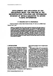
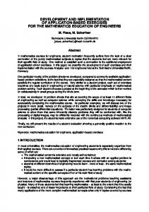
proposed by Westbrook and Dryer [53] has been employed. The combustion model which combines between a single step Arrhenius model and the Eddy-Dissipation model (EDM) via a reaction progress variable is adopted in present work due to its simplicity and inexpensive computational cost. In this work, the experimental and CFD simulation results from available literatures are required to compare. The physical conditions are given in Table 1 for the first test case based on the experiments of Akiyama et al. [56]. High pressure diesel fuel was injected into a high temperature environment in a rapid compression machine. The simulations are solved on a computational grid shown in Figure 1 with inlet SMR of 10 microns. The heat reaction rate results of two coupling models are compared as presented in Figure 2. As discussed above, before the flame appears, the turbulent mixing rate is much higher than the chemical reaction rate. The combustion equation of Model 1 is presented in Eq. (28), and Eq. (29) represents for Model 2. In Model 1, the transition between Arrhenius rate and Magnussen model is sudden, while this change is gradual in Model 2. Although the gas temperature is high enough, in Model 1, the reaction mode cannot switch until Arrhenius rate is higher than the mixing rate. As shown in Figure 2, the ignition delay time for Model 1 is then longer than for Model 2 because Model 2 can switch the mode increasingly with the higher temperature resulting in predicting auto-ignition reasonably. Furthermore, the burning rate from this coupling mode is comparable with the experimental data of Akiyama et al. [56]. This coupling reaction rate can also perform successfully in autoignition prediction as shown by Pires da Cruz et al. [54]. Hence, the transition between self-ignition and hightemperature combustion in all this work employs this coupling mode. The auto-ignition delay time in present work is based on the definition of Kang et al. [17] that the ignition delay time is the moment that the gas temperature increases rapidly. The gas temperature starts to increase sharply at around 1.8 ms as presented in Figure 3 which shows the development of gas temperature and fuel mass fraction. Thus the auto-ignition delay time for this test case is approximately 1.8 ms while the first appearance of the luminous flame in experiment of Akiyama et al. [56] is faster around 1.4 ms. The location of ignition occurs in the vapour region on the periphery of the liquid spray at around 30 mm from nozzle and 5 mm from centre line. Moreover, this ignition is located in the lean mixture zone, whereas the corresponding stoichiometric ratio with the fuel mass fraction is around 0.074. At the auto-ignition point, the fuel mass fraction is only approximately 0.04 related to a lean equivalence ratio of 0.54. This result corresponds with the simulation result of Tao et al. [57] and the DNS data of Rutland and Wang [58]. The possible reason that the ignition occurs at lean mixture locations is that these locations have experienced less evaporative cooling due to lesser liquid mass. The droplet temperature is then able to increase easily. The fast increase of gas temperature during auto-ignition is caused by heat released resulting in switching from the chemical reaction control to the turbulent mixing reaction control. After ignition took place, flame subsequently spreads around the liquid core and moves quickly downstream along the vapour region inwards to the axis of the fuel jet as presented in Figure 3. The increased gas temperature enhances the evaporation rate of liquid fuel, so that large values of fuel mass fraction appear consequently. The flame then propagates rapidly downstream until the fuel vapour downstream is all consumed resulting in the high reaction rate. During the consumption of fuel vapour, the flame becomes shorter and wider, and then it appears finally like a fireball. This simulation also corresponds with experimental results of Crue et al. [59], Bruneaux et al. [60] and Ganippa et al. [61]. Additionally, the simulated process is quite similar to the simulation results of Larsson [62] and Tao et al. [57]. At a fuel injection period of 3.0 ms, the predicted gas temperature is rather higher than of experimental results as shown in Figure 3. However, the flame shapes at 4.2 and 5.2 ms are reasonably comparable. In addition, flame distributions are also compared in term of flame area as shown in Figure 4. Occurrence of predicted flame is earlier than experimental result, and then the flame occurrence becomes closer later on. The detailed comparison of flame temperature represented in term of temperature histogram is also illustrated as in Figure 5. Comparing flame area at 4.0 and 5.0 ms after start of injection, the predicted total flame areas at specific period is nearly the same as the experimental data as shown in Figure 4, and the means of these distributions are located nearly at the adiabatic flame temperature and are also reasonably good in agreement with experimental results as presented in Figure 5. As seen, the results predicted by this model present good agreement with the experimental results at time of 4.0 and 5.0 ms after start of injection, especially the mean temperatures. The predicted average flame temperature is 1950 K at 4.0 ms, and the flame temperature continues increase until 2100 K at 5.0 ms later on. These correspond to the experimental results. However, their amplitudes of these flame distributions are quite lower than the peak values of flame area obtained from the experimental data. Although the flame areas are quite similar, large flame area appearing in these simulations present in low-temperature range, especially in spray tails. Fig. 6 shows how accurately present model can capture heat release rate. In the early stage, heat release rate slightly decreases below zero due to heating up the liquid droplets. It then rapidly increases after ignition occurs resulting in high reaction rate. Later on, the diffusion flame becomes dominant to control the reaction. The flame

approaches combustion chamber wall at time of 5.2 ms in the experiment. Hence the results after time of 5.2 ms are not considered. Comparing with the experimental results, the peak of reaction rate obtained from the experiment is higher than the peak of the simulation result. This is possible that the evaporation model employed here performs improperly at low temperature. This model can produce less fuel vapour for burning than the experimental result at low temperature leading to a lower heat release rate in early period of combustion. Later on, the simulation can generate fuel vapour properly at high temperature leading to comparable heat release rate with the experimental result in main combustion period. Principally, this combustion model is capable to capture this spray combustion experiment fairly well.

5. Conclusions The aim of this work is to develop and implement a simulation model for a spray combustion based on the spray size distribution moments introduced by Beck [34], suitable for diesel-like compression ignition engines. In the present spray model, the droplet size distribution of spray is characterized by the first four moments related to number, radius, surface area and volume of droplets, respectively. The governing equations for gas phase and liquid phase employed here are solved by the finite volume method based on an Eulerian framework. These constructed equations are based on the moment-average quantities which is the key concept for this work. The source terms of sub-models including droplet breakup, collision, evaporation, and the interactions between the liquid phase and the gas phase are derived in term of droplet moments. In the main section of this work, the sub-model employed for ignition and combustion is the coupling reaction rate between Arrhenius model and Eddy-Dissipation model (EDM) via a reaction progress variable which is widely used in combustion modelling. In addition, auto-ignition which is the onset of combustion is also investigated. The fuel library has also been modified for better predictions at high-pressure and high-temperature conditions. The simulation results obtained are also compared with the literature experimental and simulation data in order to assess the accuracy of the present model. The auto-ignition takes place in the lean fuel vapour region on the periphery of the liquid spray and subsequently spreads around the liquid core and then moves quickly downstream along the vapour region. Comparing with the experimental results, this present approach is capable qualitatively to reasonable prediction auto-ignition. In addition, the flame area developed during combustion progressed is also corresponding with the experimental data. However, the predicted results of this model seemingly present overprediction in flame temperature distributions. This might be that the sub-model of turbulence/chemistry interaction employed here is based on infinitely fast chemistry assumption. However, overall of this model is capable to predict moderately the phenomena of spray combustion.

6. References 1. 2.

Heywood, J.B., 1988, Internal Combustion Engine Fundamentals, New York, McGraw-Hill International. Halstead, M.P., Kirsch, A. and Quinn, C.P., 1977, "The Autoignition of Hydrocarbon Fuels at High temperature and Pressure – Fitting of a Mathematical Model," Combustion and Flame, Vol. 30, pp. 45-60. 3. Schäpertöns, H. and Lee, W., 1985, "Multidimensional Modelling of Knocking Combustion in S.I. Engines," SAE Technical Paper Series No. 850502. 4. Theobald, M.A. and Cheng, W.K., 1987, "A Numerical Study of Diesel Ignition," ASME Paper No. 87-FE2. 5. Kong, S.C. and Reitz, R.D., 1993, "Multidimensional Modelling of Diesel Ignition and Combustion using a Multistep Kinetics Model," ASME Paper No. 93-ICE-22. 6. Reitz, R.D. and Rutland, C.J., 1995, "Development and Testing of Diesel Engine CFD Models," Progress in Energy and Combustion Science, Vol. 21, pp. 173-196. 7. Belardini, P., Bertoli, C., Beatrice, C., D'Anna, A. and DelGiacomo, N., 1996, "Application of a Reduced Kinetic Model for Soot Formation and Burntout in Three Dimensional Diesel Combustion Computations," Proceedings of the 26th Symposium (International) on Combustion, Italy. 8. Cox, R.A. and Cole, J.A., 1985, "Chemical Aspects of the Autoignition of Hydrocarbon-Air Mixtures," Combustion and Flame, Vol. 60, pp. 109-123. 9. Hu, H. and Keck, J.C., 1987, "Autoignition of Adiabatically Compressed Combustible Gas Mixtures," SAE Technical Paper Series No. 872110. 10. Cowart, J.S., Keck, J.C., Heywood, J.B., Westbrook, C.K. and Pitz, W.J., 1990, "Engine Knock Predictions using Fully-Detailed and a Reduced Chemical Kinetic Mechanism," 23rd Symposium (International) on Combustion, The Combustion Institute, Pittsburgh, Pennsylvania.

11. Schreiber, M., Sakak, A.S., Lingens, A. and Griffiths, J.F., 1994, "A Reduced Thermokinetic Model for the Autoignition of Fuels with Variable Octane Ratings," 25th Symposium (International) on Combustion, Irvine. 12. Zhao, Z., Li, J., Kazakov, A., Zeppieri, S.P. and Dryer, F.L., 2005, "Burning Velocities and a High Temperature Skeletal Kinetic Model for n-Decane," Combustion Science and Technology, Vol. 177, pp. 89106. 13. Soyhan, H.S. and Andrae, J., 2007, "Evaluation of Kinetic Models for Autoignition of Automotive Reference Fuels in HCCI Applications," Turkish Journal of Engineering and Environmental Sciences, Vol. 31, pp. 1-8. 14. Valorani, M., Creta, F., Donato, F., Najm, H.N. and Goussis, D.A., 2007, "Skeletal Mechanism Generation and Analysis for n-Heptane with CSP," Proceedings of the Combustion Institute, Vol. 31, pp. 483–490. 15. Najt, P.M. and Foster, D.E., 1983, "Compression-Ignited Chemical Kinetic Mechanism for Hydrocarbon Fuels Homogeneous Charge Combustion," SAE Technical Paper Series No. 830264. 16. Takagi, T., Fang, C.Y., Kaminoto, T. and Okamoto, T., 1991, "Numerical Simulation of Evaporation, Ignition and Combustion of Transient Sprays," Combustion Science and Technology, Vol. 75, pp. 1-12. 17. Kang, S.H., Baek, S.W. and Choi, J.H., 2001, "Autoignition of Sprays in a Cylindrical Combustor," International Journal of Heat and Mass Transfer,, Vol. 44, pp. 2413-2422. 18. Kuo, K.K., 1986, Principles of Combustion, New York, John Wiley & Sons. 19. Tang, Q., Zhao, W., Bockelie, M. and Fox, R.O., 2007, "Multi-Environment Probability Density Function Method for Modelling Turbulent Combustion using Realistic Chemical Kinetics," Combustion Theory and Modelling, Vol. 11, pp. 889–907. 20. Kuan, T.S. and Lindstedt, R.P., 2005, "Transported Probability Density Function Modeling of a Bluff Body Stabilized Turbulent Flame," Proceedings of the Combustion Institute, Vol. 30, pp. 767–774. 21. Wright, Y.M., De Paola, G., Boulouchos, K. and Mastorakos, E., 2005, "Simulations of Spray Autoignition and Flame Establishment with Two-Dimensional CMC," Combustion and Flame, Vol. 143, pp. 402-419. 22. Klimenko, A.Y. and Bilger, R.W., 1999, "Conditional Moment Closure for Turbulent Combustion," Progress in Energy and Combustion Science, Vol. 25, pp. 595–687. 23. Burke, S.P. and Schumann, T.W., 1928, "Diffusion Flames," Proceedings of the First Symposium on Combustion, Pittsburgh, Swampscott, MA. (Reprint of Proceedings published by The Combustion institute in 1965). 24. Rakopoulos, C.D., Antonopoulos, K.A. and Rakopoulos, D.C., 2007, "Development and Application of Multi-Zone Model for Combustion and Pollutants Formation in Direct Injection Diesel Engine Running with Vegetable Oil or its Bio-Diesel," Energy Conversion and Management, Vol. 48, pp. 1881–1901. 25. Lapuerta, M., Armas, O., Ballesteros, R. and Fernandez, J., 2005, "Diesel Emissions from Biofuels Derived from Spanish Potential Vegetable Oils " Fuel, Vol. 84, pp. 773–780. 26. Cui, Y., Deng, K. and Wu, J., 2001, "A Direct Injection Diesel Combustion Model for Use in Transient Condition Analysis," Proceedings of the Institution of Mechanical Engineers, Vol. 215, pp. 995-1004. 27. Lehtiniemi, H., Mauss, F., Balthasar, M. and Magnusson, I., 2006, "Modeling Diesel Spray Ignition Using Detailed Chemistry with a Progress Variable Approach," Combustion Science and Technology, Vol. 178, pp. 1977–1997. 28. Hossain, M. and Malalasekera, W., 2005, "Numerical Study of Bluff-Body Non-Premixed Flame Structures using Laminar Flamelet Model," Proceedings of the Institution of Mechanical Engineers, Vol. 219, pp. 361370. 29. Spalding, D.B., 1970, "Mixing and Chemical Reaction in Steady Confined Turbulent Flames," The 13th Symposium (international) on Combustion, The Combustion Institute, Pittsburgh, Salt Lake City. 30. Magnussen, B.F. and Hjertager, B.H., 1976, "On Mathematical Modelling of Turbulent Combustion with Special Emphasis on Soot Formation and Combustion," in 16th Symposium (International) on Combustion, The Combustion Institute, Pittsburgh. 31. Gosman, A.D. and Harvey, P.S., 1982, "Computer Analysis of Fuel-Air Mixing and Combustion in an Axisymmetric D.I. Diesel Engine," SAE Technical Paper Series No. 820036. 32. Wang, D.M., 1992, Modelling Spray Wall Impaction and Combustion Processes of Diesel Engines, Ph.D. Thesis, Manchester, UMIST. 33. Yoong, A. and Watkins, A.P., 2004, "Modelling of LPG Spray Development, Eevaporation and Combustion," International Journal of Engine Research, Vol. 5, pp. 469-497. 34. Beck, J.C., 2000, Computational Modelling of Polydisperse Sprays without Segregation into Droplet Size Classes, Manchester, UMIST. 35. Beck, J.C. and Watkins, A.P., 2003, "The Droplet Number Moments Approach to Spray Modelling: The Development of Heat and Mass Transfer Sub-Models," International Journal of Heat and Fluid Flow, Vol. 24, pp. 242-259. 36. Beck, J.C. and Watkins, A.P., 2003, "On the Development of a Spray Model Based on Drop-Size Moments," Proceedings of the Royal Society of London, Vol. A 459, pp. 1365-1394.

37. Beck, J.C. and Watkins, A.P., 2002, "On the Development of Spray Sub-Models Based on Droplet Size Moments," Journal of Computational Physics, Vol. 182, pp. 586-621. 38. Beck, J.C. and Watkins, A.P., 2004, "The Simulation of Fuel Sprays Using the Moments of the Ddrop Number Size Distribution," International Journal of Engine Research, Vol. 5, pp. 1-21. 39. Beck, J.C. and Watkins, A.P., 2003, "The Simulation of Water and Other Non-Fuel Sprays Using a New Spray Model," Atomization and Sprays, Vol. 13, pp. 1-26. 40. Watkins, A.P., 2007, "Modelling of Mean Temperatures Used for Calculating Heat and Mass Transfer in Sprays," International Journal of Heat and Fluid Flow, Vol. 28, pp. 388-406. 41. Harlow, F.H. and Amsden, A.A., 1975, "Numerical Calculation of Multiphase Fluid Flow," Journal of Computational Physics, Vol. 17, pp. 19-52. 42. Melville, W.K. and Bray, K.N.C., 1979, "A Model of the Two-Phase Turbulent Jet," International Journal of Heat and Mass Transfer, Vol. 22, pp. 647-656. 43. Versteeg, H.K. and Malalasekera, W., 1995, An Introduction to Computaional Fluid Dynamics; The Finite Volume Method, Malaysia, Longman Scientific & Technical. 44. Mostafa, A.A. and Mongia, H.C., 1987, "On the Modelling of Turbulent Evaporating Sprays: Eulerian versus Lagrangian Approach," International Journal of Heat and Mass Transfer, Vol. 30, pp. 2583-2593. 45. Launder, B.E. and Spalding, D.B., 1972, Lectures in Mathematical Models of Turbulence, London, Academic Press. 46. Beck, J.C., 2000, Computational Modelling of Polydisperse Sprays without Segregation into Droplet Size Classes, Ph.D. Thesis, Manchester, UMIST. 47. Nicholls, H., 1972, "Stream and Droplet Breakup by Shockwaves," NASA SP-194, Eds. Harrje and Reardon, pp.126-128. 48. Faeth, G.M., Hsiang, L.P. and Wu, P.K., 1995, "Structure and Break-Up Properties of Sprays," International Journal of Multiphase Flow, Vol. 21, pp. 99-127. 49. O’Rourke, P.J. and Bracco, F.V., 1980, " Modelling of Drop Interactions in Thick Sprays and a Comparison with Experiments," Conference on Stratified Charge Automotive Engines, No. C404/80, Institute of Mechanical Engineers (IMechE). 50. Orme, M., 1997, "Experiments on Droplet Collisions, Bounce, Coalescence and Disruption " Progress in Energy Combustion Science, Vol. 23, pp. 65-79. 51. Qian, J. and Law, C.K., 1997, "Regimes of Coalescence and Separation in Droplet Collision," Journal of Fluid Mechanics, Vol. 331, pp. 59-80. 52. Wallis, G.B., 1969, One-Dimensional Two-Phase Flows, New York, McGraw-Hill. 53. Westbrook, C.K. and Dryer, F.L., 1984, "Chemical Kinetic Modelling of Hydrocarbon Combustion," Progress in Energy and Combustion Science, Vol. 10, pp. 1-57. 54. Pires da Cruz, A., Baritaud, T.A. and Poinsot, T.J., 2001, "Self-Ignition and Combustion Modeling of Initially Nonpremixed Turbulent Systems," Combustion and Flame, Vol. 124, pp. 65-81. 55. Issa, R.I., 1986, "Solution of the Implicitly Discretised Fluid Flow Equations by Operator-Splitting," Journal of Computational Physics, Vol. 62, pp. 40-65. 56. Akiyama, H., Nishimura, H., Ibaraki, Y. and Iida, N., 1998, "Study of Diesel Spray Combustion and Ignition using High-Pressure Fuel Injection and a Micro-Hole Nozzle with a Rapid Compression Machine: Improvement of Combustion using Low Cetane Number Fuel," Society of Automotive Engineers of Japan, Vol. 19, pp. 319-327. 57. Tao, F., Golovitchev, V.I. and Chomiak, J., 2001, "Application of Complex Chemistry to Investigate the Combustion Zone Structure of DI Diesel Sprays under Engine-Like Conditions," The Fifth International Symposium on Diagnostics and Modeling of Combustion in Internal Combustion Engines (COMODIA 2001), Nagoya. 58. Rutland, C.J. and Wang, Y., 2006, "Turbulent Liquid Spray Mixing and Combustion – Fundamental Simulations," Journal of Physics, Vol. 46, pp. 28-37. 59. Crua, C., Kennaird, D.A., Sazhin, S.S. and Heikal, M.R., 2004, " Diesel Autoignition at Elevated InCylinder Pressures," International Journal of Engine Research, Vol. 5, pp. 365-374. 60. Bruneaux, G., Augé, M. and Lemenand, C., 2004, "A Study of Combustion Structure in High Pressure Single Hole Common Rail Direct Diesel Injection Using Laser Induced Fluorescence of Radicals," The Sixth International Symposium on Diagnostics and Modeling of Combustion in Internal Combustion Engines, (COMODIA 2004), Yokohama, Japan. 61. Ganippa, L.C., Andersson, S. and Chomiak, J., 2003, "Combustion Characteristics of Diesel Sprays from Equivalent Nozzles with Sharp and Rounded Inlet Geometries," Combustion Science and Technology, Vol. 175, pp. 1015-1032. 62. Larsson, A., 1999, "Optical Studies in a DI Diesel Engine," SAE Technical Paper Series No. 1999-01-3650.

Table 1 The physical conditions of spray injection test cases. Fuel Time step (µs) Injection cell of largest side (mm) Cell grid (z×r cells) Inlet SMR (µm) Trap pressure (MPa) Maximum injection pressure (MPa) Trap temperature (K) Liquid temperature (K) Injector diameter (mm) Injection duration (ms) Fuel Injection quantity (mg)

Diesel (CN 55) 0.5 0.5 109x73 10.0 2.7 80.0 830 298 0.18 3.8 28.0

0.03

Y

0.02

0.01

0

0

0.05

0.1 X

0.15

0.2

Figure 1 Grid used for all cases in the spray combustion. The domain is 200 mm long and 30 mm in radius with 109x73 cells

Burning rate (microgram/ms) .

35000 Model 1; B=4 Model 1; B=8 Model 1; B=12 Model 1; B=inf Model 2; B=4 Model 2; B=5 Model 2; B=6

30000 25000 20000 15000 10000 5000 0 0

2

4

6

8

Time after injection (ms) Figure 2 Time history of burning rate at different model for test case. (Model 1: ω = min(ωc, ωt); Model 2: ω = ωc(1-c)+ωtc; where ωc = 3.2 × 1011 ρYF0.25YO1.50 exp(−15100 / T ) ; ω = Bρ ε min(Y , YO , YP ) ) t F k

s 1+ s

10

Time

1.8 ms

3.0 ms

4.2 ms

5.2 ms

Gas temperature

Fuel vapour mass fraction

Flame Luminosity [56]

Figure 3 The contour of gas temperature and fuel vapour mass fraction comparing with the experiment results of Akiyama et al. [56]

3000

Flame area (mm2)

2500 2000 1500 1000

Experimental data Predicted data

500 0

2

2.5

3

3.5

4

4.5

5

Time after injection (ms) Figure 4 Development of flame area for the experiment of Akiyama et al. [56]

5.5

2000 Exp. (5.0 ms ASI)

1800

Sim. (5.0 ms ASI)

Flame area (mm2)

1600

Exp. (4.0 ms ASI)

1400

Sim. (4.0 ms ASI)

1200 1000 800 600 400 200 0 1400

1600

1800

2000

2200

2400

2600

2800

Flame temperature (K) Figure 5 Comparing flame temperature histogram for experiment of Akiyama et al. [56] at 4.0 and 5.0 ms after start of injection.

900

Heat released rate (J/ms)

800 700 Predicted data Experimental data

600 500 400 300 200 100 0 -100

0

2

4

6

8

10

Time after injection (ms) Figure 6 Time history of heat release rate for the experiment of Akiyama et al. [56]