Aerosol Science and Technology, 37:804–817, 2003 c American Association for Aerosol Research Copyright ° ISSN: 0278-6826 print / 1521-7388 online DOI: 10.1080/02786820390223963
Development and Validation of a Simple Numerical Model for Estimating Workplace Aerosol Size Distribution Evolution Through Coagulation, Settling, and Diffusion Andrew D. Maynard and Anthony T. Zimmer National Institute for Occupational Safety and Health, Cincinnati, Ohio
Recent research has indicated that the toxicity of inhaled ultrafine particles may be associated with the size of discrete particles deposited in the lungs. However, it has been speculated that in some occupational settings rapid coagulation will lead to relatively low exposures to discrete ultrafine particles. Investigation of likely occupational exposures to ultrafine particles following the generation of aerosols with complex size distributions is most appropriately addressed using validated numerical models. A numerical model has been developed to estimate the size-distribution time-evolution of compact and fractal-like aerosols within workplaces resulting from coagulation, diffusional deposition, and gravitational settling. Good agreement has been shown with an analytical solution to lognormal aerosol evolution, indicating good compatibility with previously published models. Validation using experimental data shows reasonable agreement when assuming spherical particles and coalescence on coagulation. Assuming the formation of fractal-like particles within a range of diameters led to good agreement between modeled and experimental data. The model appears well suited to estimating the relationship between the size distribution of emitted well-mixed ultrafine aerosols, and the aerosol that is ultimately inhaled where diffusion loses are small.
INTRODUCTION Occupational aerosol exposure has traditionally been characterized by the mass concentration of particles within welldefined size ranges (CEN 1993; ISO 1995). However, recent research has indicated that for a number of low-solubility materials the number, size, and surface area of particles depositing in the lungs may all play a significant role in determining adverse health effects (Donaldson et al. 2000; Oberd¨orster 2000). Much of the resulting discussion has focused on ultrafine particles— nominally particles with a diameter smaller than 100 nm. For
Received 23 July 2002; accepted 19 March 2003. Address correspondence to Andrew D. Maynard, National Institute for Occupational Safety and Health, 4676 Columbia Parkway, Cincinnati, OH 45226, USA. E-mail:
[email protected]
804
instance, research using polystyrene latex, PTFE, and TiO2 particles has indicated lung deposition of ultrafine particles leads to a greater biological response than a similar mass of much larger particles (Oberd¨orster 2000). It has been suggested that the observed response is due to the increased available surface area associated with the ultrafine particles. An alternative hypothesis is that biological response is associated with particle number, possibly due to particle penetration through the interstitium into the bloodstream (Seaton et al. 1995; Nemmar et al. 2002). However, this hypothesis assumes that a substantial number of discrete ultrafine particles will deposit in the lungs following exposure. In many workplaces the number concentration of generated ultrafines is likely to reach sufficiently high concentrations to lead to rapid coagulation: In this case it may be hypothesized that the number concentration of particles below 100 nm being inhaled will be relatively small (Vincent and Clement 2000). Many workplaces also contain a range of aerosol sources, and it is conceivable that scavenging by large particles will lead to relatively few ultrafine particles being available for inhalation. If the number concentration of discrete ultrafine particles entering the respiratory system is associated with toxicity, the persistence of particles within the ultrafine region between generation and inhalation becomes a critical factor in determining associated health risks. Estimates of ultrafine particle removal through coagulation from lognormal distributions are calculable analytically (Park et al. 1999). However, this approach is inappropriate where the distribution is not well characterized by a lognormal distribution, and in particular where it is multimodal. In the case of complex particle size distributions, numerical modeling provides a more appropriate method of estimating particle persistence through predicting the time-evolution of an aerosol. The use of numerical routines for modeling spatial and temporal aerosol dynamics is well established, and represented by an extensive literature (Kommu et al. (2002) provide an extensive review of methods). However, there is a lack of published information on validated models appropriate to understanding the temporal evolution of ultrafine aerosols in the workplace.
805
COAGULATION OF WORKPLACE AEROSOLS
A relatively simple discrete numerical model has been developed to consider the temporal evolution of workplace-related aerosols extending into the ultrafine region. By assuming wellmixed “parcels” of aerosol travel between the source and the point of inhalation at a known velocity, the need for a spatial component within the model has been removed (it is assumed that the parcel volume is large compared to inhaled aerosol volume). The model is further simplified by restricting it to physical processes assumed to dominate the behavior of ultrafine particles released into a workplace environment—these being generation, coagulation, and deposition through settling and diffusion. No account has been made of nucleation and condensation, restricting the model to the point beyond which these processes become secondary to coagulation and deposition processes. Validation of the model has been carried out using an aerosol generated during high speed grinding, thus representing a multimodal occupational aerosol spanning several orders of particle diameter (Zimmer and Maynard 2002). The model was developed and run within the software package Mathematica°R (Wolfram Research Inc., Champagne, IL). MODEL
Coagulation Smoluchowski theory (Smoluchowski 1917) describing the thermal coagulation of spherical particles in an initially monodisperse distribution has been used extensively and effectively as the basis for predicting coagulation-mediated size distribution evolution. Extending the theory to a polydisperse distribution gives the change in concentration of particles with mass m with time as 1 dn(m) = dt 2
Z
m
n(m 1 )K (m 1 , m − m 1 )n(m − m 1 )dm 1 Z ∞ − n(m) K (m, m 1 )n(m 1 )dm 1 [1] 0
0
(Fuchs 1964). K is the coagulation coefficient describing the probability of coagulation between particles of mass m and m 1 . For particles in the continuum region coagulation coefficient, K 0 is given by the standard expression µ K 0 (m, m 1 ) = 4π
d(m) + d(m 1 ) 2
¶µ
¶ D(m) + D(m 1 ) , [2] 2
where d(m) is the diameter of a particle with mass m, and D(m) is the diffusion coefficient of the particle. As particle size enters the free molecular regime, assumptions leading to Equation (2) begin to break down. The Fuchs correction factor β extends the usefulness of Equation (2) through the transition regime into the free molecular regime, giving the coagulation coefficient K as K = β K0,
[3]
where µ β=
d πλp +√ d +δ 2d
¶−1 [4]
λ p is the particle mean free path. The factor δ is given by ½
√ δ= 2
· ¸ ¾ ¡ 2 ¢3 1 3 2 2 (d + λ p ) − d + λ p −d 3dλ p
[5]
(Fuchs 1964). Equations (1) and (3) allow coagulation to be modeled between particles of a few nanometers in diameter to tens of micrometers in diameter and are well suited to numerical modeling.
Loss Rate The rate of particle loss through gravitational settling assuming continuous mixing may be expressed as ¯ n(m)vts dn(m) ¯¯ , [6] =− ¯ dt settling h where h is a characteristic height of the modeled system and vts is the particle settling velocity. Diffusional losses are more complex to include. In an open environment it may be assumed that equivalent cells surround the aerosol cell being modeled, and thus the outward diffusional flux is matched by an equivalent inward flux. However, where the cell is bounded by solid surfaces, some account needs to be taken of diffusional losses to these surfaces. Assuming continuous mixing of the aerosol, the rate of particle loss through diffusion is given as ¯ An D dn(m) ¯¯ =− , [7] dt ¯wall losses V δdiff where A is the total surface area of deposition surfaces bounding the aerosol, V the bounded aerosol volume, and δ diff the diffusion boundary layer depth at the surfaces. δ diff is a function of particle diameter and air movement at the boundary and is not simply represented analytically. For complex geometries there is interaction between gravitational and diffusional deposition, and Equations (6) and (7) have been found to be inadequate in representing deposition rates. (Crump et al. 1983). However, for rectangular enclosures with vertical walls their use is appropriate (Crump and Seinfeld 1981). Wells and Chamberlain (1967) have shown δ diff to be proportional to D 1/3 for simple geometries, while Crump and Seinfeld (1981) suggest it to be approximately proportional to D 1/2 in a cubic geometry. For this case an approximation of the diffusion layer depth may therefore be given by δdiff = k D β ,
[8]
where k is an empirically determined constant that is dependent on the geometry and conditions being modeled. β is expected to lie between 1/2 and 1/3.
806
A. D. MAYNARD AND A. T. ZIMMER
In the model it was assumed that the aerosol was at charge equilibrium, and that electrostatic forces would have a secondary influence over coagulation and deposition. These assumptions appeared to satisfy the model validation against the experimental data in this case. However, in some workplaces an extension of the model to include electrostatic effects would undoubtedly be advantageous. Combining Equations (1), (6), and (7) and adding terms describing aerosol dilution and particle generation gives the rate of change of particle concentration with time as Z 1 m dn(m) = n(m 1 )K (m 1 , m − m 1 )n(m − m 1 )dm 1 dt 2 0 Z ∞ n(m)vts − n(m) K (m, m 1 )n(m 1 )dm 1 − h 0 An(m)D − − 0n(m) + S, [9] V δdiff where 0 is the fractional dilution rate and S is a source term. Equation (9) is used as the basis of the numerical model described here. An initial aerosol size distribution is described in terms of a series of discrete particle mass bins, with the number of particles in each bin representing particle number concentration between the upper and lower bin limits. A geometric series is used to define the mass bin series at time t = 0. dn | is initially calculated within the model for each bin dt t=0 using the geometric midpoint particle mass, and the discrete form of Equation (9). Using this approach directly, mass is not conserved. The formation rate of particles with mass m k due to coagulation of particles with masses m i and m j is therefore adjusted to conserve mass using the relationship ¯ dn(m k ) ¯¯ dt ¯coag. growth, adjusted ¯ mi + m j dn(m k ) ¯¯ = × [10] dt ¯ m coag. growth
k
(Gentry and Cheng 1996). Aerosol mass is subsequently conserved in the modeled evolving size distribution.
Time Progression An initial estimate of number concentration at time t + 1t is given by ¯ dn ¯¯ [11] n(t + 1t) = n(t) + ¯ × 1t. dt t This approximation is useful in estimating a suitable value of 1t, and is used within the model to estimate 1t such that no bin is depleted by more than 50%, or increased by 100%. Although these limits are arbitrary, they effectively reduce potentially catastrophic extrapolation errors associated with very large values of 1t. The implicit assumption of Equation (11) is that for a sufficiently small value of 1t higher order derivatives of
n(t) are insignificant. A more precise estimate of n(t + 1t) can be made using a Taylor expansion: ¯ i X 1 d m n ¯¯ n(t + 1t)i = n(t) + × 1t m , [12] m ¯ m! dt t m=1 where i represents the ith estimate of n(t + 1t), although calculating successive derivatives becomes increasingly computationally intensive. A computationally efficient solution is to between t iteratively improve estimates of the mean value of dn dt and t + 1t using µ ¯ ¶ 1t dn ¯¯ d + n(t + 1t)i−1 . [13] n(t + 1t)i = n(t) + 2 dt ¯t dt Successive iterations of Equation (13) approximate to ¯ i X 1 d m n ¯¯ × 1t m . n(t + 1t)i = n(t) + m−1 dt m ¯ 2 t m=1
[14]
Using Equation (14), estimates of n(t + 1t) may be iteratively improved until X
n i+1 (t + 1t) −
d
X
n i (t + 1t) ≤ n lim ,
[15]
d
where n lim is a preset convergence point. Equation (14) initially approximates the Taylor expansion well, although ultimately it does not converge. However, it is not a precise representation of Equation (13), and in practice successive estimates of n(t + 1t) were found to converge rapidly. The model as described thus far is limited by the somewhat arbitrary constraints on the initial selection of 1t. A more reasonable approach is to select 1t to ensure that the difference between successive estimates of n(t + 1t)i are within acceptable bounds (defined by 1n min and 1n max ). If it is assumed that n(t + 1t) is well represented by the first three terms of the Taylor expansion, then the difference between the first and second order estimates of n(t + 1t), denoted 1n 1,2 , is given by 1n 1,2 = 2
1 d 2n 2 1t . 2 dt 2
[16]
By evaluating ddt n2 , 1t may be re-estimated to give 1n 1,2 within the preset bounds when it lies outside the range 1n min → 1n max . Using this method, the maximum value of 1t is still restricted to that which will lead to no bin being depleted by more than a set percentage to prevent negative number concentrations. This criterion becomes particularly restrictive as bins experiencing are depleted to the point of containing high negative values of dn dt negligible particles, resulting in the modeled size distribution evolution being dominated by bins that represent an insignificant fraction of the whole distribution. Selecting 1t to deplete these bins by exactly 100% would solve this problem. However, the
807
COAGULATION OF WORKPLACE AEROSOLS
method used to iteratively improve the estimate of n(t + 1t) cannot be guaranteed to lead to precisely 100% depletion in a key bin. The solution within the model is to merge bins together that contained restrictively small numbers of particles, ensuring that 1t remains within acceptable limits.
Adaptive Bin Widths—Bin Merging Following the final estimation of n(t + 1t), the value of 1t is estimated for each bin that will lead to 50% depletion after between t and the next time step (based on the mean value of dn dt t +1t). Bins where 1t is less than a preset target value (1t target ) are merged with neighboring bins. Resulting upper and lower bin limits are calculated to conserve particle number and mass. Three regimes for bin merging are identified: bins adjacent to and including the lowest bin in the series (low regime), bins adjacent to and including the highest bin (high regime), and bins or series of bins bordered by nontagged bins on either side (middle regime) (Figure 1). For each, a different merging algorithm is used. Middle Regime. Following merging, the lower edge of the first bin (m j−1 ) is equivalent to m i−1 , and the upper edge of the second bin (m j+1 ) is equivalent to m i+2 (Figure 1). The particle number in each resulting bin is set to 1 n j−1 = n i−1 + n i , 2 1 n j = n i+1 + n i . 2
[17]
The lower edge of the upper bin following merging (m j ) is calculated to conserve mass, giving µ ¶ √ √ √ n i−1 m i−1 m i + n i m i m i+1 + n i+1 m i+1 m i+2 2 . mj = √ √ n j−1 m i−1 + n j m i+2 [18] Lower Regime. Following merging, the particle number in the resulting bin (n j ) is equal to n j = n i + n i+1
[19]
(Figure 1). The upper edge of the resulting bin is set to be the same as the upper edge of the adjacent bin (m i+2 ), giving the lower edge of the resulting bin (m j ) as µ √ ¶ √ n i m i m i+1 + n i+1 m i+1 m i+2 2 . mj = √ n j m i+2
[20]
upper edge of the resulting bin (m j+1 ) as µ m j+1 =
¶ √ √ n i−1 m i−1 m i + n i m i m i+1 2 . √ n j m i−1
[22]
For each regime the above algorithms are sequentially repeated for each tagged bin.
Solid Particle Coagulation—Inclusion of Fractal Dimension The model as described up to this point assumes spherical particles and coalescence on coagulation, and thus is only strictly applicable to liquid aerosols. Coagulation of solid particles tends to form fractal-like agglomerates, which exhibit a behavior that is associated with their structure. There is an extensive literature on the formation and behavior of fractal-like aerosol agglomerates (e.g., Forrest and Witten, Jr. 1979; Schmidt-Ott 1988; Hagenloch and Friedlander 1989; Jiang and Logan 1991; Rogak et al. 1993; Wu and Friedlander 1993; Baron et al. 2001). However, an approach to formulating a general numerical coagulation model spanning the free molecular regime to the continuum regime is not immediately clear. Brownian coagulation is largely governed by particle diffusional mobility and effective collision diameter. In the case of spherical particles, mobility diameter and collision diameter can be assumed to be similar. However, this assumption breaks down for fractal-like agglomerates. Hagenloch and Friedlander (1989) have proposed that dcl ≈ Nα d0
[23]
for Knudsen number Kn > 1, where dcl is the particle collision diameter, d0 the primary particle diameter, and N the number of primary particles in the agglomerate. α → 0.45 as Kn → ∞ for a fractal dimension D f of 2.5. Equation (23) may be approximated as µ ¶D f df [24] N= d0 (Rogak et al. 1993), where d f is the agglomerate’s outer diameter. If d f is assumed to be equivalent to dcl , Equation (24) leads to α = 0.4 for D f = 2.5—a close approximation to Hagenloch and Friedlander. If d0 and primary particle density ρ are known for an agglomerate of mass m, N is calculable, and dcl can be estimated from Equation (24) as 1
Upper Regime. given by
Particle number in the merged bin (n j ) is n j = n i + n i−1
[21]
(Figure 1). The lower edge of the resulting bin is set to be the same as the lower edge of the adjacent bin (m i−1 ), giving the
dcl ≈ d f = d0 N D f .
[25]
The mobility diameter (dm ) of agglomerates with D f < 2 has been shown to be equivalent to the equivalent-sphere projectedarea diameter d A (Rogak et al. 1993). For D f < 2 most of the primary particles in an agglomerate are exposed, and the projectedarea can be assumed to be equivalent to the orientation-averaged
808
A. D. MAYNARD AND A. T. ZIMMER
Figure 1. Schematic representation of algorithms used to merge mass bins when the particle number in a given bin is sufficiently low to lead to excessively short time steps. area of a straight chain with the same N (Rogak et al. 1993). Thus √ 1 d0 dm ≡ d A = √ [(1 + N )π 2 + 4(3 3 − 4)(N − 1)] 2 . [26] 2π
correction factor β is estimated from the effective collision diameter of particles. Substituting dm for d in Equation (2) and d f for d in Equations (4) and (5) gives
Coagulation coefficient K 0 is dependent on the relative diffusion rate between particles, and therefore may be effectively estimated using particle mobility diameter. However, the Fuchs
K 0, fractal (m, m 1 ) = 4π
µ
dm (m) + dm (m 1 ) 2
¶µ
¶ D(m) + D(m 1 ) 2 [27]
COAGULATION OF WORKPLACE AEROSOLS
and
¶−1
df πλ p +√ , d f + δfractal 2d f ½ ¾ √ ¡ ¢3 i 1 h = 2 (d f + λ p )3 − d 2f + λ2p 2 − d f , 3d f λ p [28]
βfractal = δfractal
µ
with K fractal = βfractal K 0, fractal ,
[29]
allowing the coagulation model to be extended to fractal agglomerates with D f ≤ 2. The diffusion coefficient D in Equation (27) is clearly evaluated using dm . Equation (29) becomes equivalent to Equation (3) for D f = 3, allowing it to be used for compact and fractal-like particles. Wu and Friedlander (1993) have addressed the same problem starting from the free molecular regime expression for K , using similar assumptions. Their final expression for K fractal gives values that agree well with Equation (29). However, their expression is only of use for Kn > 10 and D f > 2, and thus was not used within the numerical model.
809
While Equation (29) allows the growth of fractal-like aerosols to be modeled effectively, it is unrealistic to assume all particles within an aerosol will have the same fractal dimension. In the simplest terms, it may be assumed that particle morphology is driven by generation mechanism, with fine particles tending towards a fractal-like geometry, and coarse particles tending towards a compact geometry. This assumed tendency is incorporated into the model as a step function defining D f —particles smaller than a limiting diameter (dlimit ) are assumed to be fractallike (when modeling solid particle behavior), while particles larger than dlimit are assumed to be spherical. Although this is an oversimplification, it allowed effective comparison with experimental data. The model also assumes that particles smaller than the primary particle size are spherical. MODEL VALIDATION
Comparison with an Existing Analytical Model Initial validation of the discrete numerical model was carried out against an analytical model describing the coagulation of lognormal aerosol size distributions for the entire particle
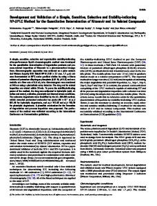
Figure 2. Plotting normalized particle number concentration versus dimensionless time for the analytical lognormal coagulation model of Park et al. (1999) and the numerical coagulation model. K co is the coagulation coefficient in the continuum regime.
810
A. D. MAYNARD AND A. T. ZIMMER
size range (Park et al. 1999). The Park et al. analytical model has been compared favorably with both sectional and discrete numerical models (Otto et al. 1999), making it particularly suitable for validating new code. Comparisons were made between the time-evolution of three lognormal distributions, representing coagulation in the free-molecular regime (Count Median Diameter (CMD)) = 1 nm, the transition regime (CMD = 100 nm), and the continuum regime (CMD = 1 µm). In each case the geometric standard deviation was 1.6, and the number concentration 1012 particles/m3 . The time-evolution of each distribution was modeled for between 20,000 s and 100,000 s in each case. Figure 2 compares normalized number concentration against dimensionless time for each distribution. In each case very close agreement between the discrete numerical model and the analytical model is seen. Size distributions for the transition-regime aerosol are plotted in Figure 3 for each model. The discrete model appears to slightly underestimate number concentration close to the median diameter, and overestimate it towards the
edges of the distribution. However this is most likely an artifact of using discrete size bins. Overall the agreement between both models is very close.
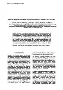
Validation Against Experimental Data Experimental Method. Experimental validation of the numerical model was carried out by measuring the temporal size distribution evolution of polydisperse aerosols spanning over three decades of particle diameter. The aerosols were generated through high-speed grinding of a series of substrates—a method previously shown to generate particles from a few nanometers in diameter up to tens of micrometers in diameter (Zimmer and Maynard 2002). The generation method used was identical to that described by Zimmer and Maynard. HEPA-filtered, particle-free air was pulled upward through a stainless steel chamber (approximately 1 m3 ) (Figure 4). Prior to measurements, the HEPA-filtered air within the chamber was monitored using a condensation particle counter (CPC) (TSI Inc., Model 3022A, Shoreview, MN). When
Figure 3. Comparison of the numerical model and the Park et al. (1999) analytical lognormal model for an initial lognormal aerosol distribution with CMD = 100 nm, σg = 1.6, and number concentration = 1012 particles/m3 .
COAGULATION OF WORKPLACE AEROSOLS
Figure 4. Schematic of the experimental aerosol generation and sampling system (not to scale). the particle number concentration was reduced to a value of approximately 50 × 106 particles/m3 , the air flow was stopped, and the chamber sealed. Concentrations below this were not achievable due to some infiltration into the chamber. A small, tubeaxial fan (Pamotor, Model 8500C, Burlingame, CA), located within the base of the chamber, was used to create “stirred” conditions (CPC measurements validated that the fan did not represent a source of aerosols). Grinding was carried out using a Dremel MultiproTM (Model 395, Racine, WI), a variable-speed tool with rotational speeds that can be varied from 5000 to 30000 revolutions per minute (rpm). A cylindrical aluminum oxide grinding wheel was selected for these experiments. The rotational speed of the grinding wheel set at approximately 20,000 rpm in each case. Grinding was accomplished such that the cylindrical wheel was placed normal to the substrate with a constant applied force of 3.96 N. The substrates selected for grinding included aluminum, polytetrafluoroethylene (PTFE), and granite. Aerosol samples were collected from the chamber at a position located directly above the grinding operation (height = 0.15 m). The aerosol-laden air collected from the chamber was split and directed to one of three aerosol instruments operated in parallel. The smallest particles (4.22 nm < dm < 100 nm) were characterized using a scanning mobility particle sizer (SMPS) configured with a nano differential mobility analyzer (DMA) (TSI Inc., an Electrostatic Classifier, Model 3080, using a Nano Differential Mobility Analyzer, Model 3085, and a Condensation Particle Counter (CPC), Model 3022A, St. Paul, MN). Larger particles (60.4 nm < dm < 777 nm) were characterized using a SMPS configured with a long DMA (TSI Inc., DMA Model 3934 and CPC Model 3022A, St. Paul, MN). The largest
811
particles (523 nm < aerodynamic diameter dae < 20.5µm) were characterized using an aerodynamic particle sizer (APS) (TSI Inc., Model 3320). Particle number concentrations detected by each instrument were sufficiently low to lead to significant overload or coincidence errors. The overall sampling flow rate to the three instruments was 1.6 l/min. To minimize aerosol extraction from the chamber, instruments were disconnected from it between samples being taken. Rogak et al. (1993) have shown particle mobility diameter to agree well with equivalent-sphere projected-area diameter for fractal-like particles below 1 µm. The assumption was therefore made that the data from each SMPS could be interpreted in terms of particle equivalent-sphere projected-area diameter. Particles large enough to be sampled by the APS were assumed to arise predominantly through attrition, and have a compact morphology. APS aerosol size distributions were therefore transformed to particle number concentration versus equivalent sphere projected-area diameter assuming spherical particles with the same density as the bulk substrate material. The APS data were also corrected for sampling train losses between the chamber and the instrument inlet, and losses within the APS nozzle (Kinney and Pui 1995). Calculations indicated sampling train losses to each SMPS to be negligible. Low concentration aerosols of PTFE and granite were generated to investigate particle deposition through diffusion and gravitational settling, in the absence of significant coagulation. In each case the substrate was ground for 10 s, and the aerosol allowed to fully mix within the chamber for 60 s. prior to sampling. Size distribution measurements were then taken at intervals over the next 2–4 h, with each measurement taking 200 s. To increase the aerosol concentration sufficiently for coagulation to play a significant role, the aluminum substrate was ground continuously until a stable size distribution was obtained. At this point three consecutive distribution measurements were made over a period of 10 min to ensure the distribution was stable prior to starting the time series measurements. Although there were small variations in the distribution with time, these were considered insignificant. The average of the three initial measured distributions was taken to represent the aerosol size distribution at t = 0 s. Size distribution measurements were then taken at 500 s, 1500 s, and 4500 s following termination of grinding, with each sample lasting 200 s. Over the course of the sampling period, 5% of the air within the chamber was removed by the sampling instruments. Replenishment of sampled air with clean air during experimental measurements was modeled using the dilution term in Equation (9). Comparison with Model. Experimental data for all substrates indicated very broad polydisperse distributions. Data from each instrument agreed well in the overlap regions, allowing a continuous distribution between 4 nm and 20 µm to be measured in each case. With the low particle concentrations from the granite and PTFE substrates (total particle concentrations