Development and Validation of Generalized Lifting Line Based Code ...

Development and Validation of Generalized Lifting Line Based Code for Wind Turbine Aerodynamics F. Grasso A. van Garrel J.G. Schepers

January 2011 ECN-M--11-004

Paper presented at “49th AIAA Aerospace Sciences Meeting, 30th ASME Wind Energy Symposium”, Orlando, FL., USA, 4-7 January 2011

Development and Validation of Generalized Lifting Line Based Code for Wind Turbine Aerodynamics F. Grasso1, A. van Garrel2 and G. Schepers3 Energy Research Centre of the Netherlands (ECN), 1755 LE, Petten, The Netherlands In order to accurately model large, advanced and efficient wind turbines, more reliable and realistic aerodynamic simulation tools are necessary. Most of the available codes are based on the blade element momentum theory. These codes are fast but not well suited to properly describe the physics of wind turbines. On the other hand, by using computational fluid-dynamics codes, in which full Navier-Stokes equations are implemented, a strong expertise and a lot of computer time to perform analyses are required. A code, based on a generalized form of Prandtl’s lifting line in combination with a free wake vortex wake has been developed at Energy research Centre of Netherlands. In the present work, the development of this new code is presented, together with the results coming from numericalexperimental comparisons. The final part of the work is dedicated to the analysis of innovative configurations like winglets and curved blades.

Nomenclature α αi c cj dF dl dSi φr Γ L r0 r1 r2 ρ uai uni u v V V∞ vij ω w 1

= = = = = = = = = = = = = = = = = = = = = = =

angle of attack [deg] local angle of attack for wing section i [deg] chord [m] chord for wing section j [m] differential aerodynamic force vector directed differential vortex length vector differential planform area at control point i azimuth angle [deg] vortex strength in the direction of r0 [m2 s-1] Lift [N] vector from beginning to end of vortex segment vector from beginning of vortex segment to arbitrary point in space vector from end of vortex segment to arbitrary point in space fluid density [kg m-3] chordwise unit vector at control point i normal unit vector at control point i axial component local velocity [m s-1] in plan horizontal component local velocity [m s-1] local fluid velocity [m s-1] velocity of the uniform flow or free stream [m s-1] dimensionless velocity induced at control point j by vortex i , having a unit strength vortex strength [ s-1] in plan vertical component local velocity [m s-1]

Postdoctoral Aerodynamicist, Wind Energy Unit, Rotor and Wind Farms Aerodynamics Group, Westerduinweg 3; [email protected], Associate Fellow AIAA 2 Senior Aerodynamicist, Wind Energy Unit, Rotor and Wind Farms Aerodynamics Group, Westerduinweg 3; [email protected] 3 Senior Aerodynamicist, Wind Energy Unit, Rotor and Wind Farms Aerodynamics Group, Westerduinweg 3; [email protected]

I

I.

Introduction

N order to design more advanced and efficient wind turbines, more accurate results coming from numerical

predictions are mandatory. This need became more and more important in the last years due to the growth of wind turbines, especially for offshore scenarios. The diameter of a modern MW class wind turbine can easily be greater than 100m, on which the effect of wind shear and incoherent atmospheric structures on blade loads play a much more significant role. Most of the available codes are based on Blade Element Momentum (BEM) theory [1, 2]. The main advantage of this class of codes is the fact that they are very fast to calculate the loads and performance of a wind turbine. This makes BEM codes very convenient especially in the very extensive wind turbine design and load calculations, but due to all the hypotheses of the theory, there are several restrictions for BEM codes usage. From the geometrical point of view for example, it is not possible to model winglets or sweep-back blades. From the aerodynamic point of view, the effects of e.g. yaw, three-dimensional rotational and geometric effects, non-stationary effects and stall are modeled with correcting factors. Investigations related with three-dimensionality of the flow, boundary layer, pressure distribution along the blade and wake-connected phenomena are not possible by using this approach. For these purposes, more complex formulations should be used. By using full Navier-Stokes based codes, for example, there are no limitations about the geometry and no restrictive hypotheses related with the aerodynamics, so it is possible to perform both detailed fluid-dynamics studies and general performance-oriented analyses in very general conditions. The drawback is the big demand in terms of computational resources, computational time and expertise. A code, named Aerodynamic Windturbine Simulation Module (AWSM), has been developed at Energy research Centre of the Netherlands (ECN) by van Garrel [3]. The main scope was to keep the advantages of BEM codes in terms of calculation time and ease of use, but to obtain a superior quality, especially concerning wake and time dependent wake-related phenomena. In the next section, the mathematical formulation is presented; then the results from the validation tests are illustrated and discussed.

II.

AWSM code

The AWSM code [3-5] is based on generalized lifting line theory in combination with a free vortex wake method. The main assumption in this theory is that the extension of the geometry in span-wise direction is predominant compared to the ones in chord and thickness direction; because of this, the real geometry is represented

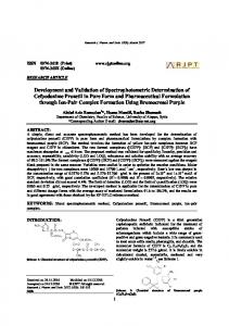
with a line passing through the quarter chord point of each cross section and all the flow field in chord-wise direction is concentrated in that point (Fig. 1).

Fig. 1 Flowfield model. Considering the elementary force (dF) generated by the geometry, this can be calculated by using the threedimensional form of the Kutta-Jukowsky equation (eq. 1).

r r r d F = ρΓ V × d l

(1)

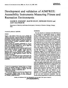
For each point along the lifting line, the local velocity Vi can be calculated as superimposition of local free stream velocity and local induced velocity (eq. 2), where vij is the dimensionless induced velocity calculated from Biot-Savart formula (eq. 3, according to the nomenclature used in Fig. 2).

Fig. 2 Position vectors describing the geometry for a horseshoe vortex. N

Γ j vij

j =1

cj

Vi = V ∞ + ∑

V=

(2)

r r Γ r1 × r2 r ⋅ ( 1 − 2 ) (3) 2 0 4π r1 × r2 r 2 r2

It should be noted that dF can also be calculated if the section values of Cl and α are known. Equation 4 can be written.

N

Γj

j =1

cj

dFi = ρΓi (V∞ + ∑

vij ) × dl i =

1 ρV∞2 C Li (α i )dS i (4) 2

Where:

α i = tan −1 (

Vi ⋅ uni ) Vi ⋅ uai

(5)

In AWSM, the effects of viscosity are taken into account through the user-supplied nonlinear relationship between local flow direction and local lift, drag and pitching moment coefficients; this means that equation 4 can be numerically solved minimizing the difference between the elementary force obtained from sectional properties and the one calculated from the Kutta-Jukowsky formula. Despite the fact that this formulation is more complex than the original one from Prandtl, there are several advantages, coming directly from this approach. First of all, the shape of the lifting line can be very general and also multi-body configurations can be investigated (i.e. winglets, curved blades). Then, because the iterative scheme is time dependent, changes in the shape of the geometries can be prescribed; this means that aero-elastic studies can be done by using AWSM. It should be noted that this flexibility in time and space is not valid only for the geometrical properties of the system, but also for the properties of the flow. Analyses in presence of flow misalignment can be considered, as well as non uniform incoming wind (wind shear) or time dependent velocity.

III.

Validation tests

In the present work, two different experimental dataset have been used: NASA Ames data [6-9] and MEXICO project data [10, 11]. In both cases, the experiments are performed in wind tunnel, so test conditions are (almost) stationary and homogeneous. Another advantage is connected with the fact that also pressure and force measurements at several radial positions along the blade were performed and not just the total forces acting on the turbines. In addition, the Mexico experiment provides a detailed mapping of the flow field around the model rotor from stereo Particle Image Velocimetry (PIV) technique.

Fig. 3 NREL Phase VI (on the left) and MEXICO (on the right) wind turbines. A. The NREL NASA Ames experiment National Renewable Energy Laboratory (NREL) tested a 10-meter diameter research wind turbine, denoted as NREL Phase VI wind turbine, in the NASA Ames 24.4 by 36.6 meter wind tunnel. The tunnel is primarily used for determining low and medium-speed aerodynamic characteristics of full-scale aircraft and rotorcraft. The tunnel is powered by six 18,000 hp fans that produce test section wind velocities up to 50 m/s. The wind turbine was extensively instrumented to characterize the aerodynamic and structural responses of a full-scale wind turbine rotor. Measured quantities included free stream conditions, airfoil aerodynamic pressure distributions, and machine responses. The turbine was tested in the tunnel in a 2-bladed, fixed-pitch (stall-controlled) configuration. Several configurations at different conditions have been measured but, in the present paper, only the data for 72 rpm, upwind rigid hub configuration are used. The rotor oriented upwind and downwind of the tower, and the hub in either rigid or damped-teetered configurations. An extensive range of pitch angles, pitch motions, yaw positions, and wind velocities were tested. The blades have a non-linearly twist of 22.5 degrees and a linear taper with a maximum chord of 0.737 m at 25% span and 0.356m at 100% span. This results in a relatively low aspect ratio and high solidity compared to modern (2 bladed) wind turbines. For all the blade, the NREL S809 airfoil was used.

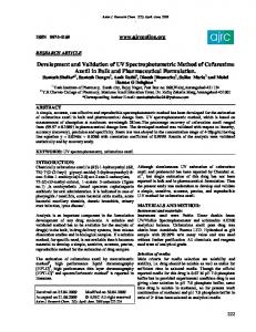
1. Axial flow For the axial flow case, the data set with 5m/s wind speed and -3 degrees pitch angle have been used. This results in a tip speed ratio of 7.5 where the angles of attack are below stall. Fig. 18 shows the comparisons with experiments in terms of normal force per unit of length. Apart from the results at the tip of the blade, where AWSM over predicts the normal force, the agreement with the experimental data is very good. However, it should be known that a standard BEM code over-predicts the tip forces to an even larger extent, as noted in [9]. This larger over-prediction from a BEM code was attributed to the fact that such code relies on the Prandtl tip loss factor, which has been derived using a very simplified wake model where AWSM models the flow near the tip in a much more physical way

Fig. 4 Normal force along the blade. Numerical-experimental comparison. 2. Yawed flow For the analysis in yawed conditions, experiments with 30 degrees yaw misalignment have been considered as test case; the wind speed is 5m/s and the pitch angle is -3 degrees. The azimuth distribution of normal force is computed at several radial locations (Fig. 5, at 0 degrees azimuth the blade is pointing upward). For all the positions, the shape of the curve is well taken; for some locations, the numerical predictions are vertically shifted. This difference with the experiments has to be taken into account in case of static-related calculations because the absolute value is important; however, for fatigue and yaw moment calculations, the differences between azimuth locations are important and not the single values.

Fig. 5 Normal force computed at different radial positions. Numerical-experimental comparison. Most interesting is to asses the phase in n(φr). In both measurements and calculations this phase is found to be different from root to tip, where the maximum force at the root occurs at φr ~ 270 degrees and at the tip it is shifted to φr ~ 90. The physical phenomena associated with this phase shift are described in [10] where it is explained to be a result of the variation of induced velocities over the azimuth angle. Near the tip this variation is mainly induced by tip vortices where it is induced by root vorticity at the more inboard positions, leading to an opposite phase. The variation in n(φr) can be assessed by considering its contribution to the yawing moment according to Fig. 6. Also in this case the agreement is very good. with negative yawing moments (i.e. destabilizing yawing moments) near the root and positive stabilizing yawing moments near the tip It is noted that most BEM methods model the variation in induced velocities with methods which were originally developed for helicopters in which the variation in velocities induced by tip vortices are included only. As such they model the maximum normal force at the root to be near φr ~ 90 degrees which leads to a positive yawing moment opposite to the results from this study.

Fig. 6 Yaw moment at different blade positions. Numerical-experimental comparison. B. MEXICO experiments Within the framework of the EU FP5 project MEXICO, a sophisticated aerodynamic experiment was designed, and executed in the Large Scale Low Speed Facility (LLF) of the German Dutch Wind tunnel Organization (DNW). The principal objective of this project was to significantly reduce these uncertainties by providing an experimental database, measured in a large wind tunnel under controlled and hence known conditions and by using the increased physical insight resulting from the experiments in engineering design methods. A three bladed rotor model of 4.5 m diameter was designed and manufactured, including a speed controller and pitch actuator. The blades were twisted and tapered. The airfoil were the DU91-W2-250 airfoil at the root, the RISO-A1-21 airfoil at the mid-span and the NACA643418 airfoil at the outer part. The model was instrumented with 148 Kulite® pressure sensors, distributed over 5 sections of the blades; strain gauges bridges were applied to the three blade roots for the registration of bending moments in two directions. The model was mounted on the wind tunnel 6 components balance, where total forces and moments were measured. Finally a large number PIV studies were programmed, to determine the flow field around the rotor, the inflow and near wake, and to track tip vortices. The experiment was designed for the 9.5*9.5 m2 open test section of the LLF. Detailed studies were executed to enable tunnel corrections on the measurements. 1. Yawed flow For the yawed flow condition, the data for 15m/s wind speed with a yaw angle of 30 and 45 degrees and a pitch angle of -2.3 degrees have been used. For non-yawed conditions a tunnel speed of 15 m/s and a pitch angle of -2.3 degrees reflects the design conditions where the angle of attack and the axial induction are expected to be optimal. In Fig. 7 and , the azimuth distribution of normal force is shown at several radial locations (at 0 degrees azimuth the blade is pointing upward). For all the positions, the shape of the curve is well taken; for some locations, the

numerical predictions are vertically shifted. As mentioned for NASA Ames experiments, this difference can affect static-related analyses, but not fatigue investigations and yaw moment calculations.

Fig. 7 Normal force computed at different radial positions. Numerical-experimental comparison, 30degrees yaw misalignment.

Fig. 8 Normal force computed at different radial positions. Numerical-experimental comparison, 45degrees yaw misalignment. Starting from these results, the yaw moment along the blade was calculated and compared with the experiments (Fig. 9).

Fig. 9 Yaw moment at different blade positions. Numerical-experimental comparison, 30degrees (on the left) and 45 degrees (on the right) yaw misalignments. 2. External field measurements Part of the MEXICO measurements was dedicated to determine the three-dimensional flow field around the wind turbine in detailed quantitative way. To do this, PIV technique was used and both the upstream and downstream regions of the turbine were explored; in particular, measurements were carried out in the form of an axial traverse at two radial stations and in the form of two radial traverse plans, one placed 0.3m upstream and one 0.3m downstream the rotor plan. By using AWSM, the induced velocity can be calculated in points of the external domain, so comparisons with experimental data coming from PIV measurements have been performed. For these tests, three values of wind speed have been used and all three components of velocity computed for axial traverse and radial traverse measurements (Fig. 10-Fig. 17). The u component denotes the axial component, v and w components denote the in-plan horizontal and vertical components.

Upstream radial traverse

Fig. 10 Numerical-experimental comparison; upstream radial traverse, u component (axial component) at 10, 15 and 24 m/s wind speed.

Fig. 11 Numerical-experimental comparison; upstream radial traverse, v component (in-plan horizontal component) at 10, 15 and 24 m/s wind speed.

Fig. 12 Numerical-experimental comparison; upstream radial traverse, w component (in-plan vertical component) at 10, 15 and 24 m/s wind speed.

Downstream radial traverse

Fig. 13 Numerical-experimental comparison; downstream radial traverse, u component (axial component) at 10, 15 and 24 m/s wind speed.

Fig. 14 Numerical-experimental comparison; downstream radial traverse, v component (in-plan horizontal component) at 10, 15 and 24 m/s wind speed.

Fig. 15 Numerical-experimental comparison; downstream radial traverse, w component (in-plan vertical component) at 10, 15 and 24 m/s wind speed.

Axial traverse

Fig. 16 Numerical-experimental comparison; axial traverse at 1.4m radial position, u (axial) component at 10, 15 and 24 m/s wind speed.

Fig. 17 Numerical-experimental comparison; axial traverse at 1.8m radial position, u (axial) component at 10, 15 and 24 m/s wind speed.

IV.

Non conventional configurations

One of the interesting features in AWSM code, is the possibility to model very general shaped geometries. Winglets and aft-swept blades are typical examples of non conventional shapes for wind turbine applications. Mostly due to commercial interests, no experimental data focused on these two features are available in literature. In the present research, results from preliminary numerical investigations are described, showing that AWSM predictions are consistent with physical expectations. A. Winglets Winglets are used to increase the blade efficiency and reduce the noise by decreasing the intensity of the tip vortices. A rectangular wing with 10m span and 1m chord is considered in this case as reference. Then, 0.3m high vertical winglets are added on the suction side and, at the same time, the wing span is shortened of the same amount

(Fig. 18) in order to keep constant the total wing surface. Because of this, the span of the wing with winglets is 6% shorter.

Fig. 18 Comparison between original rectangular wing and winglet-equipped. In Fig. 19, the comparison in terms of Cl along the span is shown. In accordance with the physic expectations, the effect is an increase in lift coefficient, and thus load, at the tip.

Fig. 19 Span-wise lift coefficient distribution. Comparison between geometry with and without winglets, AWSM predictions. B. Aft-swept blades Due to the increase in size of wind turbines, it is crucial to avoid excessive loads along the blade in order to prevent structural problems, especially the ones connected with fatigue. Aft-swept blades represent an innovative solution to reduce loads, loads fluctuations and, at the same time, noise. AWSM has been extended in order to take into account the deformation of the blade due to the torsion and the out of plane bending moments. A simplified model [13] has been adopted, in which the deformability of the geometry is concentrated at the root of the blade.

The Reference Wind Turbine (RWT) defined in the European project “Upwind” [14] has been used as baseline. Fig. 20 shows the comparison between the original straight geometry and the curved one. To investigate the effects of the curved geometry, the extreme gust condition defined in the IEC 61400 standards [15] has been analyzed. Fig. 21 shows the comparison in terms of time evolution of local angle of attack at the 92% of the blade. One effect due to the curved configuration is the general reduction in local angle of attack and loads; the second effect is related with the gust and with the fact that, during gust, the local angle of attack is oscillating. The oscillation for the aftswept blade is less than for the straight blade, showing that a reduction in fatigue loads is possible by adopting such solution.

Fig. 20 Comparison between the baseline RWT Upwind project blade and the modified aft-swept blade.

Fig. 21 Local angle of attack time evolution at the 92% of the blade. Comparison between the baseline RWT Upwind project blade and the modified aft-swept blade.

V.

Discussion of results

Looking at the comparisons, it should be noted that both for NASA Ames and MEXICO experiments the general agreement is really good. For yawed conditions, AWSM is able to produce very good predictions for the normal force and the yaw moment. This result is even more valuable if the main hypothesis of lifting line theory is recalled; the extension of the geometry in chord direction is negligible compared with the one in spanwise direction, so the real geometry is represented with a single line only. Spanwise and chordwise directions are defined by referring to the direction of the free-stream velocity; this means that for large values of yaw angle, the mathematical formulation should not be suitable for yawed flows, but, at least up to 45 degrees, AWSM results are quite accurate Part of the validation was focused on flow field measurements around the rotor. For different values of the wind speed, AWSM predictions are really close to the experiments for all the velocity components. Also in this context, the fact that the analysis is performed by considering a line and not the real geometry, like for panel methods or full Navier-Stokes codes, makes the results more valuable. For the non conventional configurations, the preliminary results are promising and in line with physical expectations, but more analyses and wind tunnel tests are necessary in order to fully validate AWSM predictions for these configurations. However, for these configurations, AWSM can be used in design or optimization context, where the ability to predict the correct trends are important, even more than the calculation of the absolute values.

VI.

Conclusions

A new code has been developed at ECN, based on generalized Prandtl’s lifting line and free vortex wake theory. Because of the new mathematical formulation, a very flexible tool has been obtained, able to predict the flow around a single or multiple components three-dimensional very general-shape geometries. Analyses on the blade are possible, as well as in the external field; yaw, pitch misalignments ground and non uniform wind conditions can be modelled. An intensive validation campaign has been performed by using experimental data coming from the NASA Ames and the MEXICO project experiments. Both axial and yawed flow conditions have been considered and in all the cases, the agreement between numerical predictions and experimental data was very good. From the MEXICO project, also PIV data concerning the velocity in the external field have been used, showing a very good agreement.

Finally, non-conventional configurations including winglets and aft-swept blades have been analyzed. More analyses and a validation using measurements on such configurations are necessary, but the preliminary results are promising and consistent with the expectations.

Acknowledgments Francesco Grasso would like to thank Teresa Maggio, from the University of Napoli “Federico II”, for the precious work done to include geometrical deformations in the AWSM code.

References [1]. Glauert, H., “Aerodynamic Theory”, Dover Publications Inc., 1935, Vol. 4, Division L, pp. 169-360. [2]. Hansen, M.O.L., ”Aerodynamics of Wind Turbines”, James & James, 2000, ISBN 1-902916-06-9. [3]. Van Garrel, A., “Development of a Wind Turbine Aerodynamics Simulation Module”, ECN, ECN-C-03-079, Petten, the Netherlands, August 2003. [4]. Grasso, F., “AWSM External Field Calculations”, ECN, ECN-X-09-043, Petten, the Netherlands, April 2009. [5]. Grasso, F., “AWSM Ground and Wind Shear Effects in Aerodynamic Calculations”, ECN, ECN-E-10-016, Petten, the Netherlands, February 2010. [6]. http://wind.nrel.gov/amestest/ [7]. Schepers, J.G., van Rooij, R.P.O.J.M., “Analysis of aerodynamic measurements on a model wind turbine placed in the NASA-Ames tunnel - ECN’s and TUD’s contribution to IEA Wind Task XX”, ECN, ECN-E-08-052, Petten, the Netherlands, October 2008. [8]. Schepers, J.G., “IEA Annex XX: Comparison between calculations and measurements on a wind turbine in yaw in the NASA-Ames wind tunnel”, ECN, ECN-E-07-072, Petten, the Netherlands, October 2007. [9]. Schepers, J.G., “IEA Annex XX: Comparison between calculations and measurements on a wind turbine in the NASA-Ames wind tunnel”, ECN, ECN-E-07-066, Petten, the Netherlands, December 2007. [10]. Schepers, J.G., “An engineering model for yawed conditions developed on basis of wind tunnel measurements”, AIAA/ASME Wind Energy Symposium, Reno USA, January 1999 [11]. Schepers, J.G., Snel, H., “Model Experiments in Controlled Conditions – Final Report”, ECN, ECN-E-07-042, Petten, the Netherlands, June 2007. [12]. Schepers, J.G., “EU projects in German Dutch Wind Tunnel, DNW”, IEA Symposium on the aerodynamics of wind turbines, NREL, USA, 4-5 December 2000.

[13]. Maggio, T., Grasso, F., Coiro, D.P., “Numerical Study on Performance of Innovative Wind Turbine Blade for Loads and Noise Reduction”, EWEA, EWEC 2011, Brussels, 14-17 March 2011. (accepted for publication) [14]. www.upwind.eu [15]. International Standard, “ Wind Turbine Generator Systems – Part1: Safety Requirements”, IEC, IEC 61400-1, 1999.