DEVELOPMENT OF PAVEMENT STRUCTURAL ANALYSIS DUE TO HORIZONTAL SURFACE FORCE BASED ON ELASTIC THEORY
Kunihito Matsui Professor of Civil Engineering Dept. of Civil and Environmental Engineering, Tokyo Denki University Hatoyama-Cho, Hiki-Gun, Saitama 350-0394, JAPAN
[email protected]
James W. Maina Chief Research Engineer Research Institute, Nippon Hodo Co., Ltd. 32-34, 3-Chome, Higashi-Shinagawa, Shinagawa-Ku, Tokyo 140-0002, JAPAN
[email protected] Quinxi Dong Transportation Technical Researcher, Airport Research Division Ministry of Land, Infrastructure and Transport 3-1-1, Nagase, Yokosuka, Kanagawa, 239-0826 JAPAN
[email protected] Takemi Inoue Director General Research Institute, Nippon Hodo Co., Ltd. 32-34, 3-Chome, Higashi-Shinagawa, Shinagawa-Ku, Tokyo 140-0002, JAPAN
[email protected]
PRESENTED FOR THE 2002 FEDERAL AVIATION ADMINISTRATION AIRPORT TECHNOLOGY TRANSFER CONFERENCE
05/02
Matsui et al.
1
ABSTRACT: In this research, a pavement is modeled as a multi-layered elastic system composed of a subgrade, which is assumed to be a semi-infinite medium on top which there are layers of finite thickness extended infinitely in a horizontal direction. A horizontal uniformly distributed load is assumed to act on the pavement surface. Expressing the displacement function of Navier’s equation in cylindrical coordinate system using harmonic and bi-harmonic functions, the analytical solution method is obtained through Hankel transformation and Hankel inverse transformation. In this research a computer program called Analysis of Multi-layered Elastic Systems (AMES), which can find pavement response due to multiple shear loadings, was developed. The accuracy of this program is confirmed by comparing results for a number of worked examples with results obtained using BISAR program. The comparison shows that the stress outputs from BISAR yield erroneous results at the pavement surface. Keywords: Multi-layered elastic systems, Navier's equation, harmonic function, bi-harmonic function, Hankel transformation, AMES
1. INTRODUCTION The Boussinesq solution, in case of concentrated vertical load acting on the surface of a semiinfinite body and also the Cerrutti solution in case of the action by concentrated horizontal load are well known. By integrating solutions of the concentrated load in the range of a circle, solutions for the case of circular uniformly distributed load can be obtained. However, it has not been possible to expand these solutions to a multi-layered structure. There are already numerous researches on the analytical solution based on the elastic theory. Most of these researches were performed before the invention of computers or when computer performance was still low and as a result most of the solutions were presented in the form of tables or graphs. Moreover, solutions presented were mostly based on a semi-infinite half space while the most famous solutions for a multilayer system were the Burmister’s solution for the case of axi-symmetric load and Kimura’s solution (1) that was intended for a two-layer system under a horizontal load. Most of these researches are well discussed by Poulos & Davis (2) and Kimura (3). Miyamoto (4) explains in details the analytical solution for horizontal circular load acting on a semi-infinite medium. BISTRO computer program may be the first program for analysis of a multilayer elastic system to be developed specifically for computer application. This program was developed in 1967 by the SHELL research group and was capable of performing axi-symmetric elastic analysis of a multilayered structure. One of the shortcomings of BISTRO was its inability to consider interface slip condition. Furthermore, since this program was intended for axi-symmetric analysis, it was not capable of performing asymmetric analysis of the multilayered structure. Due to these shortcomings, further modification was done on BISTRO and in 1973 BISAR program was developed. This program is capable of computing the solution (displacement, stress, strain, etc) for a given point in a multilayered elastic structure and is well trusted and highly evaluated among pavement engineers. Through development of AAMES (Axi-symmetric Analysis of Multi-layered Elastic Systems) (5), where effects of uniformly distributed vertical load were investigated, authors of this paper were able to check the accuracy and performance of BISAR program. Moreover, due
Matsui et al.
2
to limitations on the use of BISAR program together with a number of accuracy problems for the case of horizontal loading, it is hard to assert that enough check has been done on this program. The objective of this research was, therefore, to develop a computer program for analyzing the effect of horizontal load acting on the surface of a multilayered elastic system. By expressing Navier’s displacement equations in cylindrical coordinate system, Michell and Boussinesq displacement functions can be converted to harmonic and bi-harmonic functions. Theoretical solutions would be obtained by the application of Hankel transformation and Hankel inverse transformation. This procedure is fundamentally similar to BISAR program. However, the difference between this method and BISAR is the use of Hankel transformation. In BISAR program only Bessel functions of the first kind of zero and first orders were used while in this research Bessel functions of the first kind of zero, first and second orders are used. Furthermore, a propagation matrix was developed in the Hankel transformation range. By applying boundary and interface conditions in this range and determining constants of integration, Hankel inverse transformation could be performed. This solution, which was also used in the development of AAMES, is relatively simple. Evaluation of multiple loading cases is facilitated by placing measurement points as well as applied loads inside a global coordinate system. A local coordinate axis is introduced at the center of each loading point and subsequently, solutions for every measurement points are obtained. Since elastic theory is used, principle of superposition is also applied. Solutions for each case are then translated into the global coordinate system where overall superposition of the solutions is performed. Accuracy of this program is evaluated by comparing its results with the results obtained using BISAR. By way of this comparison, problems related to BISAR solutions when a horizontal load acts on the surface of a pavement structure are highlighted. The program developed in this research is called AMES (Analysis of Multi-layered Elastic Systems). At present, this program is set to consider a maximum of 100 loads, 100 layers and 10,000 measurement points.
2. PROBLEM DEVELOPMENT Pavement structure considered in this research is as shown in Figure 1(a). The subgrade is assumed to be a semi-infinite elastic medium on top of which there are horizontal layers of finite thickness extended infinitely in the horizontal direction. Each layer is made up of elastic, isotropic and homogeneous materials and the boundary condition is assumed to be rough. The circular load is assumed to act horizontally at the surface of the pavement as shown in Figure 1(b). Coordinate system used (X, Y, Z) is a global coordinate system, while coordinate system (x, y, z) is a local coordinate system. The origin of local coordinate system is at the center of the loading point and the direction of the x-axis is similar to the direction of the load. Furthermore, by introducing a cylindrical coordinate axis with common z-axis, the equilibrium equation can be expressed using Navier’s equations as follows:
∇ 2u +
1 ∂ ∂u u 1 ∂v ∂w u 2 ∂v + =0 − 2 − 2 + + 1 − 2ν ∂r ∂r r r ∂θ ∂z r r ∂θ
(1a)
Matsui et al.
3
thickness Young's modulus Poisson's ratio h1
E1
?1
h2
E2
?2
(0,0,0)
X 2a
loading point α
h i− 1
Ei − 1
? i− 1
hi
Ei
?i
θ
r measurement point
y
En
x
?n
Y
(a) Multilayer structural model
(b) Surface loading model Figure 1. Analytical model
∇ 2v +
1 1 ∂ ∂u u 1 ∂v ∂w v 2 ∂u + =0 + + − 2 − 2 1 − 2ν r ∂θ ∂r r r ∂θ ∂z r r ∂θ
(1b)
∇ 2w +
1 ∂ ∂u u 1 ∂v ∂w + + + = 0 1 − 2ν ∂z ∂r r r ∂θ ∂z
(1c)
where, ν is Poisson’s ratio and u , v, w are displacement components in r , ? , z directions of the cylindrical coordinate system. Since a horizontal uniformly distributed circular load acts on the pavement surface, the surface boundary conditions for r ≤a may be given as: τrz = − q cos θ τθz = q sin θ σz = 0
(2a)
where, τrz , τθz , σz are components of stress and q is a distributed load. Furthermore, for the case of r > a , the surface boundary conditions may be given as: τrz = τθz = σz = 0
(2b)
3. Method of Analysis 3.1. Hankel transformation of displacement and stress components Michell function, Φ , and Boussinesq function, Ψ , can be used to represent displacement components in Equations (1a, b, c) as:
u=−
∂2 Φ 2 ∂Ψ + ∂r∂z r ∂θ
(3a)
Matsui et al.
v=−
1 ∂2 Φ ∂Ψ − 2 r ∂θ∂z ∂r
w = 2(1 − ν)∇ 2 Φ −
∂2 Φ ∂z 2
4
(3b)
(3c)
where ∇ 2 is a Laplace operator in a cylindrical coordinate system:
∇2 =
∂2 1 ∂ 1 ∂2 ∂2 + + + ∂r 2 r ∂r r 2 ∂θ2 ∂z 2
(3d)
Using Φ and Ψ , stress components in a cylindrical coordinate system may be represented as: σr ∂ 2 ∂2 ∂ 1 1 ∂ Φ − 2 = ν∇ − − Ψ 2 2µ ∂z ∂θ r 2 r ∂r ∂r
(3e)
σθ ∂ 2 1 ∂ 1 ∂2 ∂ 1 1 ∂ = ν∇ − − 2 2 Φ+ 2 2 − Ψ ∂θ r 2µ ∂z r ∂r r ∂θ r ∂r
(3f)
σz ∂ ∂2 2 Φ (2 − ν)∇ − = 2 2µ ∂z z ∂
(3g)
τθz 1 ∂ ∂2 ∂2 2 = ( 1 ) − ν ∇ − Φ − Ψ 2µ r ∂θ ∂r∂z ∂z 2
(3h)
1 ∂2 τ zr ∂ ∂2 2 ( 1 ) = − ν ∇ − Φ + r ∂θ∂z Ψ 2µ ∂r ∂z 2
(3i)
1 ∂2 τrθ 1 ∂2 1 ∂ ∂2 1 ∂ = − − Φ + r 2 ∂θ2 ∂r 2 + r ∂r Ψ 2µ r ∂z∂θ r ∂r
(3j)
where µ is a shear modulus. Substituting Equations (3a, b) into Equations (1a, b, c) and rearrange yields:
∇ 4Φ = 0
(4a)
∇ 2Ψ = 0
(4b)
From the above relation, it is clear that a unique solution can be obtained if Φ and Ψ satisfy the equilibrium and compatibility equations. Fourier transformation of Φ and Ψ with respect to θ gives: ∞
Φ (r , θ, z ) = ∑ φm (r , z ) cos mθ m= 0
(5a)
Matsui et al.
Ψ (r , θ, z ) =
∞
∑ψ
m =0
m
(r , z ) sin mθ
5
(5b)
As shown in Figure (1b), since a uniformly distributed load is considered and by making reference to Equation (2a), only m = 1 may be used. This implies, letter m in the right hand side of Equations (5a, b) may be replaced by 1 to become: φ(r , z ) cos θ and ψ (r , z ) sin θ , respectively. Hankel transformation of φ(r , z ) , ψ (r , z ) would give: ∞
∫ rφ(r , z ) J (ξ r )dr = G(ξ, z )
(6a)
1
0
∞
∫ rψ (r, z ) J (ξ r )dr = H (ξ, z)
(6b)
1
0
Substituting Equations (5a, b) and (6a, b) into Equations (4a, b), yields: ∞
∫ 0
∞
∫ 0
2
d2 2 r∇ φJ 1 (ξ r )dr = dz 2 − ξ G (ξ, z ) = 0
(7a)
d2 2 r∇ 2 ψ J 1 (ξ r )dr = − ξ 2 dz H (ξ, z ) = 0
(7b)
4
And, solutions to these equations would be: G (ξ, z ) = ( A + Bz )e ξz + (C + Dz )e − ξz
(8a)
H (ξ, z ) = Ee ξz + Fe − ξz
(8b)
By substituting Equations (5a, b) and Equations (8a, 8b) into Equations (3a, b, and c) and performing Hankel transformation the following relation is obtained:
v ∞ u ∫0 r cos θ + sin θ J 2 (ξ r )dr ∞ u v r − J 0 (ξ r )dr A ∫0 cos θ sin θ B ∞ w ∫ r J 1 (ξ r )dr 0 C cos θ [ ] P = 1 ∞ σ D r z J 1 (ξ r )dr ∫ 0 E cos θ ∞ τθz τ zr + J 2 (ξ r ) dr F ∫0 r sin θ cos θ ∞ τθz τ zr ∫0 r sin θ − cos θ J 0 (ξ r )dr
(9)
where, [ P1 ] is 6 ×6 matrix whose components are shown in Table 1. Coefficients A, B, C , D, E, F are constants of integration determined by the use of boundary and interface conditions. Values of
Matsui et al. Table 1. [ P1 ]matrix
(
2 ξz ξ e 2 ξz − ξ e 2 ξz
− ξ e
3 ξz − 2µξ e
) ξz ξz ξ(1 + ξz )e
−
− ξ( − 2 + ξz + 4 ν) e
(
2 − ξz − ξ e
ξ1 + ξz e
2 − ξz ξ e ξz
− 2µξ( − 1 + ξz + 2ν)e
ξz
) − ξz − ξz ξ(1 − ξz )e
ξ1 − ξz e −
2 − ξz ξ e
− ξ( 2 + ξz − 4 ν) e
− ξz
2ξe 2ξe
ξz ξz
2 ξe 2 ξe
− ξz − ξz
0
0 0
3 − ξz 2µξ e
− ξz 2 2µξ (1 + ξz − 2 ν) e
0
3 ξz 2µξ e
ξz 2 2µξ (ξz + 2ν) e
3 − ξz 2µξ e
− ξz 2 2µξ ( ξz − 2ν) e
2 ξz 2µξ e
3 ξz 2µξ e
ξz 2 2µξ (ξz + 2ν) e
3 − ξz 2µξ e
− ξz 2 2µξ ( ξz − 2ν) e
2 ξz − 2µξ e
2 − ξz − 2 µξ e
2 − ξz 2µξ e
Table 2. [ P2 ]matrix 3 ξz 2 µξ e
ξz 2 2 µξ (1 + ξz + 2ν ) e
3 − ξz − 2µξ e
− ξz 2 2µξ (1 − ξz + 2 ν) e
0
0
3 ξz 2µξ e
ξz 2 2 µξ (1 + ξz + 4ν ) e
3 − ξz − 2µξ e
− ξz 2 2µξ (1 − ξz + 4 ν) e
0
0
0
0
0
0
2 ξz 2µξ e
2 − ξz 2µξ e
σr , σθ , τrθ given by Equation (10) would be computed after A, B, C , D, E, F have been determined: A ∞ σr 2µ u 2µ v B r J r dr + + ( ξ ) 1 ∫0 r r cos θ cos θ sin θ ∞ σ σ r C θ P2 ] =[ ∫0 r cos θ + cos θ J 1 (ξ r )dr D ∞ τ 2µ u 2µ v E rθ ∫0 r sin θ + r cos θ + r sin θ J 1 (ξ r )dr F
(10)
P2 ]is 3 ×6 matrix whose components are shown in Table 2. where, [ Hankel inverse transformation in a cylindrical coordinate system could be performed on the Hankel transform of displacement and stress components to give: ∞ u u v v + = ∫ ξ + J 2 (ξ r )d ξ 0 cos θ sin θ cos θ sin θ
u v − = cos θ sin θ
∞
u
∫ ξcos θ − 0
∞ w w = ∫ ξ J 1 (ξ r ) d ξ 0 cos θ cos θ
v J 0 (ξ r )d ξ sin θ
(11a)
(11b)
(11c)
6
Matsui et al. ∞ σ σz = ∫ ξ z J 1 (ξ r )d ξ 0 cos θ cos θ
(11d)
τθz τ zr + = sin θ cos θ
∫ ξsin θ +
τθz τ zr − = sin θ cos θ
∫ ξsin θ −
∞
τθz
τzr J 2 (ξ r ) d ξ cos θ
(11e)
τθz
τzr J 0 (ξ r ) d ξ cos θ
(11f)
0
∞
0
∞ σ σr 1 u 1 v 1 u 1 v + + = ∫ ξ r + + J 1 (ξ r )d ξ 0 cos θ r cos θ r sin θ cos θ r cos θ r sin θ
(11g)
σr σθ + = cos θ cos θ
(11h)
∞
σr
∫ ξcos θ + 0
σθ J 1 (ξ r )dξ cos θ
∞ τ τ rθ 1 u 1 v 1 u 1 v + + = ∫ ξ rθ + + J 1 (ξ r )d ξ 0 sin θ r cos θ r sin θ θ θ sin r cos r sin θ
7
(11i)
where the top bar represents Hankel transformation of the corresponding displacement and stress components. 3.2. Expansion to multilayered pavement structure Figure 1(a) was considered in this analysis. With reference to Equation (9), displacement and stress components for the i th layer would be given as follows:
u (i ) ( z , ξ) v (i ) ( z , ξ) cos θ + sin θ (i) (i ) u ( z , ξ) − v ( z , ξ) Ai (ξ) cos θ sin θ B (ξ) w (i ) ( z , ξ) i C (ξ) cos θ =[ P1 ( z , ξ)] i (i ) σz ( z , ξ) Di (ξ) Ei (ξ) cos θ τθ(iz) ( z , ξ) τrz(i ) ( z , ξ) + Fi (ξ) θ cos θ (sin (i ) i) τθz ( z , ξ) − τrz ( z , ξ) cos θ sin θ
(12)
For the case where displacement and stress components at the boundary between i th and (i + 1) th layers are assumed to be continuous and local coordinate systems, whose origins are at the surface of each layer, are introduced the following relations would be obtained:
Matsui et al. u (i ) (hi , ξ) v (i ) (hi , ξ) u (i + 1) (0, ξ) v (i + 1) (0, ξ) + + θ θ θ cos sin θ cos sin (i + 1) (i) (i ) ( i + 1) (0, ξ) v (0, ξ) u (hi , ξ) − v (hi , ξ) u − cos θ sin θ sin θ cos θ w (i + 1) (0, ξ) w (i ) (hi , ξ) θ cos cos θ = ( i + 1) (i) σz (0, ξ) σz (hi , ξ) cos θ cos θ τθ(iz) (hi , ξ) τrz(i ) (hi , ξ) τθ(iz+ 1) (0, ξ) τrz(i + 1) (0, ξ) + + cos θ θ cos θ sin θ (isin ( i + 1) ( i + 1) ) (i) τθz (hi , ξ) − τrz (hi , ξ) τθz (0, ξ) − τrz (0, ξ) cos θ sin θ cos θ sin θ
8
(13)
By using Equations (12) and (13) it is possible to develop propagation matrix showing the relationship between stress and strain components of the 1st layer and constants of integration of the lowest layer (the N th layer). Furthermore, when the value of z approaches infinity in case of the N th layer (semi-infinite medium), stress and strain components approach zero and constants of integration will become: An = Bn = E n = 0 . Hankel transformation of the uniformly distributed circular load, q , whose radius is a and acts on the surface of the pavement would be given as: τθ(1z) (0, ξ) τrz(1) (0, ξ) + sin θ cos θ = 0 (1) (1) τθz (0, ξ) − τrz (0, ξ) q (ξ) cos θ sin θ
(14)
q (ξ) = ∫r (2q )J 0 (ξ r )dr =
(15)
where, a
0
2qa J 1 (ξ a) ξ
By taking into consideration boundary and interface conditions and representing propagation matrix components by t ij , the relationship between the 1st and N th layers would be: u (1) (0, ξ) v (1) (0, ξ) + θ sin θ t11 (cos 1) (1) u (0, ξ) − v (0, ξ) t 21 cos θ sin θ t 31 w (1) (0, ξ) = t 41 cos θ t 51 0 0 t 61 q (ξ)
t 21
t 31
t 41
t 51
t 22
t 32
t 42
t 52
t 23
t 33
t 43
t 53
t 24
t 34
t 44
t 54
t 25 t 26
t 35 t 36
t 45 t 46
t 55 t 56
t 61 0 t 62 0 t 63 C n t 64 D n t 65 0 t 66 Fn
and constants of integration for the N th layer would be determined by:
(16)
Matsui et al.
C n Dn = F n
t 34 t 35 t 36
t 44 t 45 t 46
−1
t 64 t 65 t 66
0 0 q (ξ)
9
(17)
By using Equation (17), together with Equations (12) and (13), constants of integration ( Ai (ξ) , Bi (ξ) , C i (ξ) , Di (ξ) , Ei (ξ) , and Fi (ξ) ) for all the layers could be computed in a stepwise process. This means values on the right hand side of Equations (9) and (10) would be obtained, and by applying Hankel inverse transformation it is possible to compute values on the left hand side of Equations (11a) - (11i) to obtain strain and stress components. However, when r = 0 , computation of σr and τrθ using Equations (11g) and (11i) is not straightforward because of the term 1 r . The L’Hopital rule is used to solve these equations. The accuracy of computation of Equations (11a) - (11i) is highly influenced by the accuracy of the semi-infinite integration. In this study, a relatively accurate double exponential (DE) integration method (6, 7) was used, as in the AAMES program, to solve semi-infinite integration.
4. ANALYSIS FOR MULTIPLE LOADINGS Figure 2 shows the loading point and measurement point as represented in a global coordinate system ( X , Y , Z ) . For multiple loadings acting on the pavement surface, the transformation S from cylindrical to global coordinate system is represented by: matrix [] cos(α + θ) sin( α + θ) 0 [S ]= − sin( α + θ) cos(α + θ) 0 0 0 1
(18)
By using this transformation matrix, displacement components in global coordinate system would be represented as:
(0,0,0)
X 2a
loading point (X, Y, 0) α θ
x
r
y
measurement point
Y
( X + r cos(θ + α ) , Y + r sin(θ + α ) , 0)
Z
z
Figure 2. Global and local coordinate axes
Matsui et al. 10
2a = 30 cm
Q = 49 kN
θ = 30°
ν1 = 0.35 E1 = 2500 MPa
y
x h1 = 10 cm
ν2 = 0.35
E2 = 280 MPa ν3 = 0.4
E3 = 50 MPa
h2 = 35 cm
h3 = ∞
z Figure 3. Load and layer properties in example 1
0.01
0.015
0.02
0.025
0.003 0
10
10
20
20
depth (cm)
depth (cm)
0.005 0
30 40 50 60
0.007
0.009
0.011
0.013
30 40 50 60
(a) u r (cm)
-0.4 -0.3 -0.2 -0.1
0
0.1
0.2 0.3
0.4
0
0
10
10
20 30 40
(b) u ? (cm)
-0.7 -0.6 -0.5 -0.4 -0.3 -0.2 -0.1
depth (cm)
depth (cm)
0.005
20 30 40
50
50
60
60 (c) t ?z (MPa)
(d) t rz (MPa) GAMES
BISAR
Figure 4. Comparison of AMES and BISAR results (example 1)
0
0.1
Matsui et al. 11 u U T V = [S ] v w W
(19)
whereas, stress components in local coordinate system would be represented as:
σx τxy τ xz
τ xy σz τ yz
τxz σr T τ yz = [S ] τrθ σz τrz
τr θ
τrz τθz [S ] σz
σθ τθz
(20)
Displacement and stress components for all individual loading will be obtained in this manner. Finally, by using the principal of superposition, the overall displacement and stress components in the global coordinate system due to all the loadings will be obtained by superimposing results from the individual loadings.
5. NUMERICAL COMPUTATIONS 5.1. Example 1 AMES and BISAR programs were used to obtain pavement response due to horizontal load acting on the surface of a three-layer pavement structure as shown on Figure 3. Figure 4 shows pavement response at the point of loading ( r = 0 cm ), when the depth z was varied between 0 and 60cm. Figures 4(a) and 4(b) indicate a good agreement between results of pavement displacements obtained using AMES and BISAR programs. Results for shearing stress are presented in Figures 4(c) and 4(d). Results for shearing stress, τθz , are shown in Figure 4(c). The difference between the two programs is more evident near the surface as the difference between the results start increasing and at the surface where there is a sudden change of value for the case of BISAR result. This sudden change of shear stress value at the surface of the pavement is not natural and appears 2a = 30 cm
Q = 49 kN
θ = − 30°
ν1 = 0.35 E1 = 2500 MPa
y
θ = 30° ν2 = 0.35
ν3 = 0.4
E2 = 280 MPa E3 = 50 MPa
x h1 = 10 cm
h2 = 35 cm
h3 = ∞
z Figure 5. Load and layer properties in example 2
Matsui et al. 12 to lack the support of basic engineering judgment. Results for shear stress, τrz , show similar trend although there is no sudden change of BISAR result at the surface. This difference can mainly be attributed to the difference in the level of accuracy in the respective programs when solving semiinfinite Hankel transformations presented in Equation (9).
0.02
0.03
0.04
-0.006 0
10
10
20
depth (cm)
depth (cm)
0.01 0
30 40 50
-0.002
-0.001
0.2
0.25
20 30 40
-0.2
0
u x (cm) 0.2
(b) 0.4
0.6
0.8
0 0
10
10
20
20
depth (cm)
0
30 40 50
0.05
u z (cm)
0.1
0.15
30 40 50 60
(c) s x (MPa)
(d) s z (MPa)
-0.6
-0.4
-0.2
0
0.2
0.4
0 10 depth (cm)
depth (cm)
-0.003
60 (a)
60
-0.004
50
60
-0.4
-0.005
20 30 40 50 60
(e) t xz (MPa) GAMES
BISAR
Figure 6. Comparison of AMES and BISAR results (example 2)
Matsui et al. 13 5.2. Example 2 AMES and BISAR programs were again used to obtain pavement response due to two horizontal loads acting on the surface of a three-layer pavement structure as shown on Figure 5. Figure 5 shows the loading condition in the global coordinate system. Figures 6(a-e) show variations of displacement and stress components on a 0 to 60cm depth along the z-axis. Displacement results shown in Figures 6(a) and 6(b) indicate a good agreement between the two programs. However, similar to example 1 above, stress results presented in Figures 6(c, d, e) indicate differences between these two programs especially for measurement points at and near the surface. The difference between these two programs starts increasing near the surface and there is a sudden jump for the case of BISAR results at the surface of the pavement structure. 6. CONCLUSIONS In this study, development of analytical solutions for pavement response due to uniformly distributed horizontal circular force acting on the surface of a multilayer pavement structure were presented. Accuracy of the program developed was evaluated by comparison of its results with BISAR results. The following conclusions were drawn from the results obtained: • The accuracy of the theoretical solution developed in this study was confirmed by comparison of AMES results with BISAR results • Figure 4(c) in example 1 and Figures 6(c, d, e) in example 2 show a discontinuous pattern of shearing stress obtained using BISAR. This is an indication of computational errors at or near the multilayer structure for the part of BISAR. • Examples 1 and 2 confirm that AMES program can be used to analyze multilayer structural response due to a single or multiple horizontal loadings with relatively good accuracy. AKNOWLEDGMENT This research study was partly sponsored by Program for Promoting Fundamental Transport (Project No. 2000-03). The authors would like to acknowledge the support of every one involved in this project, especially Mr. Ozawa, who is a former student at Tokyo Denki University. REFERENCES 1) Kimura, T. Pavement stress due to horizontal load, JSCE, No. 133, pp. 21-28, 1966. 2) Poulos, H. G. and Davis, E. H. Elastic Solutions for Soil and Rock Mechanics, John Wiley & Sons, 1974. 3) Kimura, T. Soil stress, Kashima Publication, 1978. 4) Miyamoto, H. Theory of Three-Dimensional Elastic Analysis (in Japanese), 1977. 5) Matsui, K., Maina, J.W., Inoue, T. Axi-symmetric Analysis of Elastic Multilayer System Considering Interface Slips. 2nd International symposium on maintenance and rehabilitation of pavements and technological control, Alabama, USA, 2001, CD-ROM. 6) Ooura, T. and Mori, M.: The Double Exponential Formula for Oscillatory Functions over Half Infinity Integral, Journal of Computational and Applied Mathematics 38, pp.353-360. 1991. 7) Mori, M.: Fortran77 Programming for Numerical Computations (revised edition), Iwanami Shoten. 2000.4